Abstract
In Systems Biology, the complex relationships between different entities in the cells are modeled and analyzed using networks. Towards this aim, a rich variety of gene regulatory network (GRN) inference algorithms has been developed in recent years. However, most algorithms rely solely on gene expression data to reconstruct the network. Due to possible expression profile similarity, predictions can contain connections between biologically unrelated genes. Therefore, previously known biological information should also be considered by computational methods to obtain more consistent results, such as experimentally validated interactions between transcription factors and target genes. In this work, we propose XGBoost for gene regulatory networks (XGRN), a supervised algorithm, which combines gene expression data with previously known interactions for GRN inference. The key idea of our method is to train a regression model for each known interaction of the network and then utilize this model to predict new interactions. The regression is performed by XGBoost, a state-of-the-art algorithm using an ensemble of decision trees. In detail, XGRN learns a regression model based on gene expression of the two interactors and then provides predictions using as input the gene expression of other candidate interactors. Application on benchmark datasets and a real large single-cell RNA-Seq experiment resulted in high performance compared to other unsupervised and supervised methods, demonstrating the ability of XGRN to provide reliable predictions.
1. Introduction
A main direction in the Systems Biology field is detecting and studying the complex relationships between different molecules in the cell. For this, network modeling has been extensively used to analyze the interactions between genes, mRNAs, proteins or metabolites [1], as well as other entities, such as diseases [2,3] or drugs [4,5]. This approach has generated the Network Medicine field, where complex diseases are analyzed, which can concurrently affect many genes [6,7,8]. To study cell mechanisms, an abundance of large-scale gene expression experiments were conducted using microarray or RNA sequencing (RNA-Seq) techniques, and data are available via publicly accessible databases. The gene regulatory network (GRN) inference problem refers to reconstructing a network consisting of interactions between transcription factors (TFs) and their target genes. TFs are proteins that bind to DNA and regulate the expression of the genes, i.e., they can activate or inhibit the transcription.
Substantial research interest has attracted the de novo GRN inference, namely, to construct a network based only on gene expression data. Towards this, a plethora of algorithms has been developed utilizing various mathematical and computational methods in the last two decades. Initial efforts focused on finding expression similarities via correlation (e.g., WGCNA [9]) or mutual information (MI) (e.g., ARACNE [10], CLR [11]) and more recently, other variations of them, such as sparse correlation [12], conditional MI [13,14] and partial information decomposition [15]. Several studies tried to model the gene transcription process using linear [16,17] or non-linear [18,19] ordinary differential equations or stochastic differential equations [20]. Other approaches used Boolean networks [21], statistical/probabilistic methods, for instance, Gaussian graphical models [22], Bayesian networks [23,24,25,26], and regression analysis (such as linear regression [27], Lasso regression [28,29], least angles regression [30]). Another category is relying on machine learning methods, for example, support vector machines (SVM) (e.g., SIRENE [31]), random forest (e.g., GENIE3 [32], Jump3 [33]), XGBoost [34,35] and neural networks [36]. Finally, methods for more specific problems have been developed, such as a method using deep neural networks on microscopy images recording spatial gene expression [37] or a method to jointly learn GRNs in different species using orthology and Bayesian inference [38]. Several reviews are available on the topic [39,40,41,42], showing that each method makes different assumptions and takes advantage of different biological characteristics. Thus it can be most effective on specific data or problems. In [42], an extensive comparison was performed, and it was concluded that the performance is highly variable on different data, confirming the “no free lunch theorem”.
Moreover, the GRN reconstruction algorithms can be categorized based on two interesting characteristics, locality and supervision [41]. Regarding locality, algorithms can be characterized as global if the same approach is applied on all genes and as local if specific characteristics of each node are taken into account. An example of locality improving network inference results is the pair of unsupervised algorithms ARACNE [10] and CLR [11]. In ARACNE, first, pair-wise MI is calculated, and then a network pruning step follows to eliminate indirect connections, while in CLR, an adaptive background correction step is performed before pruning to keep interactions that are important for both connected nodes. Another widely used local GRN algorithm is GENIE3 [32], which handles each gene separately. Specifically, for each target gene, considering all other genes as candidate regulators (or a subset of genes if a list of TFs is given), a random forest is trained using the target’s expression as output and regulators’ expression as input, and subsequently, the variable importance measure of the trained model is used to evaluate the rank of the potential regulators for the target gene.
Supervision refers to the inclusion of prior knowledge to improve modeling. Hence algorithms can be divided into supervised and unsupervised. Considering that human gene expression data contain measurements of about 20,000 genes, usually in few hundreds of samples, this consists of a “large p small n” problem. Thus inferring a biologically meaningful GRN relying solely on gene expression data is an extremely hard computational task. Therefore, supervised methods have emerged, which can provide more accurate results since embedding a priori knowledge in the form of experimentally validated interactions can lead to the exclusion of spurious interactions between biologically unrelated genes, despite possible expression profile similarity [43]. Examples include [44], where functional associations were used as priors to solve an optimization problem, and [45], which used network motifs to learn probabilistic graphical models. Of great interest is the machine-learning category because, by their nature, these methods are based on supervised learning algorithms. A characteristic example is the SVM-based method SIRENE [31], which solves a classification problem separately for each TF to determine if a gene is its target a or not. The operation of SIRENE requires as input a list of known TFs and their targets as positive examples, while due to the absence of negative examples, a cross-validation scheme is used on the unknown genes, considering a data subset as non-interacting examples. Finally, classification is performed using the expression of the unknown genes to predict their category (targets or non-targets).
Focusing on ensemble tree methods, i.e., random forest and XGBoost, they have been successfully applied in a wide range of Systems Biology problems, but in most cases, in an unsupervised mode. In detail, random forest models have been trained in order to obtain variable importance measurements and select the most discriminative variables; for instance, to rank single-nucleotide polymorphisms (SNPs) [46] or microRNAs [47] according to the relationship with a disease, to detect differentially expressed pathways between two conditions [48] and for GRN in GENIE3 method [32] as previously described. Similarly, XGBoost has been used to classify subpathways and select the most discriminative ones with variable importance [49]. For GRN, in GRNBoost2 [34], the same approach with GENIE3 is followed simply by replacing random forest with XGBoost, while in BiXGBoost [35], the same concept is used in two directions to select both the best regulators and targets for each gene. However, from a machine learning perspective, there are two distinct phases, model training on some labeled data and prediction on new unlabeled data. In the aforementioned applications, models are trained to obtain the variable importance measurement, but they are not used for prediction. Therefore, the machine-learning algorithms are not exploited to their full potential. A notable exception where the trained regression random forest model is utilized is predicting new gene targets of microRNAs [50].
Since in GRN inference, we are interested in prediction, this motivated us to create an appropriate training and testing approach to benefit from the generalization abilities of machine-learning methods. In this study, we present a local supervised method named XGBoost for gene regulatory networks (XGRN), aiming to model a biological network’s interactions and predict new similar interactions utilizing gene expression profiles. Specifically, each previously known interaction is represented with a regression XGBoost model built on the expression profiles of the two interactors. Using the trained model, we predict the gene expression of the second interactor with other genes as input, and then we compare the prediction with the actual values to infer if similar patterns are obtained. Thus these other genes could be possible interactors. In the case of GRN reconstruction, based on some known TF-target gene interactions, our method predicts other possible target genes of the TFs. The proposed method was applied on benchmark microarray data and a real single-cell RNA-Seq (scRNA-Seq) dataset with very high performance compared to other methods.
2. Materials and Methods
2.1. Extreme Gradient Boosting (XGBoost)
Extreme gradient boosting (XGBoost) [51] is a novel classifier based on an ensemble of classification and regression trees, which are optimized using gradient boosting. Boosting is an ensemble learning algorithm that trains a (weak) model and then sequentially trains an enhanced model, which attempts to improve the errors made by the predictor in the previous iteration. To achieve this, the new model in each iteration is built to fit the residuals of the previous model. In the gradient boosting technique, the gradients of the optimization function are used with a learning rate [52].
Let the output of a tree be
where x is the input vector and is the value of the corresponding leaf q. The output of the ensemble of K trees is
Of note, the output is the summary of the output of all models, instead of the more common mean used, e.g., in random forest.
The XGBoost algorithm defines the following objective function J for minimization:
where t is the step, the first summary is over the train loss function L (such as mean squared error—MSE) between real class and output for the N samples, and the second summary is the regularization term, which controls the complexity of the model and helps to avoid overfitting.
In XGBoost, the complexity in the second term of Equation (3) is defined as:
where T is the number of leaves, γ is a dataset-specific pseudo-regularization hyperparameter, and λ is the L2 norm for leaf weights.
The loss function L can be approximated with Taylor expansion using second-order gradients. For a leaf node i, let and be the first and second-order gradients of the loss function, respectively. Then, the optimal weights can be found for this tree:
where is the set of leaf nodes. Finally, the optimal value of the objective function is:
The value of the objective function is used as a score to evaluate the current tree structure and thus is used to select the best split at each step.
2.2. GRN Reconstruction
Briefly, in XGRN, given an expression dataset and a set of known interactions, we model each interaction between two genes with a regression XGBoost model. Thus, this model can learn from the respective expression profiles the function governing this pair of regulator and target. Then, this trained model can be tested on expression values from a different gene to examine if its behavior could be explained by the model learned for this regulator. The workflow of the proposed method is summarized in Figure 1.
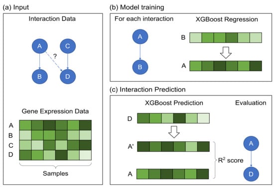
Figure 1.
The workflow of the XGRN method. (a) The input consists of known interactions and a gene expression dataset. Next, using the directed A–B interaction, we predict a score for the A–D interaction. (b) An XGBoost regression model is trained for each known interaction using the corresponding expression profiles. As input is set, the target’s expression and as output the regulator’s expression. (c) Using the trained model with the expression of gene D as input, a score is provided for interaction A–D based on R2 measurement comparing the predicted gene expression A’ and the actual gene expression A.
In detail, for each interaction, in the form of “gene A interacts with gene B”, we train an XGBoost regressor using gene’s B expression profile as input and A’s expression profile as output variable. Then, this trained model is used on other gene profiles to determine if they could be potential interactors with gene A. Specifically, the expression profile of each other gene is set as input, and a prediction of A’s profile is obtained as output. Finally, the prediction and the actual profile are compared using some metrics, such as mean squared error (MSE), mean absolute error (MAE) or R2. A low error indicates that the samples in testing show similar patterns as in training. Intuitively, we attempt to learn the function “B is regulated by A”, thus as A, we will use profiles of TFs and as B the target genes. Since a TF usually has more than one known target, we train several models (one for each interaction), and hence we obtain multiple prediction values for a candidate target. We combine them by keeping the minimum error (for MSE or MAE) or the maximum value for R2 as the final prediction score.
XGRN was implemented in Python 3.8.3 and is available at https://github.com/geodimitrak/XGBoost-GRN (accessed on 19 April 2021).
2.3. Data
The DREAM project organizes annual challenges in Systems Biology, with tasks such as GRN reconstruction, providing benchmark expression datasets along with the true structure of the network for evaluation, i.e., a list of interacting gene pairs. The proposed method was evaluated on the datasets of the DREAM 4 “In Silico Network Challenge” [53] (five small networks) and DREAM 5 “Network Inference Challenge” [54] (four networks of different sizes). The data consist of preprocessed gene expression profiles and a list indicating which genes are possible TFs. From DREAM 4, the steady-state data were used.
Next, a scRNA-Seq dataset was downloaded from the NCBI Gene Expression Omnibus database with accession number GSE86469 [55]. This study performed a scRNA-Seq experiment with 638 islet cells from pancreas tissue, including 20,565 genes obtained from non-diabetic (ND) and type 2 diabetes (T2D) human organ donors. The authors detected significant differences between ND and T2D human islet samples, providing useful insights into islet biology and diabetes pathogenesis. As the gold standard, a list of 6289 interactions between 280 TFs and 2287 target genes in a human was used obtained from [56]. We limited our analysis only to the genes common in the gold standard and the gene expression dataset. A logarithmic transformation was applied to data before analysis. Additionally, during training and testing, we discarded samples with 0 values as dropouts. A summary of the data details is provided in Table 1.

Table 1.
Dataset information.
2.4. Evaluation
To assess the accuracy of our method, the area under receiver operator curve (AUROC) was used, which is computed as the area under receiver operator curve (ROC), which in turn is the plot of the true-positive rate versus the false-positive rate at various values of threshold. This way, there is no need to select a specific threshold to characterize a predicted interaction as true or not since AUROC calculates a summary result taking into account all possible thresholds.
3. Results
To better demonstrate the operation of XGRN, in Figure 2, we present an example of gene expression profiles from D52. In Figure 2a, a regression model was trained using the profiles of a TF and a known gene target to learn the relationship between them. Then it was tested using the profile of another gene, which was an actual target of the same TF, and the output was very similar to TF’s profile based on the R2 metric. Thus this interaction was predicted as true. In Figure 2b, the same procedure was repeated, but in testing, the gene was not a target of this TF. In this case, the output of regression had a low R2 value. Thus this potential interaction was correctly considered false.
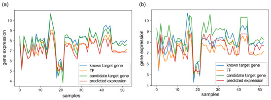
Figure 2.
(a) An XGBoost regression model is trained based on a known TF-target gene interaction using the expression profile of the target gene as input (blue) and the TF’s profile as output (orange). Then, the model was used in testing with input the profile of a second candidate gene (green), which was a target of this TF. The prediction (red) matched the profile of the TF (R2 = 0.81); thus, this gene was considered as a target. (b) Similarly, the same model was tested on another candidate gene (green), which was not the target of this TF. The prediction (red) presented low similarity with TF (orange) (R2 = 0.23); thus, this candidate interaction was considered false.
3.1. Parameter Selection
To test the robustness of results concerning parameter selection and to optimize performance, before applying XGRN on large real datasets, we tried it on the small DREAM 4 datasets with varying values of parameters. We ranged the number of estimators (number of trees) trained in the model from 10 to 100 and the learning rate (LR) from 0.01 to 0.5. The results are shown in Figure 3a for the average of the five datasets. Regarding the number of trees, with higher values, the performance was improved, as expected. Additionally, with a higher learning rate, the results were improved. However, for LR ≥ 0.05, the performance remained stable regardless of the number of trees. Therefore, to balance performance and execution time, in subsequent results, we selected LR = 0.1 and 50 trees. The ROC curves for these settings are shown in Figure 3b. The maximum depth parameter was also examined but had a small effect on performance. For the selected values of LR = 0.1 and 50 trees, trying depth from 4 to 10, the results ranged from 0.79 to 0.81. Therefore, we set the maximum depth to 5 for the following results (also in previous results in Figure 2, it was set to 5). A higher depth, except the larger execution time, may lead the model to overfit and subsequently to provide inferior predictions in testing. Thus we did not choose a larger value, despite the slightly higher accuracy in the small datasets of DREAM 4. Other XGBoost parameters were left to default values (γ = 0, λ = 1).
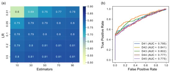
Figure 3.
(a) Performance in terms of AUROC of XGBoost when varying the number of estimators (trees) and the learning rate (LR) parameters. The results are the average of the five DREAM 4 datasets. (b) ROC curves of DREAM 4 datasets using XGBoost with LR = 0.05 and 50 trees.
Finally, we compared the results using R2, mean squared error (MSE) and mean absolute error (MAE) as the output of our method when comparing the predicted with the actual expression (Table 2). R2 led to superior results, although the difference was small. This can be explained by the fact that R2 has an upper limit of 1, making easier comparisons among different models, while the magnitude of the other two metrics is affected by the expression levels.
Table 2.
Performance (AUROC) of regression evaluation methods.
3.2. GRN Inference Performance
To obtain a set of interactions for training, we randomly selected a percentage of the ground truth interactions. We present the performance of XGRN based on 50% of known interactions provided as input, while the effect of the supervision percentage is discussed later. Finally, to compare our results, the supervised method SIRENE was used, as well as the best performing unsupervised method per dataset among the participants in the DREAM challenges [54], which are GENIE3 for D51, Pearson’s correlation coefficient for D52, two-way ANOVA for D53 and a correlation-based meta-predictor for D54. Using the same approach as with our method, SIRENE was given as input 50% of the ground truth interactions. The other parameters of SIRENE were left to default values (SVM with radial basis function (RBF) and cost parameter C = 1000). The performance of XGRN surpassed SIRENE and other unsupervised methods in all datasets (Figure 4). The difference of AUROC with unsupervised methods was very large in D51 (10%), D52 (19%), D54 (10%) and slightly better in D53 (2%). Remarkably, SIRENE performed worse than unsupervised methods in D52 and D53, almost the same in D51, and only in D54, it displayed higher performance, equal to our method.
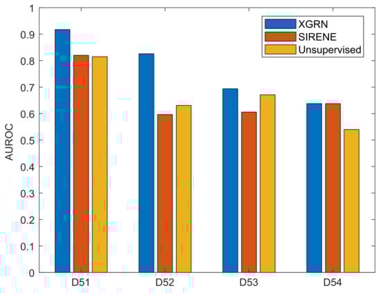
Figure 4.
Performance of XGRN, SIRENE and unsupervised methods on DREAM 5 datasets. The best unsupervised method was GENIE3 for D51, Pearson’s correlation coefficient for D52, two-way ANOVA for D53 and a correlation-based meta-predictor for D54.
In the real scRNA-Seq dataset, the performance of XGRN was 72.3% using 10% supervision, increased to 80.9% with 30% supervision and reached 84.5% with 50% supervision. This shows that the proposed method is effective not only in microarray gene expression but in RNA-Seq data as well, which are nowadays the standard methodology to measure gene expression.
3.3. Effect of Prior Knowledge Percentage
Finally, we tested the effect on performance when using different percentages of prior knowledge. Results are shown for the D51 dataset, which displayed the highest performance between the benchmark datasets, but other datasets showed similar trends. As can be observed in Figure 5, the performance increased as the prior knowledge increased. This is expected since with more known data, more models are trained for each TF, and there are higher chances to find other genes exhibiting similar patterns with known targets. Most importantly, XGRN resulted in high performance even with a small percentage of prior knowledge. Specifically, with only 10% of the known interactions available, the AUROC was about 82%, which was close to the maximum obtained by SIRENE or other unsupervised methods. This shows that our method can be applied and predict interactions effectively even if a small fraction of the real network has been discovered.
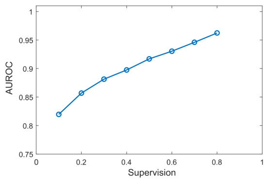
Figure 5.
Performance of XGRN concerning supervision percentage in D51.
4. Discussion
In this study, we presented XGRN, a local supervised method with the aim to model known interactions of a gene network and to predict new similar interactions. Specifically, exploiting gene expression data in combination with some known TF-target gene interactions, other candidate target genes of each TF are predicted. We repeat that this is performed by training an XGBoost regression model on TF and target gene expressions and applying the trained models on other genes’ profiles to infer if these candidate target genes result in similar patterns with the known target. In contrast to most unsupervised de novo GRN reconstruction methods, where each gene-gene combination is examined resulting in a matrix (where N is the number of the genes), here previously validated biological interactions are used, enabling us to focus only on TFs for model training, which are a small percentage of the genes. It is important that our method is local and focuses on each TF separately since it has been shown that GRN is sparse [57] and scale-free [58], namely some TFs have many targets, while most of them have few specific targets. Therefore, we can adapt to each TF’s characteristics. The independent modeling of each interaction is a key characteristic for users, who would like to focus only on a specific interaction subset, for example, a TF of interest or a specific pathway.
Regarding supervision, it was confirmed the statement that supervised methods could help to increase performance [43]. Especially in D54, which is the largest dataset, the best unsupervised method provided an AUROC of 54%, which is not useful as a prediction since it is marginally higher than the chance level of 50%. Furthermore, it has been shown that several older GRN methods do not perform well in scRNA-Seq data [59]. Hence it is important to test a method not only on benchmark DREAM datasets but also on real RNA-Seq experimental data.
The core concept of XGRN resembles the supervised learning performed by SIRENE for GRN inference, where a binary classification problem is solved separately for each TF to predict if a gene is its target or not, based on expression profiles of known targets [31]. The operation of SIRENE requires as input a set of TFs and their targets as positive examples, while in the absence of negative examples, a cross-validation scheme is used on the unknown genes. It is noted that in this approach, the regulator profile is not utilized. An advantage of using regression instead of classification as in SIRENE is that we can utilize both the target and the regulator expression profiles. Moreover, this scheme can overcome the absence of negative examples, avoiding the hypothesis that the absence of interaction in a dataset can be interpreted as a negative training example.
Interestingly, our method is a generic framework that can be implemented using any regression method. However, XGBoost is a very recent, high-performing method, which builds a complex regression model, able to capture various non-linear functions. We note that gene expression experiments can contain inherent noise, therefore, we would like to avoid overfitting a model [60]. Ensemble tree algorithms, such as random forest and XGBoost, help towards building a more generalized model by selecting as parameters many trees and a small maximum depth for each tree. In addition, machine-learning algorithms, such as the tree-based, are purely data-driven and model-free. Namely, no assumptions are made about the distribution of the variables or the relationships between them (which is the case in regression methods based on a specific mathematical model [27,28,29,30]). Moreover, tree-based regression is not affected by the absolute expression level (high or low). Finally, there are few parameters to be fine-tuned, but they have a small effect on the quality of results. Thus there is no need for an exhaustive search for optimal values, which in addition may lead to overfitting to training data.
Noteworthy, the directionality of the interaction is taken into account by our method, which is a desired characteristic in TF-target networks, as well as in other cases, such as cellular pathways. If we switch the input and output, then we would model the relationship “a gene is targeted by a TF” and would set as testing input the profiles of other TFs to detect if they target this gene. Results were similar in this reverse case. Thus for clarity, we presented here only the first direction. A limitation of our method is that we cannot predict new targets of TFs without any known gene targets. However, even if a small number of relationships between TFs and target genes are known, we showed that the proposed method could accurately recover the network structure. This is very important since we do not know if biological networks are close to their complete form or not, especially for less studied organisms.
In conclusion, XGRN can deliver reliable results from a biological point of view, providing output networks very similar to the ground truth. We confirmed that supervised methods combining both expression data with network structure could outperform unsupervised ones. The proposed approach to train regression models on known interacting node pairs provided accurate predictions, proving its efficiency. The high-performance was achieved by employing XGBoost for regression, a recent model-free method. In general, the development of accurate computational tools cannot only help biological data analysis but also can be used as a first step before designing an experiment to provide indicative results for later experimental validation, reducing the cost by trying only the most promising directions. Furthermore, we believe that a gene expression prediction approach can be extremely valuable to various different applications beyond network reconstruction. In the future, we plan to apply this method to other interaction data, such as protein–protein interactions (PPIs) or pathways. Algorithms integrating these different information types are very important for advanced comprehension of the cellular mechanisms. Finally, recent research focus has been shifted on network-based differential gene expression, such as pathways and subpathways [61,62,63,64]. Thus, we aim to adapt the proposed method for differential gene expression detection by using in testing the expression profile of the same gene in different conditions.
Funding
This research received no external funding.
Data Availability Statement
Code and data used in this work are publicly available at https://github.com/geodimitrak/XGBoost-GRN (accessed on 19 April 2021).
Conflicts of Interest
The authors declare no conflict of interest.
References
- Ideker, T.; Krogan, N.J. Differential network biology. Mol. Syst. Biol. 2012, 8. [Google Scholar] [CrossRef] [PubMed]
- Vidal, M.; Cusick, M.E.; Barabási, A.L. Interactome networks and human disease. Cell 2011, 144, 986–998. [Google Scholar] [CrossRef] [PubMed]
- Lee, D.S.; Park, J.; Kay, K.A.; Christakis, N.A.; Oltvai, Z.N.; Barabasi, A.-L. The implications of human metabolic network topology for disease comorbidity. Proc. Natl. Acad. Sci. USA 2008, 105, 9880–9885. [Google Scholar] [CrossRef] [PubMed]
- Csermely, P.; Korcsmáros, T.; Kiss, H.J.M.; London, G.; Nussinov, R. Structure and dynamics of molecular networks: A novel paradigm of drug discovery: A comprehensive review. Pharmacol. Ther. 2013, 138, 333–408. [Google Scholar] [CrossRef]
- Liu, Q.; Muglia, L.J.; Huang, L.F. Network as a biomarker: A novel network-based sparse bayesian machine for pathway-driven drug response prediction. Genes (Basel) 2019, 10, 602. [Google Scholar] [CrossRef]
- Network Medicine; Loscalzo, J., Barabási, A.-L., Silverman, E.K., Eds.; Harvard University Press: London, UK, 2017; ISBN 9780674545533. [Google Scholar] [CrossRef]
- Dimitrakopoulou, K.; Dimitrakopoulos, G.N.; Sgarbas, K.N.; Bezerianos, A. Tamoxifen integromics and personalized medicine: Dynamic modular transformations underpinning response to tamoxifen in breast cancer treatment. OMICS 2014, 18, 15–33. [Google Scholar] [CrossRef]
- Dimitrakopoulou, K.; Dimitrakopoulos, G.N.; Wilk, E.; Tsimpouris, C.; Sgarbas, K.N.; Schughart, K.; Bezerianos, A. Influenza a immunomics and public health omics: The dynamic pathway interplay in host response to H1N1 infection. Omi. A J. Integr. Biol. 2014, 18, 167–183. [Google Scholar] [CrossRef]
- Langfelder, P.; Horvath, S. WGCNA: An R package for weighted correlation network analysis. BMC Bioinform. 2008, 9, 559. [Google Scholar] [CrossRef]
- Margolin, A.A.; Nemenman, I.; Basso, K.; Wiggins, C.; Stolovitzky, G.; Favera, R.D.; Califano, A. ARACNE: An algorithm for the reconstruction of gene regulatory networks in a mammalian cellular context. BMC Bioinform. 2006, 7, S7. [Google Scholar] [CrossRef]
- Faith, J.J.; Hayete, B.; Thaden, J.T.; Mogno, I.; Wierzbowski, J.; Cottarel, G.; Kasif, S.; Collins, J.J.; Gardner, T.S. Large-scale mapping and validation of Escherichia coli transcriptional regulation from a compendium of expression profiles. PLoS Biol. 2007, 5, e8. [Google Scholar] [CrossRef]
- Serra, A.; Coretto, P.; Fratello, M.; Tagliaferri, R. Robust and sparse correlation matrix estimation for the analysis of high-dimensional genomics data. Bioinformatics 2018, 34, 625–634. [Google Scholar] [CrossRef]
- Zhang, X.; Zhao, J.; Hao, J.-K.; Zhao, X.-M.; Chen, L. Conditional mutual inclusive information enables accurate quantification of associations in gene regulatory networks. Nucleic Acids Res. 2015, 43, e31. [Google Scholar] [CrossRef]
- Zhao, J.; Zhou, Y.; Zhang, X.; Chen, L. Part mutual information for quantifying direct associations in networks. Proc. Natl. Acad. Sci. USA 2016, 113, 5130–5135. [Google Scholar] [CrossRef]
- Chan, T.E.; Stumpf, M.P.H.; Babtie, A.C. Gene Regulatory Network Inference from Single-Cell Data Using Multivariate Information Measures. Cell Syst. 2017, 5, 251–267. [Google Scholar] [CrossRef]
- Matsumoto, H.; Kiryu, H.; Furusawa, C.; Ko, M.S.H.; Ko, S.B.H.; Gouda, N.; Hayashi, T.; Nikaido, I. SCODE: An efficient regulatory network inference algorithm from single-cell RNA-Seq during differentiation. Bioinformatics 2017, 33, 2314–2321. [Google Scholar] [CrossRef]
- Frankowski, P.C.A.; Vert, J.P. Gene regulation inference from single-cell RNA-seq data with linear differential equations and velocity inference. Bioinformatics 2020, 36, 4774–4780. [Google Scholar] [CrossRef]
- Ma, B.; Fang, M.; Jiao, X. Inference of gene regulatory networks based on nonlinear ordinary differential equations. Bioinformatics 2020, 36, 4885–4893. [Google Scholar] [CrossRef]
- Herrera-Delgado, E.; Perez-Carrasco, R.; Briscoe, J.; Sollich, P. Memory functions reveal structural properties of gene regulatory networks. PLoS Comput. Biol. 2018, 14, e1006003. [Google Scholar] [CrossRef]
- Tian, T.; Burrage, K. Stochastic models for regulatory networks of the genetic toggle switch. Proc. Natl. Acad. Sci. USA 2006, 103, 8372–8377. [Google Scholar] [CrossRef]
- Barman, S.; Kwon, Y.-K. A Boolean network inference from time-series gene expression data using a genetic algorithm. Bioinformatics 2018, 34, i927–i933. [Google Scholar] [CrossRef]
- Zhang, R.; Ren, Z.; Chen, W. SILGGM: An extensive R package for efficient statistical inference in large-scale gene networks. PLoS Comput. Biol. 2018, 14, e1006369. [Google Scholar] [CrossRef] [PubMed]
- Friedman, N. Inferring Cellular Networks Using Probabilistic Graphical Models. Science 2004, 303, 799–805. [Google Scholar] [CrossRef] [PubMed]
- Dimitrakopoulou, K.; Tsimpouris, C.; Papadopoulos, G.; Pommerenke, C.; Wilk, E.; Sgarbas, K.N.; Schughart, K.; Bezerianos, A. Dynamic gene network reconstruction from gene expression data in mice after influenza A (H1N1) infection. J. Clin. Bioinforma. 2011, 1, 27. [Google Scholar] [CrossRef] [PubMed]
- Xing, L.; Guo, M.; Liu, X.; Wang, C.; Zhang, L. Gene Regulatory Networks Reconstruction Using the Flooding-Pruning Hill-Climbing Algorithm. Genes 2018, 9, 342. [Google Scholar] [CrossRef]
- Staunton, P.M.; Miranda-Casoluengo, A.A.; Loftus, B.J.; Gormley, I.C. BINDER: Computationally inferring a gene regulatory network for Mycobacterium abscessus. BMC Bioinform. 2019, 20, 466. [Google Scholar] [CrossRef]
- Magnusson, R.; Gustafsson, M. LiPLike: Towards gene regulatory network predictions of high certainty. Bioinformatics 2020, 36, 2522–2529. [Google Scholar] [CrossRef]
- Omranian, N.; Eloundou-Mbebi, J.M.O.; Mueller-Roeber, B.; Nikoloski, Z. Gene regulatory network inference using fused LASSO on multiple data sets. Sci. Rep. 2016, 6, 20533. [Google Scholar] [CrossRef]
- Ghosh Roy, G.; Geard, N.; Verspoor, K.; He, S. PoLoBag: Polynomial Lasso Bagging for signed gene regulatory network inference from expression data. Bioinformatics 2021, 36, 5187–5193. [Google Scholar] [CrossRef]
- Haury, A.C.; Mordelet, F.; Vera-Licona, P.; Vert, J.P. TIGRESS: Trustful Inference of Gene REgulation using Stability Selection. BMC Syst. Biol. 2012, 6, 145. [Google Scholar] [CrossRef]
- Mordelet, F.; Vert, J.P. SIRENE: Supervised inference of regulatory networks. Bioinformatics 2008, 24. [Google Scholar] [CrossRef]
- Huynh-Thu, V.A.; Irrthum, A.; Wehenkel, L.; Geurts, P. Inferring regulatory networks from expression data using tree-based methods. PLoS ONE 2010, 5, e12776. [Google Scholar] [CrossRef]
- Huynh-Thu, V.A.; Sanguinetti, G. Combining tree-based and dynamical systems for the inference of gene regulatory networks. Bioinformatics 2015, 31, 1614–1622. [Google Scholar] [CrossRef]
- Moerman, T.; Aibar Santos, S.; Bravo González-Blas, C.; Simm, J.; Moreau, Y.; Aerts, J.; Aerts, S. GRNBoost2 and Arboreto: Efficient and scalable inference of gene regulatory networks. Bioinformatics 2019, 35, 2159–2161. [Google Scholar] [CrossRef]
- Zheng, R.; Li, M.; Chen, X.; Wu, F.X.; Pan, Y.; Wang, J. BiXGBoost: A scalable, flexible boosting-based method for reconstructing gene regulatory networks. Bioinformatics 2019, 35, 1893–1900. [Google Scholar] [CrossRef]
- Maraziotis, I.A.; Dragomir, A.; Thanos, D. Gene regulatory networks modelling using a dynamic evolutionary hybrid. BMC Bioinformatics 2010, 11, 140. [Google Scholar] [CrossRef]
- Yang, Y.; Fang, Q.; Shen, H. Bin Predicting gene regulatory interactions based on spatial gene expression data and deep learning. PLoS Comput. Biol. 2019, 15, e1007324. [Google Scholar] [CrossRef]
- Penfold, C.A.; Millar, J.B.A.; Wild, D.L. Inferring orthologous gene regulatory networks using interspecies data fusion. Bioinformatics 2015, 31, i97–i105. [Google Scholar] [CrossRef][Green Version]
- Noor, A.; Serpedin, E.; Nounou, M.; Nounou, H.; Mohamed, N.; Chouchane, L. An overview of the statistical methods used for inferring gene regulatory networks and protein-protein interaction networks. Adv. Bioinform. 2013, 2013, 953814. [Google Scholar] [CrossRef]
- Lecca, P.; Priami, C. Biological network inference for drug discovery. Drug Discov. Today 2013, 18, 256–264. [Google Scholar] [CrossRef]
- Emmert-Streib, F.; Dehmer, M.; Haibe-Kains, B. Gene regulatory networks and their applications: Understanding biological and medical problems in terms of networks. Front. Cell Dev. Biol. 2014, 2, 38. [Google Scholar] [CrossRef]
- Muldoon, J.J.; Yu, J.S.; Fassia, M.K.; Bagheri, N. Network inference performance complexity: A consequence of topological, experimental and algorithmic determinants. Bioinformatics 2019, 35, 3421–3432. [Google Scholar] [CrossRef] [PubMed]
- Maetschke, S.R.; Madhamshettiwar, P.B.; Davis, M.J.; Ragan, M.A. Supervised, semi-supervised and unsupervised inference of gene regulatory networks. Brief. Bioinform. 2014, 15, 195–211. [Google Scholar] [CrossRef] [PubMed]
- Studham, M.E.; Tjärnberg, A.; Nordling, T.E.M.; Nelander, S.; Sonnhammer, E.L.L. Functional association networks as priors for gene regulatory network inference. Bioinformatics 2014, 30, i130–i138. [Google Scholar] [CrossRef] [PubMed]
- Siahpirani, A.F.; Roy, S. A prior-based integrative framework for functional transcriptional regulatory network inference. Nucleic Acids Res. 2017, 45, e21. [Google Scholar] [CrossRef]
- Wang, Y.; Goh, W.; Wong, L.; Montana, G. Random forests on Hadoop for genome-wide association studies of multivariate neuroimaging phenotypes. BMC Bioinform. 2013, 14 (Suppl. 1), S6. [Google Scholar] [CrossRef]
- Wuchty, S.; Arjona, D.; Li, A.; Kotliarov, Y.; Walling, J.; Ahn, S.; Zhang, A.; Maric, D.; Anolik, R.; Zenklusen, J.C.; et al. Prediction of associations between microRNAs and gene expression in glioma biology. PLoS ONE 2011, 6, e14681. [Google Scholar] [CrossRef]
- Dimitrakopoulos, G.N.; Balomenos, P.; Vrahatis, A.G.; Sgarbas, K.; Bezerianos, A. Identifying disease network perturbations through regression on gene expression and pathway topology analysis. In Proceedings of the 2016 38th Annual International Conference of the IEEE Engineering in Medicine and Biology Society (EMBC), Orlando, FL, USA, 16–20 August 2016; pp. 5969–5972. [Google Scholar] [CrossRef]
- Dimitrakopoulos, G.N.; Vrahatis, A.G.; Plagianakos, V.; Sgarbas, K. Pathway analysis using XGBoost classification in Biomedical Data. In Proceedings of the 10th Hellenic Conference on Artificial Intelligence (SETN ’18), Patras, Greece, 9–12 July 2018; ACM: New York, NY, USA, 2018; p. 46. [Google Scholar] [CrossRef]
- Dimitrakopoulos, G.N.; Dimitrakopoulou, K.; Maraziotis, I.A.; Sgarbas, K.; Bezerianos, A. Supervised method for construction of microRNA-mRNA networks: Application in cardiac tissue aging dataset. In Proceedings of the 2014 36th Annual International Conference of the IEEE Engineering in Medicine and Biology Society (EMBC), Chicago, IL, USA, 26–30 August 2014; pp. 318–321. [Google Scholar] [CrossRef]
- Chen, T.; Guestrin, C. XGBoost: A scalable tree boosting system. In Proceedings of the ACM SIGKDD International Conference on Knowledge Discovery and Data Mining, San Francisco, CA, USA, 13–17 August 2016; ACM: New York, NY, USA, 2016; pp. 785–794. [Google Scholar] [CrossRef]
- Friedman, J.H. Greedy function approximation: A gradient boosting machine. Ann. Stat. 2001, 29, 1189–1232. [Google Scholar] [CrossRef]
- Marbach, D.; Prill, R.J.; Schaffter, T.; Mattiussi, C.; Floreano, D.; Stolovitzky, G. Revealing strengths and weaknesses of methods for gene network inference. Proc. Natl. Acad. Sci. USA 2010, 107, 6286–6291. [Google Scholar] [CrossRef]
- Marbach, D.; Costello, J.C.; Küffner, R.; Vega, N.M.; Prill, R.J.; Camacho, D.M.; Allison, K.R.; Kellis, M.; Collins, J.J.; Aderhold, A.; et al. Wisdom of crowds for robust gene network inference. Nat. Methods 2012, 9, 796–804. [Google Scholar] [CrossRef]
- Lawlor, N.; George, J.; Bolisetty, M.; Kursawe, R.; Sun, L.; Sivakamasundari, V.; Kycia, I.; Robson, P.; Stitzel, M.L. Single-cell transcriptomes identify human islet cell signatures and reveal cell-type-specific expression changes in type 2 diabetes. Genome Res. 2017, 2, 208–222. [Google Scholar] [CrossRef]
- Madhamshettiwar, P.B.; Maetschke, S.R.; Davis, M.J.; Reverter, A.; Ragan, M.A. Gene regulatory network inference: Evaluation and application to ovarian cancer allows the prioritization of drug targets. Genome Med. 2012, 4, 41. [Google Scholar] [CrossRef]
- Espinosa-Soto, C. On the role of sparseness in the evolution of modularity in gene regulatory networks. PLoS Comput. Biol. 2018, 14, e1006172. [Google Scholar] [CrossRef]
- Ouma, W.Z.; Pogacar, K.; Grotewold, E. Topological and statistical analyses of gene regulatory networks reveal unifying yet quantitatively different emergent properties. PLoS Comput. Biol. 2018, 14, e1006098. [Google Scholar] [CrossRef]
- Chen, S.; Mar, J.C. Evaluating methods of inferring gene regulatory networks highlights their lack of performance for single cell gene expression data. BMC Bioinform. 2018, 19, 232. [Google Scholar] [CrossRef]
- Raser, J.M.; O’Shea, E.K. Noise in gene expression: Origins, consequences, and control. Science 2005, 309, 2010–2013. [Google Scholar] [CrossRef]
- Tarca, A.L.; Draghici, S.; Khatri, P.; Hassan, S.S.; Mittal, P.; Kim, J.S.; Kim, C.J.; Kusanovic, J.P.; Romero, R. A novel signaling pathway impact analysis. Bioinformatics 2009, 24, 75–82. [Google Scholar] [CrossRef]
- Vrahatis, A.G.; Balomenos, P.; Tsakalidis, A.K.; Bezerianos, A. DEsubs: An R package for flexible identification of differentially expressed subpathways using RNA-seq experiments. Bioinformatics 2016, 32, 3844–3846. [Google Scholar] [CrossRef]
- Judeh, T.; Johnson, C.; Kumar, A.; Zhu, D. TEAK: Topology Enrichment Analysis frameworK for detecting activated biological subpathways. Nucleic Acids Res. 2013, 41, 1425–1437. [Google Scholar] [CrossRef]
- Vrahatis, A.G.; Dimitrakopoulos, G.N.; Tsakalidis, A.K.; Bezerianos, A. Identifying miRNA-mediated signaling subpathways by integrating paired miRNA/mRNA expression data with pathway topology. In Proceedings of the 2015 37th Annual International Conference of the IEEE Engineering in Medicine and Biology Society (EMBC), Milan, Italy, 25–29 August 2015; pp. 3997–4000. [Google Scholar] [CrossRef]


Publisher’s Note: MDPI stays neutral with regard to jurisdictional claims in published maps and institutional affiliations. |
© 2021 by the author. Licensee MDPI, Basel, Switzerland. This article is an open access article distributed under the terms and conditions of the Creative Commons Attribution (CC BY) license (https://creativecommons.org/licenses/by/4.0/).