Modelling of Conditional Scalar Dissipation Rate in Turbulent Premixed Combustion

Abstract

In turbulent premixed flames, for the mixing at a molecular level of reactants and products on the flame surface, it is crucial to sustain the combustion. This mixing phenomenon is featured by the scalar dissipation rate, which may be broadly defined as the rate of micro-mixing at small scales. This term, which appears in many turbulent combustion methods, includes the Conditional Moment Closure (CMC) and the Probability Density Function (PDF), requires an accurate model. In this study, a mathematical closure for the conditional mean scalar dissipation rate, $<N_c|\zeta >$, in Reynolds, Averaged Navier–Stokes (RANS) context is proposed and tested against two different Direct Numerical Simulation (DNS) databases having different thermochemical and turbulence conditions. These databases consist of lean turbulent premixed V-flames of the CH4-air mixture and stoichiometric turbulent premixed flames of H2-air. The mathematical model has successfully predicted the peak and the typical profile of $<N_c|\zeta >$with the sample space ζ and its prediction was consistent with an earlier study.

1. Introduction

The turbulence and chemical reaction predominately influence the structure of turbulent premixed flames. The turbulence scales range from the Kolmogorov length scale, ${\eta }_k$, with a characteristics velocity, $u_k^{\prime }$, to the integral length scale, Λ, with characteristic velocity, $u^{\prime }.$ The combustion scales are typically represented by the laminar flame thickness, ${\delta }_L^0$, and the flame speed, $S_L^0$. 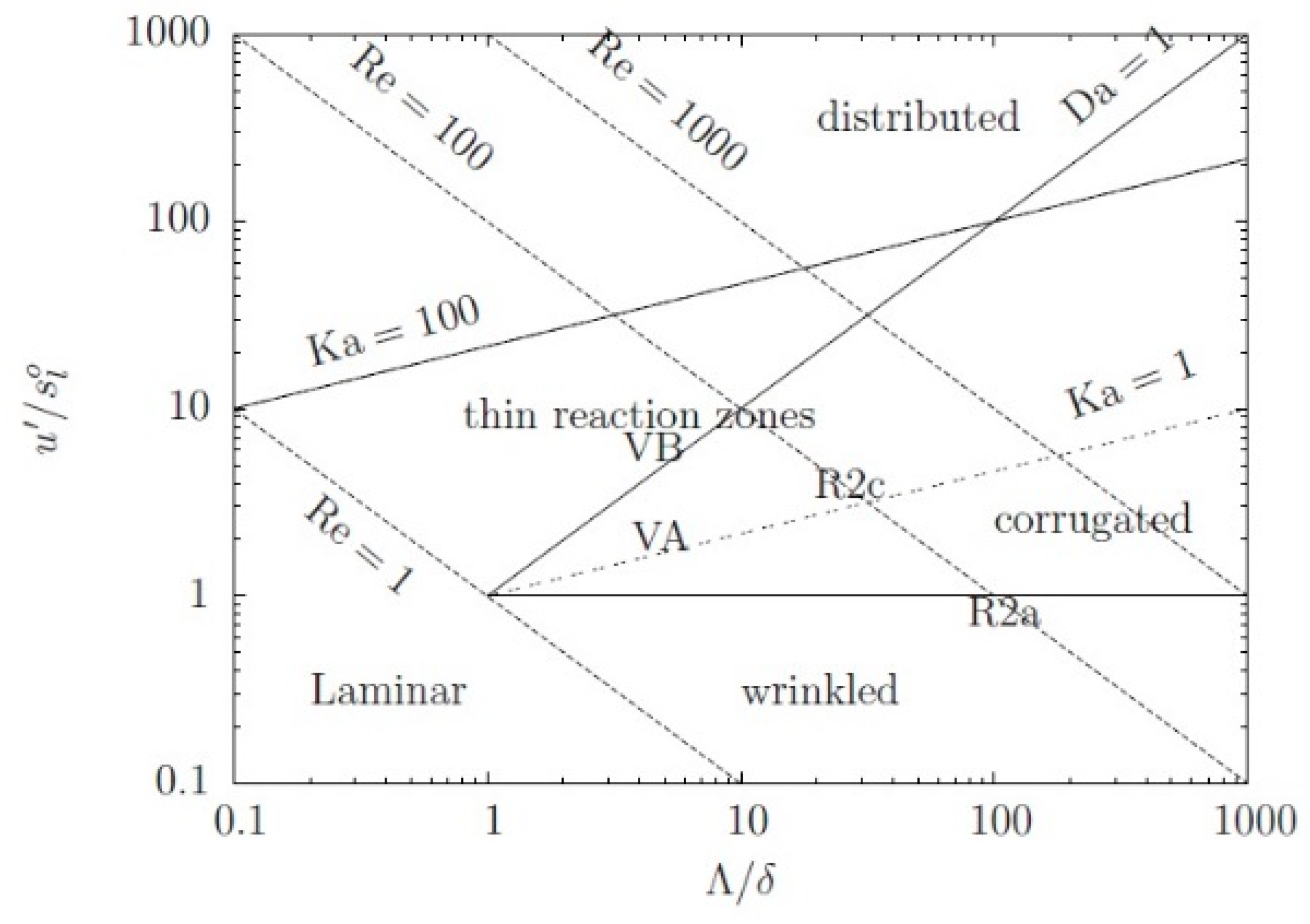These effects are widely classified on the regime diagram [1] by the ratios of turbulence intensity to laminar burning velocity,$u^{\prime }/S_L^0,$ and integral length scale to laminar flame thickness,$\mathsf{\Lambda }/{\delta }_L^0$. At low Karlovitz number, Ka, (defined as the ratio of the chemical time scale ${\tau }_c$ and the smallest turbulent time scale ${\tau }_k$) turbulence stretch the flame surface by folding the flame front. It should be noted that at high Ka number, the local flame structure also changes. Nevertheless, the extent of change has a positive correlation with the magnitude of Ka number [2].

In turbulent premixed flames, the scalar dissipation rate describes the local micro-mixing of the relevant scalar. It signifies the dissipation rate of progress variable variance, which is predominantly affected by the coupling between turbulence, diffusion and chemical reaction. This term appears in many turbulent combustion methods such as Flamelets [2], Probability Density Function (PDF) [3] and Conditional Moment Closure (CMC) [4,5] and requires a sensible closure. A substantial amount of experimental and modelling literature has been published on the scalar dissipation rate for non-premixed [6,7,8,9] and premixed [10,11,12,13,14] combustion. In premixed flames, a reasonable model for the scalar dissipation rate must account for the interaction between turbulence, chemical reaction and molecular diffusion; consequently, using turbulent time scale alone has proved to be insufficient [11,15]. Recent developments in the modelling of the mean dissipation rate for turbulent premixed flames are reviewed first in Section 2 before proceeding with the modelling of the conditional scalar dissipation rate.

The conditional scalar dissipation rate, $<N_c|\zeta >$, which appears in the CMC and PDF, is associated with the mean dissipation rate as follows

$$\widetilde{{ϵ}_c}={\int }_0^1<N_c|\zeta >\tilde{p}\left(\zeta \right)d\zeta ,$$

(1)

where $\zeta$ is the sample space for the progress variable, c and $\tilde{p}$ is the Favre average PDF. The progress variable, c, measures the reaction progress in premixed combustion. It is defined using the temperature, T or using the fuel mass fraction, $Y_f$, as [6]

$$c_T=\frac{T-T_u}{T_b-T_u},$$

(2)

where$T_u$and $T_b$, respectively, signify the temperature of the unburnt and burnt mixture in adiabatic laminar flames and

$$c_f=1-\frac{Y_f}{Y_f^u}.$$

(3)

$Y_f^u$denotes the fuel mass fraction in the unburnt side. For unity, Lewis numbers are defined as the ratio of the thermal diffusivity to mass diffusivity and for a single-step chemical reaction $c_f= c_T$ [16]. An alternative choice using sensible enthalpy is also possible [4].

The marginal PDF for c is $p\left(\zeta \right)$, which can be determined either by solving their transport equations or by presuming a PDF shape. In this work, the PDF profiles are obtained from [17,18,19] where $\tilde{c}$ and $\widetilde{c^{{″}^2}}$are obtained by solving their transport equations. To be noted that the Favre PDF, $\tilde{p}\left(\zeta \right)$, is related to $p\left(\zeta \right)$ [20] by

$$p\left(\zeta \right)= \frac{\overline{\rho }\tilde{p}\left(\zeta \right)}{\rho }=\frac{1+\tau \zeta }{1+\tau \tilde{c}}\tilde{p}\left(\zeta \right).$$

(4)

where τ is the heat release parameter and is defined as $\tau =\left(T_b-T_u\right)/T_u$(with the subscripts b and u, respectively, represent burnt and unburnt mixtures). ρ is the density.

The mean scalar dissipation, $\widetilde{{ϵ}_c}$, rate in Reynolds Averaged Navier Stokes (RANS) context is defined as

$$\overline{\rho }\widetilde{{ϵ}_c}=\overline{\rho {\mathcal{D}}_c\left(\frac{\partial c^{″}}{\partial x_i}\right)\left(\frac{\partial c^{″}}{\partial x_i}\right),}$$

(5)

where ${\mathcal{D}}_c,$the molecular diffusivity and c is the fluctuation of the progress variable. The over-bar represents Reynolds averaging, and the tilde indicates density, ρ, weighted averaging.

This study aims to obtain closure for the conditional scalar dissipation rate,$<N_c|\zeta >,$ and to test the model using two different Direct Numerical Simulation (DNS) databases [17,19]. It is worth mentioning that the second stage of this work is to implement the proposed model in the RANS-CMC method to compute turbulent premixed flames. The outcome was encouraging and will be published in a subsequent article.

The frame of this article is as follows. In Section 2, the proposed model for the premixed conditional dissipation rate is presented and discussed along with a short review of the mean dissipation rate for premixed flames. The computational aspects and model validation are presented in Section 3, supported by the results and discussion in Section 4. The sensitivity of the model to the initial solution is discussed in Section 5, and the outcome of the study is summed in Section 6.

2. Conditional Mean Scalar Dissipation Rate

The proposed model of the conditional mean dissipation rate is derived from the mean dissipation rate; therefore, modelling of the mean scalar dissipation rate is presented first.

An exact transport equation for $\widetilde{{ϵ}_c}$, has been derived and analysed [11]. This model [12] is obtained by analysing the closure models proposed by Chakraborty et al. [19] for the leading order terms of the transport equation of the mean dissipation rate. This model, validated in an earlier study using DNS and experimental data [18], is written as

$$\widetilde{{ϵ}_c}=\frac{1}{{\beta }^{\prime }}\left[\left(2K_c^{*}-\tau C_4\right)\frac{S_L^0}{{\delta }_L^0}+C_3\frac{\tilde{\epsilon }}{\tilde{k}}\right]\widetilde{{c^{″}}^2},$$

(6)

where $K_c^{*}$= 0.85$\tau$ for most hydrocarbon-air flames, ${\beta }^{\prime }$ = 6.7, $C_3=1.5$ and $C_4=1.1/{(1+Ka)}^{0.4}$. Karlovitz number is determined from $Ka={\left(\delta /{\eta }_k\right)}^2,$ where ${\eta }_{k }$is the Kolmogorov length scale, and δ is the Zeldovich thickness. The Zeldovich thickness is specified as δ = $\left(D_{t{h}_u}/S_L^0\right).$ $D_{t{h}_u}$ is the thermal diffusivity of the unburnt mixture. The laminar flame speed is $S_L^0$ and the thermal thickness is ${\delta }_L^0.$The Favre averaged turbulent kinetic energy, and its dissipation rate are denoted by $\tilde{k}$ and $\tilde{\epsilon }$, respectively.

The conditional mean dissipation rate, $<N_c|\zeta >$, term in the CMC and PDF methods is a key term, and the precision of these methods rely on the accuracy of this term. For instance, the CMC method has been extensively tested for turbulent non-premixed flames. However, its compatibility with turbulent premixed flames is still an ongoing research topic. The main reason that prevents this method from being used on a large scale is the lack of an accurate model for the conditional mean dissipation rate of the conditioning scalar, c. This term is a crucial quantity for the computation of turbulent premixed flames using the CMC method. Therefore, accurate modelling, which takes into consideration the strong coupling between turbulence and chemistry, is required. Recently, the CMC has been implemented and tested to stoichiometric and lean turbulent premixed flames [5,21] with a satisfactory outcome. In these studies, the conditional mean dissipation rate was simulated using a simple algebraic model [10] that preserves the consistency between the conditional and unconditional mean dissipation rates and incorporates the reaction-diffusion coupling in turbulent premixed flames. This model is discussed first in Section 2.1.

In this study, the proposed model is directly obtained by solving the integral in Equation (1). It should be mentioned that the inverse model is based on a mathematical approach; therefore, its advantages can be applied to a wide range of combustion regimes. Both methods are explored in the following sections.

2.1. Review of the Algebraic Model

In this section, the algebraic model of Kolla et al. is reviewed [12].

The chemical reaction and mixing are strongly coupled in turbulent premixed flames. The scalar gradients are created and dissipated by turbulence when Damköhler is large. The scalar gradients are incorporated in the mean conditional scalar dissipation rate as $N_c=D_c\left(\nabla c\nabla c\right).$

Turbulent flames can be seen as a collection of flamelets subject to a strain rate a [10]. Hence,

$$<N_c|\zeta >={\int }_0^1{N}_c\left(\zeta ,\mathrm{a}\right)\mathrm{p}\left(\mathrm{a}\right)\mathrm{da},$$

(7)

where $N_c\left(\zeta ,\mathrm{a}\right)$ is the dissipation rate in the flamelet as a function of the strain rate a. Libby and Williams [22,23] demonstrated that the strain rate for moderate and low rates of strain mainly affects the gradient of c in the inner reaction zone, ${\zeta }^{*}.$ This zone resembles the location of the peak heat release rate. Hence, $N_c\left(\zeta ,\mathrm{a}\right)$ can be written as

$$f\left(\zeta \right)=N_c\left(\zeta ,\mathrm{a}\right)/N_c\left({\zeta }^{*},a\right).$$

(8)

f (ζ) is a single curve, which can be obtained using an unstrained laminar flame and is equal to $<N_c|{\zeta }^{}>/<N_c|{\zeta }^{*}>.$ $<N_c|{\zeta }^{*}>$ denotes the scalar dissipation rate at the location of the peak reaction. This approximation is evaluated by Kolla et al. [10] using three laminar premixed flames: lean and stoichiometric methane-air flames, and a lean propane air flame for different values of a. Using this approximation in Equation (7) and Equation (1), one obtains

$$\widetilde{{ϵ}_c}={\int }_0^1<N_c|{\zeta }^{*}>f\left(\zeta \right)\tilde{p}\left(\zeta \right)d\zeta ,$$

(9)

And

$$<N_c|\zeta >=\frac{\widetilde{{ϵ}_c}\mathrm{f}\left(\zeta \right)}{{{\displaystyle \int }}_0^{1}f\left(\zeta \right)\tilde{p}\left(\zeta \right)d\zeta }.$$

(10)

This model retains the consistency among the conditional and unconditional mean dissipation rate at the same time maintain a strong coupling of reaction and diffusion in premixed flames. This strong coupling has been acknowledged in previous studies using the transported PDF approach [24,25]. To be noted that $\widetilde{{ϵ}_c}$is computed using Equation (6) and function f is computed using a laminar flame.

2.2. The Proposed Inverse Model

The proposed closure for modelling$<N_c|\zeta >$is based on finding a solution [26] for the ill-posed integral in Equation (1). Ill-posed problems arise in many science and engineering applications, which have a non-unique and/or an unstable solution. This technique was used in the past for the closure of the mean reaction rate, in RANS and Large-Eddy Simulation (LES) contexts [27,28]. Nevertheless, it is the first time that it has been applied for the closure of the mean conditional scalar dissipation rate, $<N_c|\zeta >$.

Equation (1) resembles a Fredholm integral equation of the first kind where $<N_c|\zeta >$is an unknown scalar. The mean scalar dissipation rate, $\widetilde{{ϵ}_c}$ (input data), and the kernel, $\tilde{p}\left(\zeta \right)$ (input data), are known scalars. Equation (1) can be described in a compact matrix form

$$p N \approx ϵ.$$

(11)

To be noted that the vectors $N$ and $ϵ$ are functions of the sample space $\zeta$. While the kernel p is a two-dimensional matrix and is a function of the sample space, and physical space in the RANS domain. Theoretically, a solution for the conditional mean scalar dissipation rate, N, can be obtained by inversing the previous matrix as follows

$$N\approx {\left(p\right)}^{-1}ϵ.$$

(12)

The ordinary procedure would be a least-squares approximation which searches to minimise the regular sum of squared residuals, $\parallel p N- ϵ{\parallel }^2$= min, to approximate the solution of the overdetermined system by minimizing the sum of the squares of the residuals. $\Vert ·\Vert$ denotes a Euclidean vector norm. A unique solution for the vector $N$that satisfies Equation (12) exists only if the problem is well-posed. Nevertheless, these equations are characterised as ill-posed equations, and obtaining a solution of the least-squares problem is not a straightforward task. The main complexity in solving Fredholm integral equations of the first kind emerges from the instability of the inverse operator,$p.$ Additionally, the solution usually is very sensitive to perturbations or inaccuracies in the vector $ϵ$. This vector denotes known data; however, it usually includes errors (noise). Thus, $ϵ= \widehat{ϵ}+e$, where $\widehat{ϵ}$ signifies the unknown error-free vector correlated with $ϵ$. Thus, a regularisation technique is typically implemented to obtain a stable and meaningful solution. Several regularisation methods are available; the standard Tikhonov regularisation algorithm [26] is used in this study to estimate a solution for $N$from Equation (1). The idea of the regularisation term is to suppress the undesired elements of the minimal-norm least-squares by replacing the minimisation problem by the solution of a penalised minimisation problem.

$$min\left\{{\left|p{N}_{}^{\alpha }-ϵ\right|}^2+\alpha {\left|N_{}^{\alpha }-N_0\right|}^2\right\},$$

(13)

where α is the regularisation parameter, and its value determines how sensitive the solution of Equation (13) to the error e within the vector $ϵ$ and how close the obtained solution to the real one. It should be noted that the regularisation parameter $\alpha$ is selected to be a positive value; however, if it is selected to be a very small value, instabilities are expected. The selection of an optimal regularisation parameter producing a small residual and reasonable value of the penalty term is critical in Tikhonov regularisation method. The notation $N_{}^{\alpha }$ implies the value of $N$ obtained with regularisation parameter$\alpha$ and the vector $N_0$ is an available approximation. Equation (13) has a unique solution for any α > 0.

Solution for N can be obtained by discretising Equation (13) into a linear system of equations using Finite difference method. It should be noted that $d\zeta$ is discretised into 100 discrete intervals in this study. These intervals were found to be sufficient to provide enough resolution. Hence, the presented solution in Section 4 showed negligible sensitivity to the number of bins. The linear equations are solved using the iterative technique of the conjugate gradient method [26].

In this context, it must be also pointed out that in LES context, an alternative promising model based on machine learning approach for modelling of the filtered progress variable dissipation rate was explored in [29]. The deep neural network (DNN) is used to construct a model for progress variable dissipation rate. The model was trained using filtered data from direct numerical simulations (DNS) of statistically planar and steady n-heptane flames with Karlovitz numbers spans between 0.5 and 256 [30]. The model successfully predicted the progress variable dissipation rate accurately over a range of filter widths and Karlovitz numbers. However, the model applicability to other combustion regimes beyond the data on which it was trained needs further thorough investigations. In contrast, the inverse model is based on an available mathematical algorithm without any prior assumption or data adaptation.

3. Selected DNS Databases

The two models previously described are examined using two different DNS databases [17,31] having different thermochemical and turbulence conditions. A brief discussion of these databases is initially presented first before discussing the results.

The first database consists of a DNS of turbulent premixed V-flames of the methane-air mixture with an equivalence ratio of 0.58 and a preheated reactant temperature of 600 K [17]. The V-flames were computed using the fully compressible, three-dimensional DNS code SENGA2. The chemical kinetics were simulated [32] using a single irreversible reaction with kinetic parameters giving a value of approximately 0.6 m/s for the unstrained laminar flame speed and 0.4 mm for the thermal thickness. The Lewis number was specified to be unity. The computational domain is cubic with sides $L_x= L_y= L_z=29.7{\delta }_L^0$ and consists of a uniform grid of 512 × 512 × 512 in x, y and z directions. Non-reacting outflows are specified on the downstream and transverse faces, and the remaining direction is periodic. Turbulence is supplied at the inlet from a pre-calculated frozen solution of sufficiently developed, homogeneous isotropic turbulence at the relevant turbulence intensity of $\acute{u}=2S_L^0$for the flame VA and $\acute{u}=2S_L^0$ for the flame VB, respectively. Once inside the V-flame domain, the turbulence freely decays as it interacts with the flame and is convected downstream with the mean velocity. The flame is stabilised by forcing product mass fractions over a small cylindrical region at $x=3.48{\delta }_L^0$ from the inlet boundary; equivalent to a catalytic wire aligned in the periodic direction. Once initial transients have decayed, the simulations are run for one complete flow-through time, $\tau D=L_x/\overline{u_{in}},$ where $\overline{u_{in}}$ is the mean inlet velocity; during which, data are saved at regular intervals. All mean quantities are then time and space averaged from ensembles of the saved snapshots and overall points in the periodic direction. To capture the spatial development of the flame, two locations downstream from the flame holder are considered: $x_1=16.7{\delta }_L^0$ and$x_2=27.9{\delta }_L^0$, at which the effect of the flame holder is known to be small. The relevant parameters of these two V-flames are given in

Table 1. Inlet parameter for the selected DNS flames.

Flames	$\acute{\mathit{u}}/{\mathit{S}}_{\mathit{L}}^0$	$\mathbf{\Lambda }/{\mathit{\delta }}_{\mathit{L}}^0$	Re	Da	Ka	${\mathit{t}}_{\mathit{a}\mathit{n}}^{*}$	${\mathit{\delta }}_{\mathit{L}}^0$	${\mathit{S}}_{\mathit{L}}^0$
R2a	0.85	78.0	106.8	91.8	0.2	1.0	0.4	7.6
R2c	3.41	19.5	106.2	5.7	3.2	2.5	0.4	7.6
VA	2.0	3.62	37	1.81	1.49	1.0	0.43	0.6
VB	6.0	3.43	92	0.57	7.94	6.0	0.43	0.6

, the combustion regime is in the corrugated flamelets and thin reaction regime of turbulent combustion, as noted in Figure 1.

$t_{an}^{*}$ is in terms of the initial eddy turn-over for flames R2a and R2c and it is in terms of flow-through for V-flames. Reynolds number and Damköhler are defined as $\left(\acute{u}/S_L^0\right)/\left(\delta /\mathsf{\Lambda }\right)$ and $\left(\mathsf{\Lambda }/\delta \right)/\left(\acute{u}/S_L^0\right),$respectively.

The second selected database was the DNS of turbulent premixed flames of Nada et al. [31]. The data consists of premixed flames of H2-air propagating in three-dimensional homogeneous isotropic turbulence [31]. In this study, stoichiometric premixed H2-air flames with preheated reactants at $T_u$= 700 K were simulated using a multiple-step detailed kinetic mechanism consist of 27 reactions and 12 reactive species. The transport equations in the x-direction are discretised using the fourth-order central difference scheme and in the y and z directions are discretised using Fourier spectral method. DNS computation has been obtained for three cases having different ratios of $u^{\prime }/S_L^0,$and, $\mathsf{\Lambda }/{\delta }_L^0.$ Flames R2a and R2c are selected for the present study. These flames were in the thin reaction and wrinkled flamelets regimes, as shown in Figure 1.

The relevant parameters of these two databases are listed in Table 1. The third last column of Table 1 specifies the time of analysis for the H2-air database and the sampling time for the V-flames, which is normalised using the initial large eddy turnover time of the turbulence for H2-air flames and the flow-through for the V-flames. This database is analysed to validate the models for the conditional scalar dissipation rate discussed in the previous section. Note that the results from V-flames are obtained at two different axial locations in the flame; namely, $x_1=16.7{\delta }_L^0$and $x_2=27.9{\delta }_L^0.$ For further information, the readers are referred to the following articles by Dunstan et al. [17].

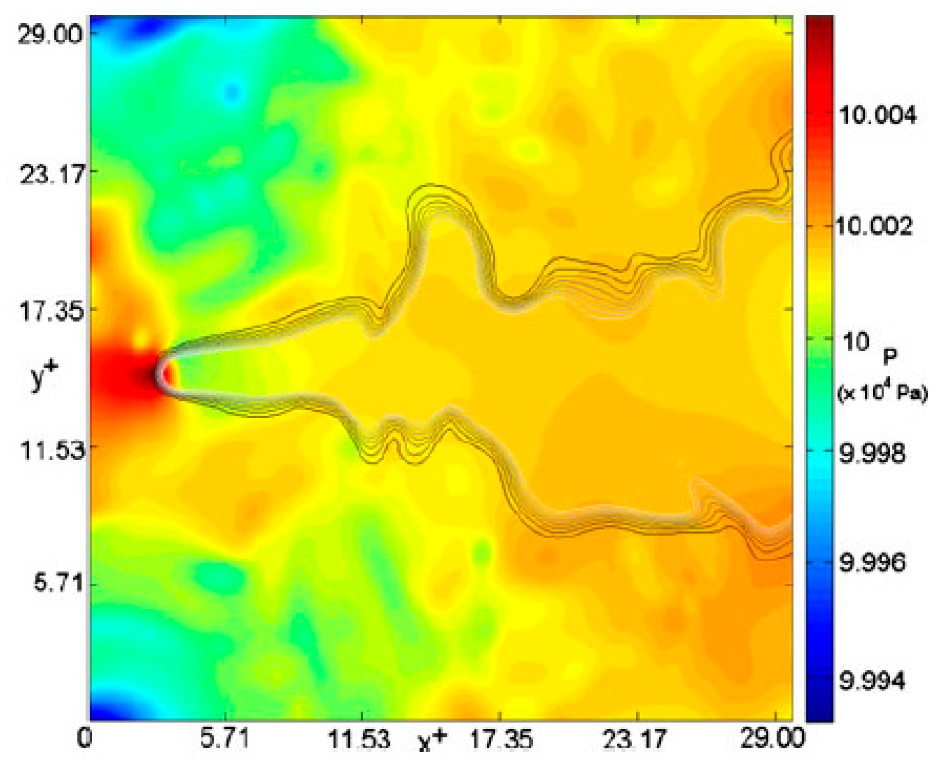
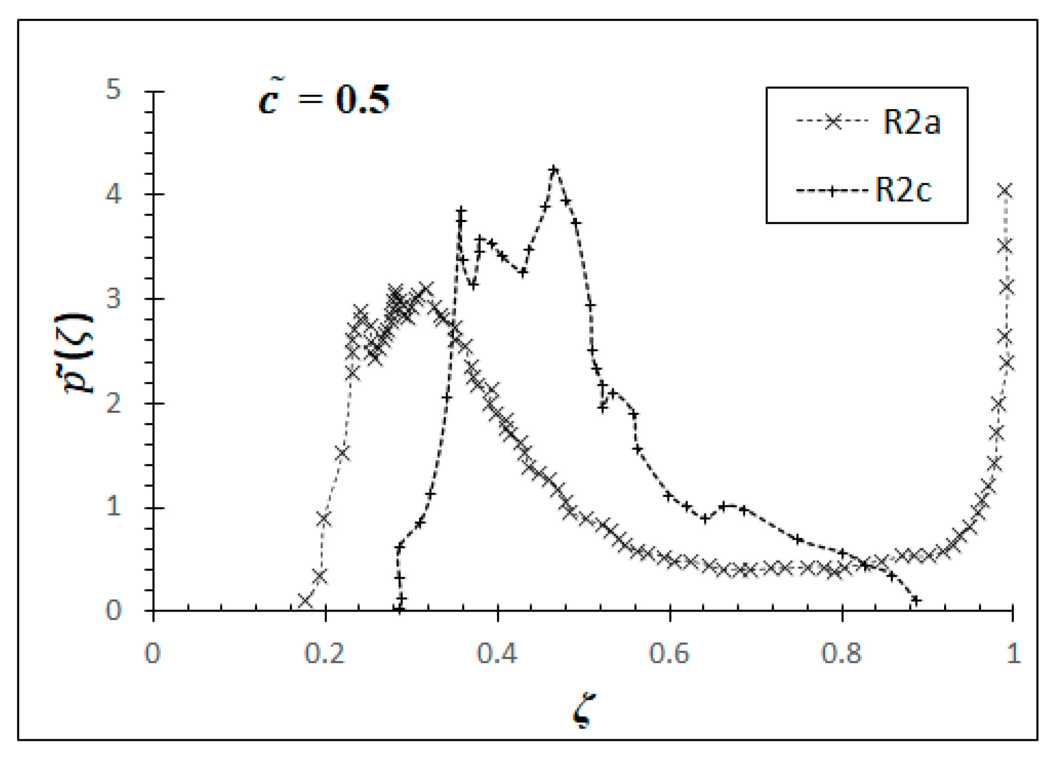
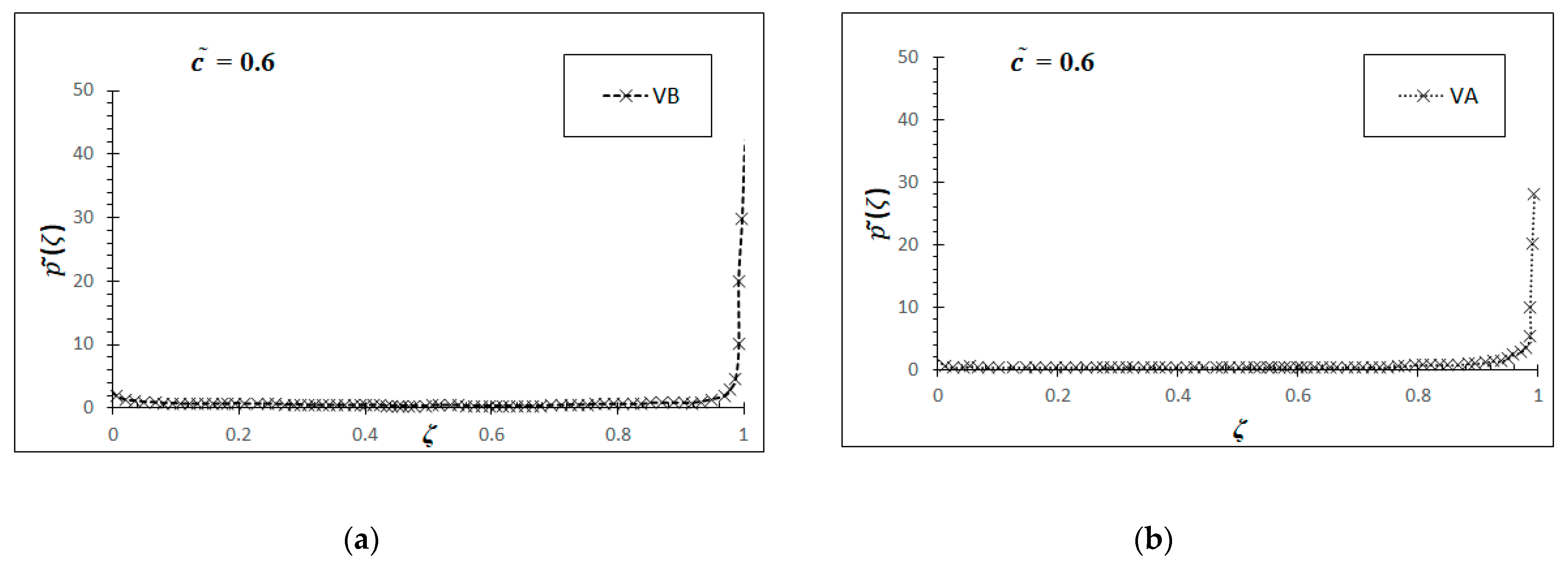
Figure 2 shows the V-flame from the experiment and DNS analysis for flames VA and VB. Figure 3 shows the distributions of the heat-release rate on a typical x–z plane for cases R2a and R2c. The change of the Favre PDF for the progress variable, $\tilde{c}$, with the sample space, $\zeta$, for flames R2a and R2c at $\tilde{c}$= 0.5 and flames VA and VB at $\tilde{c}$= 0.6 are shown in Figure 4 and Figure 5, respectively. 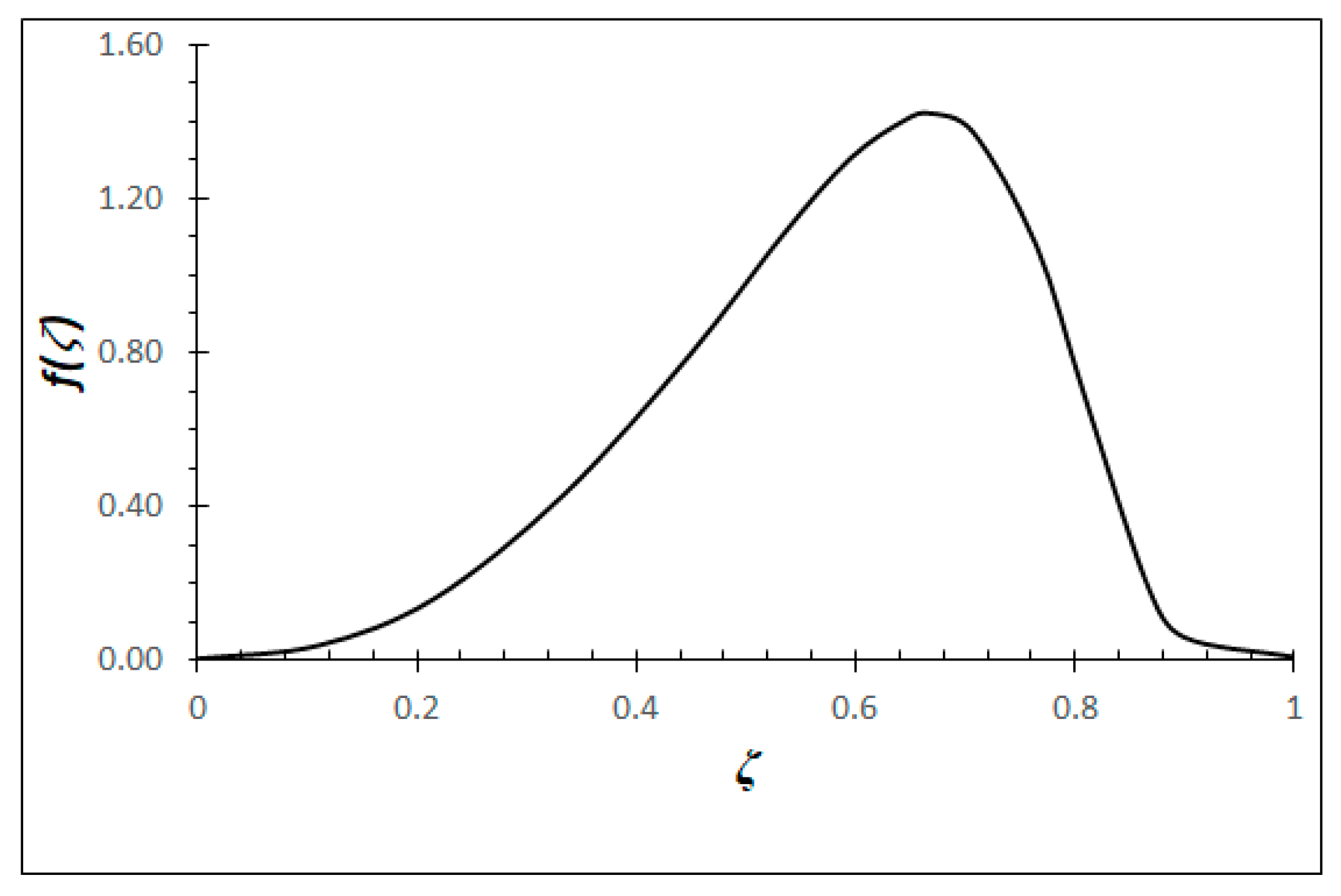Figure 6 shows the variation of f(ζ) in unstrained laminar flame for CH4–air of equivalence ratio 0.58. This curve is estimated using the PREMIX code [32] and the detailed chemical mechanism of GRI-3.0 [33].

4. Results and Discussion

The computational code used to determine the solution for the minimal least-squares norm, Equation (13), was developed at Moscow State University [26] where the mean scalar dissipation rate is computed from Equation (6) and f (ζ) obtained using an unstrained laminar flame. The PDF profiles are obtained from [17,19,20] using RANS simulations. The algebraic model that is given in Equation (10) specifies the initial solution. The regularisation parameter was set to be 1.001 to give the smallest value of the residual using 560 iterations.

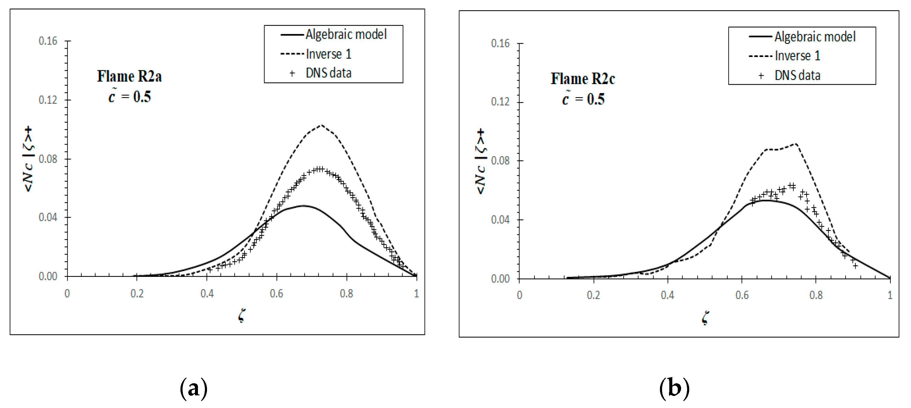
Figure 7 and Figure 8 show the change of the conditional mean scalar dissipation rate, $<N_c|\zeta >$, with the sample space, $\zeta$, at $\tilde{c}$= 0.5 for flames R2a and R2c and $\tilde{c}$ = 0.6 for V-flames. These results are obtained using the algebraic model, Equation (10), and the inverse model, Equation (13), and are compared with DNS results. These results are normalised using $S_L^0$ and ${\delta }_L^0$. As shown in the figures, both the inverse model Equation (13) and the algebraic model Equation (10) have predicted the peak and the general behaviour of$<N_c{|\zeta >}^{+}$ with the sample space $\zeta$.

The computed values of $<N_c{|\zeta >}^{+}$ obtained by the inverse model are over-predicted in the inner flame region for both flames. Far from this region, the agreement gradually improves for flames R2a and R2c. As noted earlier, the inverse model expects an initial estimate for the conditional mean dissipation rate and the model was found to be very sensitive to the initial estimate. For example, if the initial estimate is increased by 30%, then the model will deviate significantly from the DNS value, and this is the main limitation of this method. The computed values of $<N_c{|\zeta >}^{+}$ obtained by the algebraic model are in reasonable agreement with the DNS database for V-flames. The apparent reason is that these flames have a high Damköhler number as specified in (1). This agreement is consistent with the model limitation.

5. Sensitivity Analysis

The sensitivity to the initial solution is discussed in this section. It has been noticed that by providing the algebraic model Equation (10) as an initial solution for the conditional dissipation obtained by the inverse model Equation (13), the change of the conditional dissipation rate with the sample space ζ improves. Figure 9 compares the results obtained in the previous section (inverse 1) to the inverse model with the algebraic model as an initial estimation (inverse 2) and the DNS data. The comparison is shown for the flame R2a and R2c. These results are expected since the inverse model is known to be very sensitive to the initial solution. Therefore, to get a reasonably accurate solution for the conditional mean scalar dissipation rate, it is recommended to use the algebraic model as an initial guess for the inverse model.

6. Summary and Conclusions

In this study, an alternative model based on a mathematical approach is explored. The basic principle of this model is that the conditional mean dissipation rate, $<N_c|\zeta >$, is obtained by inverting the integral in Equation (1). This technique is commonly used in science and mathematics. Both the mathematical and the algebraic models were tested using two different DNS databases having different thermochemical and turbulence conditions. These databases consist of stoichiometric turbulent premixed flames of H2-air with preheated reactants at 700 K and lean turbulent premixed V-flames of CH4-air with preheated reactants at 600 K. It should be noted that the computed results were normalised using $S_L^0$ and ${\delta }_L^0$. The mathematical model has successfully predicted the peak and the typical profile of $<N_c{|\zeta >}^{+}$ with the sample space $\zeta$. However, the computed values were over-predicted in the inner flame region for both flames, where this inconsistency gradually improves outside the inner flame region. The main reason for this over-prediction is due to its sensitivity to the initial estimate. Nevertheless, the model prediction was acceptable and consistent with the algebraic model when a suitable initial solution was used.

It should be noted that the inverse model is based on a purely mathematical approach without any assumption of the turbulence and chemistry interaction. Hence, the inverse model’s usefulness is more general than other conditional scalar dissipation rate models and is expected to perform well for all flame regimes or LES modelling.