TS Fuzzy Robust Sampled-Data Control for Nonlinear Systems with Bounded Disturbances

Abstract

We investigate robust fault-tolerant control pertaining to Takagi–Sugeno (TS) fuzzy nonlinear systems with bounded disturbances, actuator failures, and time delays. A new fault model based on a sampled-data scheme that is able to satisfy certain criteria in relation to actuator fault matrix is introduced. Specifically, we formulate a reliable controller with state feedback, such that the resulting closed-loop-fuzzy system is robust, asymptotically stable, and able to satisfy a prescribed $H_{\infty }$ performance constraint. Linear matrix inequality (LMI) together with a proper construction of the Lyapunov–Krasovskii functional is leveraged to derive delay-dependent sufficient conditions with respect to the existence of robust $H_{\infty }$ controller. It is straightforward to obtain the solution by using the MATLAB LMI toolbox. We demonstrate the effectiveness of the control law and less conservativeness of the results through two numerical simulations.

1. Introduction

Since most real-world control systems require nonlinear modelling, it is crucial to design and develop appropriate controllers for nonlinear systems. Correspondingly, fuzzy Takagi–Sugeno (TS) models provide an effective way for the complex modelling of nonlinear systems with respect to linear input–output variables and fuzzy sets [1]. Indeed, TS fuzzy modelling is advantageous for designing and extending linear systems to nonlinear counterparts in a straightforward manner, which is an important fuzzy control methodology [2,3,4]. Examples of relevant studies include event-triggered control of fuzzy systems subject to networked delays [5] and delay-dependent stability criteria of TS systems with time delay [6].

Sampled-data feedback control is a practical method for realizing complex control schemes in various domains [7]. Driven by a periodic clock, a sampled-data controller performs sampling of the inputs, changing the states, and updating the outputs on the basis of the trigger of each clock edge. With the advent of digital technologies, sampled-data controllers demonstrated superiority over other control methods [8]. Over the years, sufficient stabilization conditions for dynamical systems with sampled-data control through input delays have been developed ([9,10,11]). Both stability and control performance requirements, such as the $H_{\infty }$ performance constraint, are equally important. In this respect, stabilization and $H_{\infty }$ control are of interest since $H_{\infty }$ control design allows for the control task to be formulated as a mathematical optimization problem for devising the controller solution ([11,12,13]).

On the other hand, a robust control system needs to keep the overall system stable and maintain a satisfactory performance when component failures occur [14]. In real-world environments, practical systems are subject to a variety of possible actuator faults, which include actuator aging, zero shift, electromagnetic interference, and nonlinear dead zones in different frequency fields. Therefore, it is essential to administer effective fault tolerance control measures and ensure high performance for dynamical systems. Several publications ([15,16] and references therein) studied uncertain reliable feedback $H_{\infty }$ control systems. Recently, Zhang et al. [17] investigated reliable control for fuzzy systems with time delays and actuator faults. In [18], the feedback-based reliable control of fuzzy systems with uncertain parameters was examined. Leveraging the Lyapunov stability and integral inequality methods, sufficient conditions were derived in [19] for stability analysis of fuzzy systems subject to actuator failures. However, most reliable control techniques are only implemented in linear fuzzy systems, while nonlinear fuzzy systems are not covered. From a practical point of view, nonlinearity together with actuator failure is important in fuzzy modelling.

The rationale of reachable set bounding is to identify an appropriate domain that can handle all reachable states of a dynamical system with respect to zero initial conditions with input disturbance conditions [20,21]. Moreover, systems have many real-life uses [22], such as gain minimization and control synthesis, and aircraft collision avoidance; therefore, it is significant to examine reachable dynamical systems, and several studies were published ([23,24]). To the best of our knowledge, however, research on sampled-data-based feedback reliable control with nonlinear TS fuzzy systems having actuator failures and time delays is yet to be comprehensively examined. This is the motivation of our current study, which makes the following contributions.

(i)

Reachable set bounding and fault-tolerant control design are properly considered for the first time in nonlinear fuzzy systems with bounded disturbances and actuator failures.

(ii)

On the basis of integral inequality and Lyapunov stability theory, a new set of sufficient conditions is derived to ensure that the proposed TS fuzzy model is asymptotically stable while satisfying the $H_{\infty }$ performance index.

(iii)

Demonstration and evaluation of effectiveness pertaining to the proposed method with two numerical simulations.

2. Description of Nonlinear Fuzzy System

A fuzzy local approximation technique can be utilized to construct a simplified fuzzy model with fuzzy rules [25]. We describe a nonlinear system as

$$\begin{array}{ccc}\hfill \dot{x}\left(t\right)& =& f\left(x\left(t\right)\right)+g\left(x\left(t\right)\right)u^f\left(t\right)+h\left(x\left(t\right)\right)w\left(t\right),\hfill \\ \hfill z\left(t\right)& =& f_z\left(x\left(t\right)\right)+g_z\left(x\left(t\right)\right)u^f\left(t\right)+h_z\left(x\left(t\right)\right)w\left(t\right),\hfill \end{array}$$

(1)

where $x\left(t\right)\in R^{n_x}$ is the state, $u^f\left(t\right)\in R^m$ is the control input of actuator fault, $w\left(t\right)\in R^{n_w}$ is the disturbance, and $z\left(t\right)\in R^{n_z}$ is the controlled output. $f(·),f_z(·),g(·),g_z(·),h(·)$ and $h_z(·)$ are nonlinear functions. Disturbance term $\overline{w}\left(t\right)$ is assumed to be bounded:

$$\begin{array}{c}\hfill w^T\left(t\right)w\left(t\right)\le {\overline{w}}^2,\end{array}$$

(2)

where $\overline{w}$ is a positive scalar. Now, we represent nonlinear functions $f\left(x\right(t\left)\right)$ and $f_z\left(x\left(t\right)\right)$ as:

$$\begin{array}{ccc}\hfill f\left(x\right(t\left)\right)& =& f_a\left(x\left(t\right)\right)+f_b\left(x\left(t\right)\right)\widehat{\varphi }\left(t\right),\hfill \\ \hfill f_z\left(x\left(t\right)\right)& =& f_{za}\left(x\left(t\right)\right)+f_{zb}\left(x\left(t\right)\right)\widehat{\varphi }\left(t\right),\hfill \end{array}$$

(3)

where $\widehat{\varphi }\left(t\right)={[{\widehat{\varphi }}_1\left(t\right){\widehat{\varphi }}_2\left(t\right)\cdots {\widehat{\varphi }}_s\left(t\right)]}^T.$ We obtain the following nonlinear system after simple manipulation. For more details, see [25].

$$\begin{array}{ccc}\hfill f\left(x\right(t\left)\right)& =& {\widehat{f}}_a\left(x\left(t\right)\right)+f_b\left(x\left(t\right)\right)\varphi \left(t\right),\hfill \\ \hfill f_z\left(x\left(t\right)\right)& =& {\widehat{f}}_{za}\left(x\left(t\right)\right)+f_{zb}\left(x\left(t\right)\right)\varphi \left(t\right),\hfill \end{array}$$

(4)

where ${\widehat{f}}_a\left(x\left(t\right)\right)=f_a\left(x\left(t\right)\right)+f_b\left(x\left(t\right)\right)E_{L}x\left(t\right),$ ${\widehat{f}}_{za}\left(x\left(t\right)\right)={\widehat{f}}_{za}\left(x\left(t\right)\right)+f_{zb}\left(x\left(t\right)\right)E_{L}x\left(t\right),$ $E_L={[E_{L1}^T{E}_{L2}^T\cdots E_{Ls}^T]}^T$. Then, we can represent nonlinear system (1) as

$$\begin{array}{ccc}\hfill \dot{x}\left(t\right)& =& {\widehat{f}}_a\left(x\left(t\right)\right)+g\left(x\left(t\right)\right)u^f\left(t\right)+h\left(x\left(t\right)\right)w\left(t\right)+f_b\left(x\left(t\right)\right)\varphi \left(t\right),\hfill \\ \hfill z\left(t\right)& =& {\widehat{f}}_{za}\left(x\left(t\right)\right)+g_z\left(x\left(t\right)\right)u^f\left(t\right)+h_z\left(x\left(t\right)\right)w\left(t\right)+f_{zb}\left(x\left(t\right)\right)\varphi \left(t\right),\hfill \end{array}$$

(5)

where $\varphi \left(t\right)={[{\varphi }_1\left(t\right){\varphi }_2\left(t\right)\cdots {\varphi }_s\left(t\right)]}^T$ and ${\varphi }_i\left(t\right)={\widehat{\varphi }}_i\left(t\right)-E{L}_{i}x\left(t\right)\in R,1\le i\le s$.

To model a nonlinear system (5), we constructed a class of TS fuzzy systems with local nonlinear representation. Plant Rule $\eta$: IF $v_1\left(t\right)$ is ${\Gamma }_{\eta 1}$ and $v_2\left(t\right)$ is ${\Gamma }_{\eta 2},\dots ,v_p\left(t\right)$ is ${\Gamma }_{\eta p}$ THEN

$$\begin{array}{ccc}\hfill \dot{x}\left(t\right)& =& A_{\eta }x\left(t\right)+B_{1\eta }w\left(t\right)+B_{2\eta }{u}^f\left(t\right)+G_{\eta }\varphi \left(t\right),\hfill \\ \hfill z\left(t\right)& =& C_{1\eta }x\left(t\right)+D_{1\eta }w\left(t\right)+D_{2\eta }{u}^f\left(t\right)+G_{z\eta }\varphi \left(t\right),\hfill \end{array}$$

(6)

where ${\Gamma }_{\eta j}$ are the fuzzy sets; $\eta =1,\dots ,r.$ r is the number of IF-THEN rules; $v\left(t\right)={[v_1\left(t\right)v_2\left(t\right)\dots v_p\left(t\right)]}^T\in R^{p\times 1}$ are the premise variables. We can obtain the final TS fuzzy model by using fuzzy inference with a singleton fuzzifier, product inference, and center average defuzzifier techniques as follows:

$$\begin{array}{ccc}\hfill \dot{x}\left(t\right)& =& \sum _{\eta =1}^r{\alpha }_{\eta }\left(t\right)\left[A_{\eta }x\left(t\right)+B_{1\eta }w\left(t\right)+B_{2\eta }{u}^f\left(t\right)+G_{\eta }\varphi \left(t\right)\right],\hfill \\ \hfill z\left(t\right)& =& \sum _{\eta =1}^r{\alpha }_{\eta }\left(t\right)\left[C_{1\eta }x\left(t\right)+D_{1\eta }w\left(t\right)+D_{2\eta }{u}^f\left(t\right)+G_{z\eta }\varphi \left(t\right)\right],\hfill \end{array}$$

(7)

where ${\alpha }_{\eta }\left(t\right)=\frac{w_{\eta }\left(\upsilon \left(t\right)\right)}{{\displaystyle \sum _{\eta =1}^r}{w}_{\eta }\left(\upsilon \left(t\right)\right)}$, with $w_{\eta }\left(\upsilon \left(t\right)\right)={\displaystyle \prod _{j=1}^p}{\beta }_{\eta j}\left({\upsilon }_j\left(t\right)\right)$, ${\beta }_{\eta j}\left({\upsilon }_j\left(t\right)\right)$ is the membership grade of ${\upsilon }_j\left(t\right)$ in ${\Gamma }_{\eta j}$ and ${\displaystyle \sum _{\eta =1}^r}{w}_{\eta }\left(v\left(t\right)\right)>0$, $w_{\eta }\left(v\left(t\right)\right)\ge 0,\eta =1,2,\cdots ,r$. Matrix ${\overline{A}}_{\eta }=A_{\eta }+\Delta A_{\eta }\left(t\right)$ is a time-varying matrix that denotes parametric uncertainty indicated by $\left[\Delta A_{\eta }\left(t\right)\right]=D_{\eta }{M}_{\eta }\left(t\right)\left[N_{a\eta }\right]$ where $D_{\eta }\mathrm{and}{N}_{a\eta }$ are known matrices with appropriate dimensions, and $M_{\eta }\left(t\right)$ is an unknown time-varying matrix with Lebesgue measurable elements bounded by $M_{\eta }^T\left(t\right)M_{\eta }\left(t\right)\le I_{\eta }.$ As such, we formulate System (7) with uncertainty

$$\begin{array}{ccc}\hfill \dot{x}\left(t\right)& =& \sum _{\eta =1}^r{\alpha }_{\eta }\left(t\right)\left[{\overline{A}}_{\eta }x\left(t\right)+B_{1\eta }w\left(t\right)+B_{2\eta }{u}^f\left(t\right)+G_{\eta }\varphi \left(t\right)\right],\hfill \\ \hfill z\left(t\right)& =& \sum _{\eta =1}^r{\alpha }_{\eta }\left(t\right)\left[C_{1\eta }x\left(t\right)+D_{1\eta }w\left(t\right)+D_{2\eta }{u}^f\left(t\right)+G_{z\eta }\varphi \left(t\right)\right].\hfill \end{array}$$

(8)

We denote the reachable set pertaining to the System (8) as:

$$\begin{array}{c}\hfill {\Re }_x=\{x\left(t\right)\in {\mathbb{R}}^n|x\left(t\right)\mathrm{and}\omega \left(t\right)\mathrm{satisfy}\left(8\right)\mathrm{and}\left(2\right)\}.\end{array}$$

(9)

Given a positive-definite symmetric matrix $P>0$, we define ellipsoid $\epsilon \left(P\right)$ that bounds reachable set (9) as:

$$\begin{array}{c}\hfill \epsilon \left(P\right)=\left\{x\right|x^{T}Px\le 1,x\in {\mathbb{R}}^n\}.\end{array}$$

(10)

In this study, we formulate a control law with minimal $H_{\infty }$ performance index in such a way that the closed loop control is robustly stable. As such a reliable fuzzy control law $u^f\left(t\right)$ is defined as $u^f\left(t\right)=Fu\left(t\right)$, where F is the actuator fault matrix. The sampled-data control input represented by variable time delay appears in the form [26,27] $u\left(t\right)=u_d\left(t_l\right)=u_d(t-(t-t_l))=u_d(t-\tau \left(t\right)),t_l\le t\le t_{l+1},\tau \left(t\right)=t-t_l,$ where $u_d$ is a discrete-time control signal and time-varying delay $0\le \tau \left(t\right)=t-t_l$ is piecewise linear with derivative $\dot{\tau }\left(t\right)=1,\mathrm{for} t\ne t_l$ where $t_l$ is the sampling instant. Consider sampling interval ${\tau }_l=t_{l+1}-t_l$ that may vary but is bounded. As such, $\tau \left(t\right)\le t_{l+1}-t_l={\tau }_l\le {\tau }_M$ for all $t_l$, where the maximal upper bound of sampling interval ${\tau }_l$ is ${\tau }_M$. On the basis of what is mentioned above, the sampled-data control input is $u\left(t\right)=Kx\left(t_l\right)$ with a time-varying piecewise continuous delay $\tau \left(t\right)=t-t_l.$ As a result, the fuzzy rule for overall control is in the following form:

Control Rule $\eta$: IF ${\upsilon }_1\left(t\right)$ is ${\Gamma }_{\eta 1}$ and ${\upsilon }_2\left(t\right)$ is ${\Gamma }_{\eta 2},\dots ,{\upsilon }_p\left(t\right)$ is ${\Gamma }_{\eta p}$ THEN $u^f\left(t\right)=F{K}_{\eta }x(t-\tau \left(t\right)),\eta =1,2,\dots r$, where $K_{\eta }$ is the control gain matrix. We can use the fuzzy inference with a singleton fuzzifier, product inference, and center average defuzzifier method to derive the following final control output:

$$\begin{array}{c}\hfill u^f\left(t\right)=\sum _{\eta =1}^r{\alpha }_{\eta }\left(t\right)\left[F{K}_{\eta }x(t-\tau \left(t\right))\right].\end{array}$$

(11)

Introducing the fuzzy inference method for control law (11), we can represent System (8) as

$$\begin{array}{cc}\hfill \dot{x}\left(t\right)& =\sum _{\eta =1}^r{\alpha }_{\eta }\left(t\right)\left[{\overline{A}}_{\eta }x\left(t\right)+B_{1\eta }w\left(t\right)+B_{2\eta }F{K}_{\eta }x(t-\tau \left(t\right))+G_{\eta }\varphi \left(t\right)\right],\hfill \\ \hfill z\left(t\right)& =\sum _{\eta =1}^r{\alpha }_{\eta }\left(t\right)\left[C_{1\eta }x\left(t\right)+D_{11\eta }w\left(t\right)+D_{12\eta }F{K}_{\eta }x(t-\tau \left(t\right))+G_{z\eta }\varphi \left(t\right)\right],\hfill \end{array}$$

(12)

where $\tau \left(t\right)$ is the time delay that is able to satisfy the condition $0\le \tau \left(t\right)\le {\tau }_M.$

Lemma 1

([27]). Consider a positive definite matrix $S\in {\mathbb{R}}^{n\times n},S=S^T>0$ and scalars $0<\tau \left(t\right)<{\tau }_M$ for vector function $x\left(t\right),$ we obtain

$$\begin{array}{cc}\hfill {\int }_{t-{\tau }_M}^t{\dot{x}}^T\left(s\right)S\dot{x}\left(s\right)\mathrm{d}s\le & -\frac{1}{{\tau }_M}{\left({\int }_{t-{\tau }_M}^t\dot{x}\left(s\right)\mathrm{d}s\right)}^{T}S\left({\int }_{t-{\tau }_M}^t\dot{x}\left(s\right)\mathrm{d}s\right),\hfill \end{array}$$

(13)

$$\begin{array}{cc}\hfill {\int }_{-{\tau }_M}^0{\int }_{t+\theta }^t{\dot{x}}^T\left(s\right)S\dot{x}\left(s\right)\mathrm{d}s\le & -\frac{2}{{\tau }_M^2}{\left({\int }_{-{\tau }_M}^0{\int }_{t+\theta }^t\dot{x}\left(s\right)\mathrm{d}s\mathrm{d}\theta \right)}^{T}S\left({\int }_{-{\tau }_M}^0{\int }_{t+\theta }^t\dot{x}\left(s\right)\mathrm{d}s\mathrm{d}\theta \right).\hfill \end{array}$$

(14)

3. Sampled-Data ${\mathit{H}}_{\infty }$ Control Design

We investigate the robust reliable stabilization of an uncertain fuzzy system with actuator failure. The main purpose is to derive the conditions for the existence of stabilizing state feedback reliable $H_{\infty }$ control law, such that, given a disturbance attenuation level $\gamma >0$, the resulting closed-loop system is robustly asymptotically stable. To facilitate the robust asymptotic stability of (12), consider the nominal form of a fuzzy system with $\Delta A_{\eta }\left(t\right)=0$ in which actuator fault matrix F is known in the form

$$\begin{array}{cc}\hfill \dot{x}\left(t\right)& =\sum _{\eta =1}^r{\alpha }_{\eta }\left(t\right)\left[A_{\eta }x\left(t\right)+B_{1\eta }w\left(t\right)+B_{2\eta }F{K}_{\eta }x(t-\tau \left(t\right))+G_{\eta }\varphi \left(t\right)\right],\hfill \\ \hfill z\left(t\right)& =\sum _{\eta =1}^r{\alpha }_{\eta }\left(t\right)\left[C_{1\eta }x\left(t\right)+D_{1\eta }w\left(t\right)+D_{2\eta }F{K}_{\eta }x(t-\tau \left(t\right))+G_{z\eta }\varphi \left(t\right)\right].\hfill \end{array}$$

(15)

More precisely, utilizing an appropriate Lyapunov–Krasovskii functional and Jensen’s inequality, we obtain sufficient conditions in LMIs with respect to the existence of reliable $H_{\infty }$ control design pertaining to nominal System (15) with known actuator failure. In addition, the result is extended to cover uncertain fuzzy System (12). The following theorem provides a sufficient condition for developing a reliable $H_{\infty }$ controller.

Theorem 1.

For given positive scalars ${\tau }_o,{\tau }_M,{\lambda }_1$ and known actuator fault matrix F, nonlinear continuous-time fuzzy System (15) is asymptotically stable with respect to a given disturbance attenuation level $\gamma >0,$ if there exist positive definite symmetric matrices $P,\widehat{Q},\widehat{R},\widehat{S},\widehat{U}$ and any matrix $Y_{\eta }$ with appropriate dimension in such a way that satisfies the following LMI:

$$\begin{array}{cc}\hfill {\psi }_{\eta }& =\left[\begin{array}{cc}{\left[{\widehat{\Theta }}_{m,n}\right]}_{8\times 8}\hfill & {\widehat{\Pi }}^T\hfill \\ *\hfill & -I\hfill \end{array}\right],1\le \eta \le r,\hfill \end{array}$$

(16)

where

$$\begin{array}{cc}\hfill {\widehat{\Theta }}_{1,1}& =\widehat{Q}+{\tau }_M\widehat{R}-\frac{\widehat{S}}{{\tau }_M}-2\widehat{U},{\widehat{\Theta }}_{1,2}=e^{-\beta {\tau }_M}\frac{\widehat{S}}{{\tau }_M},{\widehat{\Theta }}_{1,4}=X_1+{\lambda }_1{X}_1{A}_{\eta }^T),{\widehat{\Theta }}_{1,5}=X_1{E}^T,\hfill \\ \hfill {\widehat{\Theta }}_{1,6}& =2e^{-\beta {\tau }_M}\frac{\widehat{U}}{{\tau }_M},{\widehat{\Theta }}_{1,7}=2e^{-\beta {\tau }_M}\frac{\widehat{U}}{{\tau }_M},{\widehat{\Theta }}_{2,2}=-2e^{-\beta {\tau }_M}\frac{\widehat{S}}{{\tau }_M},{\widehat{\Theta }}_{2,3}=e^{-\beta {\tau }_M}\frac{\widehat{S}}{{\tau }_M},{\widehat{\Theta }}_{2,4}=Y_{\eta }^T{F}^T{B}_{2\eta }^T,{\widehat{\Theta }}_{3,3}=\hfill \\ & -e^{-\beta {\tau }_M}\widehat{Q}-e^{-\beta {\tau }_M}\frac{\widehat{S}}{{\tau }_M},{\widehat{\Theta }}_{4,4}={\tau }_M\widehat{S}+\frac{{\tau }_M^2}{2}\widehat{U}-2X_1,{\widehat{\Theta }}_{4,5}={\lambda }_1{G}_{\eta }{X}_2,{\widehat{\Theta }}_{4,8}=B_{1\eta }I,{\widehat{\Theta }}_{5,5}\hfill \\ & =-X_2,{\widehat{\Theta }}_{6,6}=-e^{-\beta {\tau }_M}\frac{R}{{\tau }_M}-2e^{-\beta {\tau }_M}\frac{\widehat{U}}{{\tau }_M^2},{\widehat{\Theta }}_{6,7}=-2e^{-\beta {\tau }_M}\frac{\widehat{U}}{{\tau }_M^2},{\widehat{\Theta }}_{7,7}=-e^{-\beta {\tau }_M}\frac{R}{{\tau }_M}-2e^{-\beta {\tau }_M}\frac{\widehat{U}}{{\tau }_M^2},{\widehat{\Theta }}_{8,8}=\hfill \\ & -{\gamma }^{2}I,\widehat{\Pi }=\left[C_{1\eta }{X}_1^T{D}_{12\eta }F{Y}_{\eta }{0}_{n,2n}{G}_{z1\eta }{X}_2^T{0}_{n,2n}{D}_{11\eta }\right].\hfill \end{array}$$

Proof. 

To arrive at the required result, consider the following Lyapunov–Krasovskii functional pertaining to nominal System (15) as follows:

$$\begin{array}{ccc}\hfill V(t,x(t\left)\right)& =& \sum _{i=1}^5{V}_i(t,x\left(t\right)),\hfill \end{array}$$

(17)

where

$$\begin{array}{ccc}\hfill V_1(t,x\left(t\right))& =& x^T\left(t\right)Px\left(t\right),\hfill \\ \hfill V_2(t,x\left(t\right))& =& {\int }_{t-{\tau }_M}^t{e}^{\beta (s-t)}{x}^T\left(s\right)Qx\left(s\right)ds,\hfill \\ \hfill V_3(t,x\left(t\right))& =& {\int }_{-{\tau }_M}^0{\int }_{t+\theta }^t{e}^{\beta (s-t)}{x}^T\left(s\right)Rx\left(s\right)dsd\theta ,\hfill \\ \hfill V_4(t,x\left(t\right))& =& {\int }_{-{\tau }_M}^0{\int }_{t+\theta }^t{e}^{\beta (s-t)}{\dot{x}}^T\left(s\right)S\dot{x}\left(s\right)dsd\theta ,\hfill \\ \hfill V_5(t,x\left(t\right))& =& {\int }_{-{\tau }_M}^0{\int }_{\theta }^0{\int }_{t+\lambda }^t{e}^{\beta (s-t)}{\dot{x}}^T\left(s\right)U\dot{x}\left(s\right)dsd\lambda d\theta .\hfill \end{array}$$

Through computing derivatives $\dot{V}(t,x\left(t\right))$ along the system trajectory, we obtain

$$\begin{array}{cc}\hfill {\dot{V}}_1(t,x\left(t\right))& =2x^T\left(t\right)P\dot{x}\left(t\right)-\beta V_1(t,x\left(t\right))+\beta V_1(t,x\left(t\right)),\hfill \\ \hfill {\dot{V}}_2(t,x\left(t\right))& =x^T\left(t\right)Qx\left(t\right)-e^{-\beta {\tau }_M}{x}^T(t-{\tau }_M)Qx(t-{\tau }_M)-\beta V_2(t,x\left(t\right)),\hfill \\ \hfill {\dot{V}}_3(t,x\left(t\right))& =x^T\left(t\right)\left({\tau }_{M}R\right)x\left(t\right)-e^{-\beta {\tau }_M}{\int }_{t-{\tau }_M}^t{x}^T\left(s\right)Rx\left(s\right)ds-\beta V_3(t,x\left(t\right)),\hfill \\ \hfill {\dot{V}}_4(t,x\left(t\right))& ={\dot{x}}^T\left(t\right)\left({\tau }_{M}S\right)\dot{x}\left(t\right)-e^{-\beta {\tau }_M}{\int }_{t-{\tau }_M}^t{\dot{x}}^T\left(s\right)S\dot{x}\left(s\right)ds-\beta V_4(t,x\left(t\right)),\hfill \end{array}$$

(18)

$$\begin{array}{cc}\hfill {\dot{V}}_5(t,x\left(t\right))& ={\dot{x}}^T\left(t\right)\left(\frac{{\tau }_M^2}{2}U\right)\dot{x}\left(t\right)-e^{-\beta {\tau }_M}{\int }_{-{\tau }_M}^0{\int }_{t+\theta }^t{\dot{x}}^T\left(s\right)U\dot{x}\left(s\right)dsd\theta -\beta V_5(t,x\left(t\right)).\hfill \end{array}$$

(19)

Combining Equations (17)–(19), we obtain

$$\begin{array}{cc}\hfill & \dot{V}(t,x\left(t\right))+\beta V(t,x\left(t\right))-\frac{\beta }{{\overline{w}}^2}{w}^T\left(t\right)w\left(t\right)\hfill \\ & =2x^T\left(t\right)P\dot{x}\left(t\right)+x^T\left(t\right)\left(\beta P+Q+{\tau }_{M}R\right)x\left(t\right)-e^{-\beta {\tau }_M}{x}^T(t-{\tau }_M)Qx(t-{\tau }_M)\hfill \\ & +{\dot{x}}^T\left(t\right)\left({\tau }_{M}S+\frac{{\tau }_M^2}{2}U\right)\dot{x}\left(t\right)-e^{-\beta {\tau }_M}{\int }_{t-{\tau }_M}^t{x}^T\left(s\right)Rx\left(s\right)ds\hfill \\ & -e^{-\beta {\tau }_M}{\int }_{t-{\tau }_M}^t{\dot{x}}^T\left(s\right)S\dot{x}\left(s\right)ds-e^{-\beta {\tau }_M}{\int }_{-{\tau }_M}^0{\int }_{t+\theta }^t{\dot{x}}^T\left(s\right)S\dot{x}\left(s\right)dsd\theta .\hfill \end{array}$$

(20)

By using Jensen’s inequality, integration in Equation (20) can be written as

$$\begin{array}{cc}\hfill -{\int }_{t-{\tau }_M}^t{x}^T\left(s\right)Rx\left(s\right)ds& =-{\int }_{t-{\tau }_M}^{t-\tau \left(t\right)}{x}^T\left(s\right)Rx\left(s\right)ds-{\int }_{t-\tau \left(t\right)}^t{x}^T\left(s\right)Rx\left(s\right)ds,\hfill \\ \hfill -{\int }_{t-{\tau }_M}^t{\dot{x}}^T\left(s\right)S\dot{x}\left(s\right)ds& =-{\int }_{t-{\tau }_M}^{t-\tau \left(t\right)}{\dot{x}}^T\left(s\right)S\dot{x}\left(s\right)ds-{\int }_{t-\tau \left(t\right)}^t{\dot{x}}^T\left(s\right)S\dot{x}\left(s\right)ds.\hfill \end{array}$$

Through the application of Lemma 1 onto each integral in the above equations, the following inequalities can be obtained:

$$\begin{array}{cc}\hfill -{\int }_{t-{\tau }_M}^{t-\tau \left(t\right)}{x}^T\left(s\right)Rx\left(s\right)ds& \le -\frac{1}{{\tau }_M}{\left[{\int }_{t-{\tau }_M}^{t-\tau \left(t\right)}x\left(s\right)ds\right]}^{T}R\left[{\int }_{t-{\tau }_M}^{t-\tau \left(t\right)}x\left(s\right)ds\right],\hfill \\ \hfill -{\int }_{t-\tau \left(t\right)}^t{x}^T\left(s\right)Rx\left(s\right)ds& \le -\frac{1}{{\tau }_M}{\left[{\int }_{t-\tau \left(t\right)}^{t}x\left(s\right)ds\right]}^{T}R\left[{\int }_{t-\tau \left(t\right)}^{t}x\left(s\right)ds\right],\hfill \\ \hfill -{\int }_{t-{\tau }_M}^{t-\tau \left(t\right)}{\dot{x}}^T\left(s\right)S\dot{x}\left(s\right)ds& \le -\frac{1}{{\tau }_M}{\left[x(t-\tau \left(t\right))-x(t-{\tau }_M)\right]}^{T}S\hfill \\ & \left[x(t-\tau \left(t\right))-x(t-{\tau }_M)\right],\hfill \\ \hfill -{\int }_{t-\tau \left(t\right)}^t{\dot{x}}^T\left(s\right)Sx\left(s\right)ds& \le -\frac{1}{{\tau }_M}{\left[x\left(t\right)-x(t-\tau (t\left)\right)\right]}^{T}S\left[x\left(t\right)-x(t-\tau (t\left)\right)\right],\hfill \\ \hfill -{\int }_{-{\tau }_M}^0{\int }_{t+\theta }^t{\dot{x}}^T\left(s\right)U\dot{x}\left(s\right)dsd\theta & \le {\alpha }_1^T\left(t\right)\left[\begin{array}{ccc}-2U& \frac{2}{{\tau }_M}U& \frac{2}{{\tau }_M}U\\ *& -\frac{2}{{\tau }_M^2}U& -\frac{2}{{\tau }_M^2}U\\ *& *& -\frac{2}{{\tau }_M^2}U\end{array}\right]{\alpha }_1\left(t\right),\hfill \end{array}$$

(21)

where ${\alpha }_1^T\left(t\right)=\left[x^T\left(t\right){\int }_{t-{\tau }_M}^{t-\tau \left(t\right)}{x}^T\left(s\right)ds{\int }_{t-\tau \left(t\right)}^t{x}^T\left(s\right)ds\right].$

In addition, for any matrix $P_1$ of appropriate dimension, the following equality holds:

$$\begin{array}{c}\hfill 2{\dot{x}}^T\left(t\right)P_1\left[A_{\eta }x\left(t\right)+B_{1\eta }w\left(t\right)+B_{2\eta }F{K}_{\eta }x(t-\tau \left(t\right))+G_{\eta }\varphi \left(t\right)-\dot{x}\left(t\right)\right]=0.\end{array}$$

(22)

To arrive at a convex condition for devising fuzzy controller, we need to perform transformation with respect to nonlinear term ${\overline{\varphi }}_i\left(t\right)$ [25]. Since ${\overline{\varphi }}_i\left(t\right)\in co\{E_{Li}x\left(t\right),E_{Ui}x\left(t\right)\}$, we obtain

$$\begin{array}{c}\hfill \left({\varphi }_i\left(t\right)\right)(E_{i}x\left(t\right)-{\varphi }_i\left(t\right))\ge 0\mathrm{for}1\le i\le s.\end{array}$$

(23)

By treating ${\Lambda }^{-1}$ from [25] as, ${\Lambda }^{-1}=\mathrm{diag}{[{\lambda }_1{\lambda }_2\cdots {\lambda }_s]}^{-1}=\mathrm{diag}[{\lambda }_1^{-1}{\lambda }_2^{-1}\cdots {\lambda }_s^{-1}],$ then

$$\begin{array}{cc}\hfill {\varphi }^T\left(t\right){\Lambda }^{-1}Ex\left(t\right)-{\varphi }^T\left(t\right){\Lambda }^{-1}\varphi \left(t\right)& =[{\lambda }_1^{-1}{\varphi }_i\left(t\right)\dots {\lambda }_s^{-1}{\varphi }_s\left(t\right)]E_i-\sum _{i=1}^s{\lambda }_i^{-1}{\varphi }_i^2\left(t\right),\hfill \\ \hfill & =\sum _{i=1}^s{\lambda }_i^{-1}\left({\varphi }_i\left(t\right)E_{i}x\left(t\right)-{\varphi }_i^2\left(t\right)\right),\hfill \\ \hfill & =\sum _{i=1}^s{\lambda }_i^{-1}\left({\varphi }_i\left(t\right)\left[E_{i}x\left(t\right)-{\varphi }_i\left(t\right)\right]\right).\hfill \end{array}$$

(24)

Combining (23) and (24) yields

$$\begin{array}{c}\hfill {\varphi }^T\left(t\right){\Lambda }^{-1}Ex\left(t\right)-{\varphi }^T\left(t\right){\Lambda }^{-1}\varphi \left(t\right)\ge 0.\end{array}$$

(25)

Combining Equations (20)–(25), we obtain

$$\begin{array}{cc}\hfill & \dot{V}(t,x\left(t\right))+\beta V(t,x\left(t\right))-\frac{\beta }{{\overline{w}}^2}{w}^T\left(t\right)w\left(t\right)\hfill \\ & \le 2x^T\left(t\right)(P+A_{\eta }^T{P}_1^T)\dot{x}\left(t\right)+x^T\left(t\right)\left(\beta P+Q-2U+{\tau }_{M}R\right)x\left(t\right)+2{\dot{x}}^T{P}_1\hfill \\ \hfill & G_{\eta }\varphi \left(t\right)-e^{-\beta {\tau }_M}{x}^T(t-{\tau }_M)Qx(t-{\tau }_M)+{\dot{x}}^T\left(t\right)\left({\tau }_{M}S+\frac{{\tau }_M^2}{2}U-2P_1\right)\dot{x}\left(t\right)\hfill \\ \hfill & +2{\dot{x}}^T{P}_1{B}_{2\eta }F{K}_{\eta }x(t-\tau \left(t\right))+2{\dot{x}}^T{P}_1{B}_{1\eta }w\left(t\right)+{\varphi }^T\left(t\right){\Lambda }^{-1}Ex\left(t\right)\hfill \\ \hfill & -{\varphi }^T\left(t\right){\Lambda }^{-1}\varphi \left(t\right)-e^{-\beta {\tau }_M}\frac{1}{{\tau }_M}{\left[x(t-\tau \left(t\right))-e^{-\beta {\tau }_M}x(t-{\tau }_M)\right]}^{T}S[x(t-\tau \left(t\right))\hfill \\ \hfill & -e^{-\beta {\tau }_M}x(t-{\tau }_M)]-e^{-\beta {\tau }_M}\frac{1}{{\tau }_M}{\left[x\left(t\right)-x(t-\tau (t\left)\right)\right]}^{T}S\left[x\left(t\right)-x(t-\tau (t\left)\right)\right]\hfill \\ \hfill & -e^{-\beta {\tau }_M}\frac{1}{{\tau }_M}{\left[{\int }_{t-{\tau }_M}^{t-\tau \left(t\right)}x\left(s\right)ds\right]}^T\left(R+\frac{2U}{{\tau }_M^2}\right)\left[{\int }_{t-{\tau }_M}^{t-\tau \left(t\right)}x\left(s\right)ds\right]-e^{-\beta {\tau }_M}\frac{1}{{\tau }_M}[{\int }_{t-\tau \left(t\right)}^t\hfill \\ \hfill & x\left(s\right)ds{]}^T\left(R+\frac{2U}{{\tau }_M^2}\right)\left[{\int }_{t-\tau \left(t\right)}^{t}x\left(s\right)ds\right]+x^T\left(t\right)e^{-\beta {\tau }_M}\left[\frac{2U}{{\tau }_M}\right]\left[{\int }_{t-\tau \left(t\right)}^{t}x\left(s\right)ds\right]\hfill \\ \hfill & +x^T\left(t\right)e^{-\beta {\tau }_M}\left[\frac{2U}{{\tau }_M}\right]\left[{\int }_{t-{\tau }_M}^{t-\tau \left(t\right)}x\left(s\right)ds\right]-e^{-\beta {\tau }_M}{\left[{\int }_{t-{\tau }_M}^{t-\tau \left(t\right)}x\left(s\right)ds\right]}^T\left[\frac{2U}{{\tau }_M^2}\right]\left[{\int }_{t-\tau \left(t\right)}^{t}x\left(s\right)ds\right].\hfill \end{array}$$

(26)

To study the $H_{\infty }$ performance with respect to the system, consider the following relation:

$$\begin{array}{c}\hfill J\left(t\right)={\int }_0^{\infty }[z^T\left(t\right)z\left(t\right)-{\gamma }^2{w}^T\left(t\right)w\left(t\right)]dt,\forall t>0.\end{array}$$

(27)

From (26) and subject to a zero initial condition, one can obtain $V\left(0\right)=0$ and $V(\infty )\ge 0$, then it is straightforward to indicate that

$$\begin{array}{ccc}\hfill J\left(t\right)& \le & {\int }_0^{\infty }\left[z^T\left(t\right)z\left(t\right)-{\gamma }^2{w}^T\left(t\right)w\left(t\right)+\dot{V}(t,x\left(t\right))+\beta V(t,x\left(t\right))-\frac{\beta }{{\overline{w}}^2}{w}^T\left(t\right)w\left(t\right)\right]dt,\hfill \\ & \le & {\int }_0^{\infty }{\xi }^T\left(t\right){\psi }_{\eta }\xi \left(t\right)dt,\hfill \end{array}$$

(28)

where ${\xi }^T\left(t\right)=\left[x^T\left(t\right)x^T(t-\tau \left(t\right))x^T(t-{\tau }_M)){\dot{x}}^T\left(t\right){\varphi }^T\left(t\right){\int }_{t-{\tau }_M}^{t-\tau \left(t\right)}{x}^T\left(s\right)ds{\int }_{t-\tau \left(t\right)}^t{x}^T\left(s\right)ds{w}^T\left(t\right)\right]$,

$$\begin{array}{cc}\hfill {\psi }_{\eta }& =\left[\begin{array}{cc}{\left[{\Theta }_{m,n}\right]}_{8\times 8}\hfill & {\Pi }^T\hfill \\ *\hfill & -I\hfill \end{array}\right],1\le \eta \le r,\hfill \end{array}$$

(29)

and

$$\begin{array}{cc}\hfill {\Theta }_{1,1}& =Q+{\tau }_{M}R-\frac{S}{{\tau }_M}-2U,{\Theta }_{1,2}=e^{-\beta {\tau }_M}\frac{S}{{\tau }_M},{\Theta }_{1,4}=P+A_{\eta }^T{P}_1^T,{\Theta }_{1,5}=E^T{\Lambda }^{-T},\hfill \\ \hfill {\Theta }_{1,6}& =2e^{-\beta {\tau }_M}\frac{U}{{\tau }_M},{\Theta }_{1,7}=2e^{-\beta {\tau }_M}\frac{U}{{\tau }_M},{\Theta }_{2,2}=-2e^{-\beta {\tau }_M}\frac{S}{{\tau }_M},{\Theta }_{2,3}=e^{-\beta {\tau }_M}\frac{S}{{\tau }_M},{\Theta }_{2,4}=K_{\eta }^T{F}^T{B}_{2\eta }^T{P}_1^T,\hfill \\ \hfill {\Theta }_{3,3}& =-Q-e^{-\beta {\tau }_M}\frac{S}{{\tau }_M},{\Theta }_{4,4}={\tau }_{M}S+\frac{{\tau }_M^2}{2}U-2P_1,{\Theta }_{4,5}=P_1{G}_{\eta },{\Theta }_{4,8}=2P_1{B}_{1\eta },\hfill \\ \hfill {\Theta }_{5,5}& =-{\Lambda }^{-1},{\Theta }_{6,6}=-e^{-\beta {\tau }_M}\frac{R}{{\tau }_M}-e^{-\beta {\tau }_M}\frac{2}{{\tau }_M^2}U,{\Theta }_{6,7}=-e^{-\beta {\tau }_M}\frac{2}{{\tau }_M^2}U,{\Theta }_{7,7}=-e^{-\beta {\tau }_M}\frac{R}{{\tau }_M}-e^{-\beta {\tau }_M}\frac{2}{{\tau }_M^2}U,\hfill \\ \hfill {\Theta }_{8,8}& =-{\gamma }^{2}I,\Pi =\left[C_{1\eta }{D}_{12\eta }F{K}_{\eta }{0}_{n,2n}{G}_{z1\eta }{0}_{n,2n}{D}_{11\eta }\right].\hfill \end{array}$$

To obtain a reliable $H_{\infty }$ feedback control gain matrix, take $P_1={\lambda }_{1}P$, where ${\lambda }_1$ is the designing parameter, and assume that $T=\mathrm{diag}\{X_1,X_1,X_1,X_1,\Lambda ,X_1,X_1\}$. Through the pre- and postmultiplication of (29) by $\mathrm{diag}\{T,I,I\}$, where $X_1=S,P=S^{-1}$ and by setting $\widehat{Q}=X_{1}Q{X}_1,\widehat{R}=X_{1}R{X}_1,\widehat{S}=X_{1}S{X}_1,\widehat{U}=X_{1}U{X}_1$ and $Y_{\eta }=K_{\eta }X$, LMI (16) can be obtained. With reference to LMI (16), if ${\psi }_{\eta }<0$, we arrive at $J\left(t\right)\le 0,i.e.,$

$$\begin{array}{cc}\hfill {\int }_0^{\infty }[z^T\left(t\right)z\left(t\right)-{\gamma }^2{w}^T\left(t\right)w\left(t\right)]dt& \le 0,\hfill \\ \hfill {\int }_0^{\infty }{z}^T\left(t\right)z\left(t\right)& \le {\gamma }^2{\int }_0^{\infty }{w}^T\left(t\right)w\left(t\right)dt.\hfill \end{array}$$

Hence, with respect to the definition of $H_{\infty }$, it can be concluded that fuzzy System (15) with known actuator failure matrix F is asymptotically stable with respect to a given performance attenuation level $\gamma >0$. This completes the proof.  □

Next, we derive a robust $H_{\infty }$ controller with respect to uncertain fuzzy System (12) on the basis of Theorem 1.

Theorem 2.

For given positive scalars ${\tau }_o,{\tau }_M,{\lambda }_1$ and known actuator fault matrix F, nonlinear continuous-time fuzzy System (12) is robustly asymptotically stable with a given disturbance attenuation level $\gamma >0,$ if there exist positive definite symmetric matrices $P,\widehat{Q},\widehat{R},\widehat{S},\widehat{U}$, any matrix $Y_{\eta }$ with appropriate dimension and positive scalar ϵ in such a way that satisfies the following LMI:

$$\begin{array}{cc}\hfill {\widehat{\psi }}_{\eta }& =\left[\begin{array}{ccc}{\psi }_{\eta }\hfill & {\Xi }_1^T\hfill & {\Xi }_2^T\\ *\hfill & -ϵI\hfill & 0\\ *\hfill & *\hfill & -ϵI\end{array}\right],1\le \eta \le r,\hfill \end{array}$$

(30)

where ${\Xi }_1=\left[Na\eta X_1^T{0}_{n,8n}\right],{\Xi }_2=\left[0_{n,3n}ϵ{\lambda }_1{D}_{\eta }^T{0}_{n,5n}\right]$ and the remaining parameters are defined in Theorem 1. As such, the state feedback control gain in (11) is given by $K_{\eta }=Y_{\eta }{X}^{-1}$.

Proof. 

The proof of Theorem 2 follows from Theorem 1. We replace $A_{\eta }$ with $A_{\eta }+\Delta A_{\eta }\left(t\right)$ in (22) to yield

$$\begin{array}{c}\hfill \dot{V}(t,x\left(t\right))\le {\xi }^T\left(t\right)({\psi }_{\eta }+{\Omega }_{\eta }\left(t\right))\xi \left(t\right),\end{array}$$

(31)

where

$$\begin{array}{c}\hfill {\Omega }_{\eta }\left(t\right)={\Xi }_1^T\left(t\right)M_{\eta }^T\left(t\right){\Xi }_2\left(t\right)+{\Xi }_2^T\left(t\right)M_{\eta }\left(t\right){\Xi }_1\left(t\right),\end{array}$$

Using S-procedure [27], we can represent the above inequality as

$$\begin{array}{c}\hfill {\Omega }_{\eta }\left(t\right)\le {ϵ}^{-1}{\Xi }_1^T\left(t\right)\Xi \left(t\right)+ϵ{\Xi }_2\left(t\right){\Xi }_2^T\left(t\right).\end{array}$$

Then Equation (31) becomes

$$\begin{array}{c}\hfill \dot{V}(t,x\left(t\right))\le {\xi }^T\left(t\right)\left[{\psi }_{\eta }+{ϵ}^{-1}{\Xi }_1^T\left(t\right)\Xi \left(t\right)+ϵ{\Xi }_2\left(t\right){\Xi }_2^T\left(t\right)\right]\xi \left(t\right).\end{array}$$

(32)

Now, by applying the Schur complement lemma [27], Inequality (32) is equivalent to LMI (30). This completes the proof.  □

Next, we design the robust reliable sampled-data $H_{\infty }$ controller when the actuator failure matrix F is not exactly known. The required state feedback controller is designed through the following theorem by using the conditions obtained in Theorem 2.

Theorem 3.

For given positive scalars ${\tau }_o,{\tau }_M,{\lambda }_1$ and unknown actuator fault matrix F, nonlinear continuous-time fuzzy System (12) is robust and asymptotically stable pertaining to sampled-data feedback control (11) with a given disturbance attenuation level $\gamma >0,$ if there exist positive definite symmetric matrices $P,\widehat{Q},\widehat{R},\widehat{S},\widehat{U}$, any matrix $Y_{\eta }$ with appropriate dimension and positive scalars $ϵ,{ϵ}_1$ in such a way that satisfies the following LMI:

$$\begin{array}{cc}\hfill {\Phi }_{\eta }& =\left[\begin{array}{cc}{\overline{\psi }}_{\eta }\hfill & \tilde{B}\hfill \\ *\hfill & -\widetilde{ϵ}\hfill \end{array}\right],1\le \eta \le r,\hfill \end{array}$$

(33)

where $\tilde{B}=\left[{ϵ}_1{\widehat{B}}^T{\widehat{Y}}_1^T\right],\widetilde{ϵ}=diag\{{ϵ}_{1}I,{ϵ}_{1}I\}$ and the remaining parameters are defined in Theorem 2.

Proof. 

Given an unknown actuator failure matrix F with respect to the fault condition, we can represent LMI (30) in Theorem 2 as

$$\begin{array}{c}\hfill {\Phi }_{\eta }={\overline{\psi }}_{\eta }+{\widehat{B}}^T\Delta {\widehat{Y}}_1+{\widehat{Y}}_1^T\Delta \widehat{B},\end{array}$$

(34)

where $\widehat{B}=\left[0_{n,5n}{B}_{2\eta }^T{0}_{n,2n}{D}_{12\eta }^T{0}_{n,2n}\right],{\widehat{Y}}_1=\left[0_n{F}_1{Y}_{\eta }{0}_{n,9n}\right]$ and ${\overline{\psi }}_{\eta }$ is achieved through the replacement of F by $F_0$ in ${\widehat{\psi }}_{\eta }$. In addition, through S-procedure [27] and (34), one can obtain

$$\begin{array}{c}\hfill {\Phi }_{\eta }={\overline{\psi }}_{\eta }+{ϵ}_1^{-1}\widehat{B}{\widehat{B}}^T+{ϵ}_1{\widehat{Y}}_1^T{\widehat{Y}}_1.\end{array}$$

(35)

Then by using Schur complement lemma [27], it is clear that (35) is equivalent to LMI (33). This completes the proof.  □

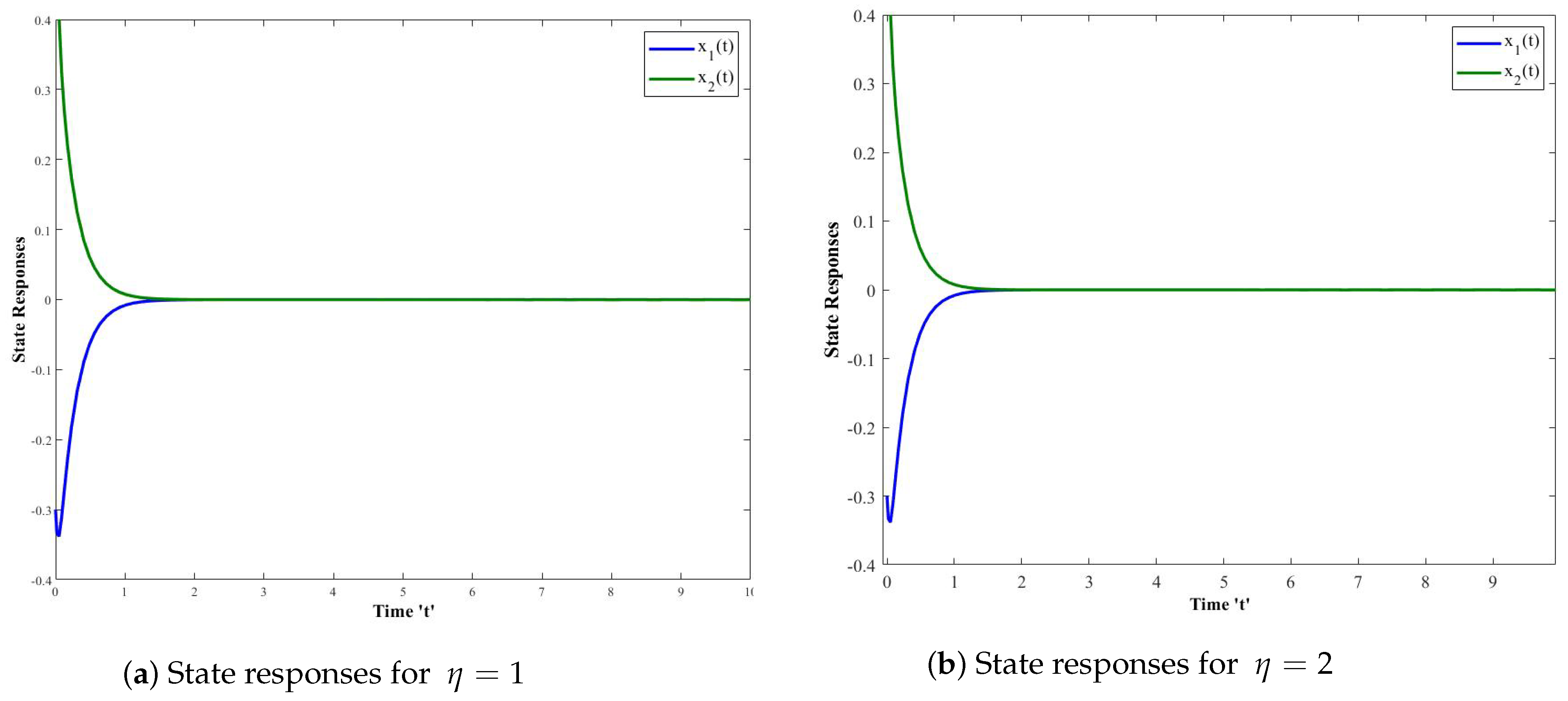
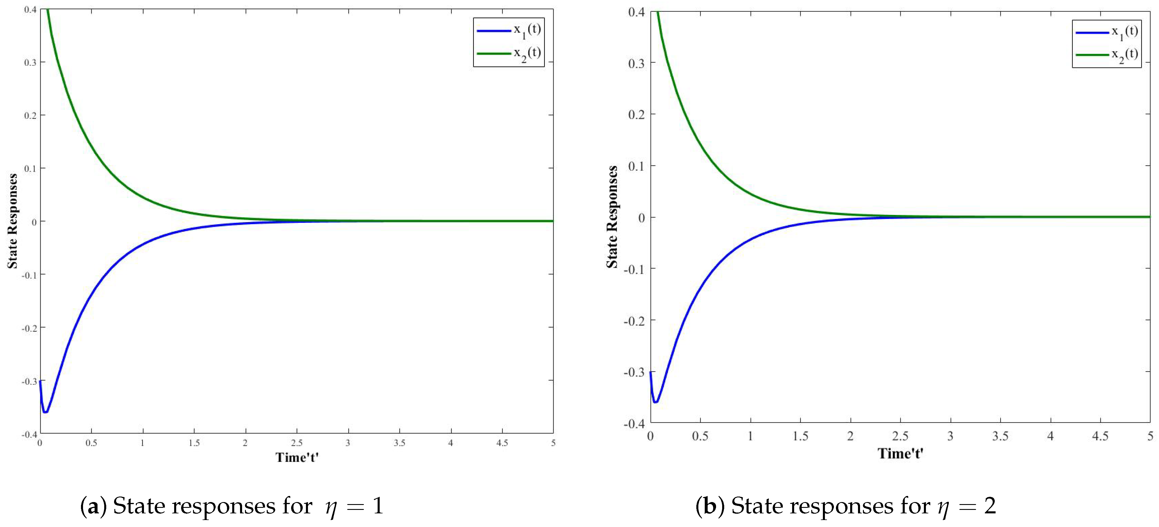
4. Numerical Simulations

Example 1.

To validate the proposed method, we consider the nonlinear model as

$$\begin{array}{cc}\hfill \left[\begin{array}{c}{\dot{x}}_1\hfill \\ {\dot{x}}_2\hfill \end{array}\right]& =\left[\begin{array}{c}0\hfill \\ 3si{n}^2\left(x_2\right)-1\hfill \end{array}\right]u+\left[\begin{array}{c}0\hfill \\ 1\hfill \end{array}\right]w\hfill \\ & +\left[\begin{array}{c}-2.6x_1-2x_2-2.4x_{1}si{n}^2\left(x_2\right)-x_{2}si{n}^2\left(x_2\right)\hfill \\ x_{1}co{s}^2\left(x_2\right)-4x_2+8x_{2}si{n}^2\left(x_2\right)+(6si{n}^2\left(x_2\right)-2)(1-cos\left(x_1\right))sin\left(x_1\right)\hfill \end{array}\right],\hfill \end{array}$$

where $x_1$ and $x_2$ are states of the nonlinear system with $x_1\in \{-\pi /2,\pi /2\}.$

Let

$$\begin{array}{cc}\hfill {\overline{f}}_a\left(x\left(t\right)\right)& =\left[\begin{array}{c}-2.6x_1-2x_2-2.4x_{1}si{n}^2\left(x_2\right)-x_{2}si{n}^2\left(x_2\right)\hfill \\ x_{1}co{s}^2\left(x_2\right)-4x_2+8x_{2}si{n}^2\left(x_2\right)+(6si{n}^2\left(x_2\right)-2)(1-cos\left(x_1\right))sin\left(x_1\right)\hfill \end{array}\right],\hfill \\ \hfill g\left(x\right(t\left)\right)& =\left[\begin{array}{c}0\hfill \\ 3si{n}^2\left(x_2\right)-1\hfill \end{array}\right],f_b\left(x\left(t\right)\right)=\left[\begin{array}{c}0\hfill \\ 3si{n}^2\left(x_2\right)-1\hfill \end{array}\right],h\left(x\left(t\right)\right)\left(t\right)={\left[\begin{array}{cc}0\hfill & 1\hfill \end{array}\right]}^T,\hfill \\ \hfill \varphi \left(t\right)& =(1-cos\left(x_1\right))sin\left(x_1\right).\hfill \end{array}$$

Membership functions are ${\alpha }_1\left(t\right)=si{n}^2\left(x_2\left(t\right)\right)$ and ${\alpha }_2\left(t\right)=co{s}^2\left(x_2\left(t\right)\right)$.

We can use the following two-rule TS fuzzy system with local nonlinear model to represent nonlinear System (15):

$$\begin{array}{cc}\hfill \dot{x}\left(t\right)& =\sum _{\eta =1}^2{A}_{\eta }x\left(t\right)+B_{1\eta }w\left(t\right)+B_{2\eta }{u}^f\left(t\right)+G_{\eta }\varphi \left(t\right),\hfill \\ \hfill z\left(t\right)& =\sum _{\eta =1}^2{C}_{1\eta }x\left(t\right)+D_{1\eta }w\left(t\right)+D_{2\eta }{u}^f\left(t\right)+G_{z\eta }\varphi \left(t\right)],\hfill \end{array}$$

where

$$\begin{array}{cc}\hfill A_1& =\left[\begin{array}{cc}-15.0\hfill & -12.5\hfill \\ -13.8\hfill & -18.6\hfill \end{array}\right],C_{11}=\left[\begin{array}{cc}-0.0739\hfill & 0\hfill \\ 0\hfill & -0.0160\hfill \end{array}\right],B_{11}=\left[\begin{array}{c}0\hfill \\ 1\hfill \end{array}\right],\hfill \\ \hfill A_2& =\left[\begin{array}{cc}-15.0\hfill & -11.5\hfill \\ -3.81\hfill & -17.6\hfill \end{array}\right],C_{12}=\left[\begin{array}{cc}-0.4097\hfill & 0\hfill \\ 0\hfill & -0.0104\hfill \end{array}\right],B_{12}=\left[\begin{array}{c}0\hfill \\ 1\hfill \end{array}\right],\hfill \end{array}$$

$B_{21}={\left[02\right]}^T,B_{22}={[0-1]}^T,G_1={\left[04\right]}^T,G_2={[0-2]}^T,D_{11}={[-0.30]}^T,D_{12}={[-0.30]}^T,D_{21}={[0-0.01]}^T,D_{22}={[-0.30]}^T,G_{z1}={[-0.010]}^T,G_{z2}={[-0.0160]}^T.$

The objective is to devise the sampled-data controller gain in (11) in such a way that closed-loop System (15) is asymptotically stable with $H_{\infty }$ performance attenuation level. In order to show this, the following cases are discussed.

Case I: Nominal System with fixed actuator fault:

We consider ${\tau }_M=0.6,\gamma =0.5$ and known actuator failure matrix $F=0.5$.

By using the MATLAB LMI toolbox, we solve LMIs in Theorem 1 and obtain the feasible solutions and gain matrices of state feedback sampled-data $H_{\infty }$ controller as $K_1=[-2.43570.4080],K_2=[-1.9819-0.0317]$ for disturbance input $w\left(t\right)=-0.005sin\left(t\right)$ and initial condition $x\left(0\right)={[0.2-0.2]}^T$. Simulation results for state responses pertaining to the nonlinear fuzzy model are presented in Figure 1. Specifically, Figure 1 depicts convergence of state responses of the nominal system within the equilibrium point.

Case II: Uncertain system with actuator fault not exactly known:

In this case, consider that the actuator fault occurs in the interval $diag\{0.2,0.3\}\le diag\{0.4,0.9\}$. We set the remaining parameters to those in case I, i.e., $N_{a1}=N_{a2}=0.1I,D_1=D_2=0.5$$\gamma =0.5,{\tau }_M=0.3$. As such, the reliable sampled-data $H_{\infty }$ controller gain matrices are obtained, namely, $K_1=[-0.2495-0.1022],K_2=[-1.6187-0.0182]$.Corresponding to the gain matrices, the state responses of the uncertain T-S fuzzy system are given in Figure 2. Figure 3 depicts that the reachable set of the system is contained in the ellipsoid. Figure 1 and Figure 2 show that the proposed nonlinear TS fuzzy model is asymptotically stable and satisfies $H_{\infty }$ performance even in the occurrence of uncertain parameters, actuator failures, and time delays. Thus, the proposed fault-tolerant controller is active to stabilize the proposed nonlinear fuzzy model.

Example 2.

Consider the TS fuzzy model without nonlinear functions. In order to provide a comparison example, we chose the same values as those of [28] for the system parameters that are presented below:

$$\begin{array}{cc}\hfill & A_1=\left[\begin{array}{cc}0& 1\\ -0.01& 0\end{array}\right],B_{21}={\left[\begin{array}{cc}0& 1\end{array}\right]}^T,B_{11}={\left[\begin{array}{cc}1& 0\end{array}\right]}^T,C_{11}=\left[\begin{array}{cc}0& 1\end{array}\right],\hfill \\ \hfill & D_{11}=D_{12}=D_{21}=D_{22}=0,A_2=\left[\begin{array}{cc}0& 1\\ -0.68& 0\end{array}\right],\hfill \\ \hfill & B_{22}={\left[\begin{array}{cc}0& 1\end{array}\right]}^T,B_{12}={\left[\begin{array}{cc}1& 0\end{array}\right]}^T,C_{12}=\left[\begin{array}{cc}0& 1\end{array}\right].\hfill \end{array}$$

Choosing value $F=0.5$ and solving the LMI in Theorem 1, we obtain the feasible solutions and gain matrices: $K_1=[-0.8132-0.9221]$ and $K_2=[-0.7987-0.96134]$. Under the gain matrices, the upper bound of ${\tau }_M$ and the minimal γ performance value are estimated and provided in

Table 1. Comparison outcomes.

	MAUB of ${\mathit{\tau }}_{\mathit{M}}$	${\mathit{\gamma }}_{min}$
Ref. [28]	0.2	1.2448
Our method	0.6	1.0162

.

On the basis of Table 1, we can conclude that our proposed method gives less conservative results compare with the result of [28].

5. Conclusions

Here, we studied the results of feedback fault-tolerant control of nonlinear fuzzy systems with time delay, bounded disturbances, and external disturbance. The fault-tolerant sampled-data $H_{\infty }$ controller design based on the Lyapunov method and Jensen’s integral inequality was presented in the form of LMIs, which can be solved by using standard numerical toolbox. Moreover, novel sufficient conditions were derived to ensure that the asymptotic stability pertaining to the fuzzy nonlinear systems subject to time-delay, bounded disturbances and component failures. Lastly, two numerical examples illustrated the effectiveness of the considered study.

References

1. Cai, X.; Zhong, S.; Wang, J.; Shi, K. Robust H control for uncertain delayed T-S fuzzy systems with stochastic packet dropouts. Appl. Math. Comput. 2020, 385, 125432. [Google Scholar] [CrossRef]
2. Senan, S. An Analysis of global stability of Takagi Sugeno fuzzy cohengrossberg neural networks with time delays. Neural Process. Lett. 2018, 10, 1–12. [Google Scholar]
3. Senthilraj, S.; Raja, R.; Zhu, Q.; Samidurai, R. Effects of leakage delays and impulsive control in dissipativity analysis of Takagi-Sugeno fuzzy neural networks with randomly occurring uncertainties. J. Frankl. Inst. 2017, 354, 3574–3593. [Google Scholar]
4. Shen, H.; Xiang, M.; Huo, S.; Wu, Z.G.; Park, J.H. Finite-time H asynchronous state estimation for discrete-time fuzzy Markov jump neural networks with uncertain measurements. Fuzzy Sets Syst. 2019, 356, 113–128. [Google Scholar] [CrossRef]
5. Pan, Y.; Yang, G.H. Event-based output tracking control for fuzzy networked control systems with network-induced delays. Appl. Math. Comput. 2019, 346, 513–530. [Google Scholar] [CrossRef]
6. Souza, F.O.; Campos, V.C.S.; Palhares, R.M. On delay-dependent stability conditions for Takagi-Sugeno fuzzy systems. J. Frankl. Inst. 2014, 351, 3707–3718. [Google Scholar] [CrossRef]
7. Zhang, H.; Feng, G.; Yan, H.; Chen, Q. Sampled-data control of nonlinear networked systems with time-delay and quantization. Int. J. Robust Nonlinear Control 2016, 26, 919–933. [Google Scholar] [CrossRef]
8. Cheng, J.; Wang, B.; Park, J.H.; Kang, W. Sampled-data reliable control for T-S fuzzy semi-Markovian jump system and its application to single link robot arm model. IET Control. Theory Appl. 2017, 11, 1904–1912. [Google Scholar] [CrossRef]
9. Liu, W.; Lim, C.C.; Shi, P.; Xu, S. Sampled-data fuzzy control for a class of nonlinear systems with missing data and disturbances. Fuzzy Sets Syst. 2017, 306, 63–86. [Google Scholar] [CrossRef]
10. Liu, Y.; Park, J.H.; Guo, B.Z.; Shu, Y. Further results on stabilization of chaotic systems based on fuzzy memory sampled-data control. IEEE Trans. Fuzzy Syst. 2018, 26, 1040–1045. [Google Scholar] [CrossRef]
11. Su, L.; Shen, H. Mixed H and passive synchronization for complex dynamical networks with sampled-data control. Appl. Math. Comput. 2015, 259, 931–942. [Google Scholar]
12. Wang, Q.; Zhang, Y.; Dong, C.; Jiang, Y. H output tracking control for flight control systems with time-varying delay. Chin. J. Aeronaut. 2013, 26, 1251–1258. [Google Scholar]
13. Wu, Z.G.; Park, J.H.; Su, H.; Song, B.; Chu, J. Mixed H and passive filtering for singular systems with time delays. Signal Process. 2013, 93, 1705–1711. [Google Scholar] [CrossRef]
14. Liu, Y.; Niu, Y.; Zou, Y.; Karimi, H.R. Adaptive sliding mode reliable control for switched systems with actuator degradation. IET Control Theory Appl. 2015, 9, 1197–1204. [Google Scholar] [CrossRef]
15. Hu, H.; Jiang, B.; Yang, H. Reliable guaranteed-cost control of delta operator switched systems with actuator faults: Mode-dependent average dwell-time approach. IET Control. Theory Appl. 2016, 10, 17–23. [Google Scholar] [CrossRef]
16. Shen, H.; Wang, Y.; Xia, J.; Park, J.H.; Wang, Z. Fault-tolerant leader-following consensus for multi-agent systems subject to semi-Markov switching topologies: An event-triggered control scheme. Nonlinear Anal. Syst. 2019, 34, 92–107. [Google Scholar] [CrossRef]
17. Zhang, J.X.; Yang, G.H. Fuzzy adaptive fault-tolerant control of unknown nonlinear systems with time-varying structure. IEEE Trans. Fuzzy Syst. 2019, 27, 1904–1916. [Google Scholar] [CrossRef]
18. Sun, S.; Zhang, H.; Wang, Y.; Cai, Y. Dynamic output feedback-based fault-tolerant control design for T-S fuzzy systems with model uncertainties. ISA Trans. 2018, 81, 32–45. [Google Scholar] [CrossRef] [PubMed]
19. Sun, S.; Wang, Y.; Zhang, H.; Xie, X. A new method of fault estimation and tolerant control for fuzzy systems against time-varying delay. Nonlinear Anal. Hybrid Syst. 2020, 38, 100942. [Google Scholar] [CrossRef]
20. Feng, Z.; Lam, J. On reachable set estimation of singular systems. Automatica 2015, 52, 146–153. [Google Scholar] [CrossRef]
21. Poongodi, T.; Saravanakumar, T.; Mishra, P.P.; Zhu, Q. Extended dissipative control for Markovian jump time-delayed systems with bounded disturbances. Math. Probl. Eng. 2020, 2020, 5685324. [Google Scholar] [CrossRef]
22. Feng, Z.; Zheng, W.X. On reachable set estimation of delay Markovian jump systems with partially known transition probabilities. J. Frankl. Inst. 2016, 353, 3835–3856. [Google Scholar] [CrossRef]
23. Lam, J.; Zhang, B.; Chen, Y.; Xu, S. Reachable set estimation for discrete-time linear systems with time delays. Int. J. Robust Nonlinear Control 2015, 25, 269–281. [Google Scholar] [CrossRef]
24. Sheng, Y.; Shen, Y. Improved reachable set bounding for linear time-delay systems with disturbances. J. Frankl. Inst. 2016, 353, 2708–2721. [Google Scholar] [CrossRef] [Green Version]
25. Dong, J.; Wang, Y.; Yang, G.H. Control synthesis of continuous-time T-S fuzzy systems with local nonlinear models. IEEE Trans. Syst. Man, Cybern. Part B (Cybern.) 2009, 39, 1245–1258. [Google Scholar] [CrossRef] [PubMed]
26. Yoneyama, J. Robust sampled-data stabilization of uncertain fuzzy systems via input delay approach. Inf. Sci. 2012, 198, 169–176. [Google Scholar] [CrossRef]
27. Saravanakumar, T.; Muoi, N.H.; Zhu, Q. Finite-time sampled-data control of switched stochastic model with non-deterministic actuator faults and saturation nonlinearity. J. Frankl. Inst. 2020, 357, 13637–13665. [Google Scholar] [CrossRef]
28. Zhang, H.; Yang, J.; Su, C.Y. T-S fuzzy-model-based robust H design for networked control systems with uncertainties. IEEE Trans. Ind. Inform. 2007, 3, 289–301. [Google Scholar] [CrossRef]
Figure 1. Simulation results for nonlinear TS fuzzy system with absence of uncertain parameters.
Computation 09 00132 g001
Figure 2. Simulation results for nonlinear uncertain TS fuzzy system.
Computation 09 00132 g002
Figure 3. Bounding ellipsoid and reachable set of TS fuzzy system with actuator fault.
Computation 09 00132 g003