Abstract
Explicit expressions are obtained for sensitivity coefficients to separately estimate temperature-dependent thermophysical properties, such as specific heat and thermal conductivity, in two-dimensional inverse transient heat conduction problems for bodies with irregular shape from temperature measurement readings of a single sensor inside the body. The proposed sensitivity analysis scheme allows for the computation of all sensitivity coefficients in only one direct problem solution at each iteration with no need to solve the sensitivity and adjoint problems. In this method, a boundary-fitted grid generation (elliptic) method is used to mesh the irregular shape of the heat conducting body. Explicit expressions are obtained to calculate the sensitivity coefficients efficiently and the conjugate gradient method as an iterative gradient-based optimization method is used to minimize the objective function and reach the solution. A test case with different initial guesses and sensor locations is presented to investigate the proposed inverse analysis.
1. Introduction
The accuracy of the numerical simulation of heat transfer problems relies significantly on the accuracy of data, including, among others, the thermophysical properties such as the thermal conductivity and the specific heat of heat-conducting body. If, no a priori information on the thermophysical properties is available, inverse methods, as inexpensive alternatives to expensive experiments with sophisticated instruments, may be employed to estimate the unknown properties accurately. The inverse methods are widely used to estimate the thermal conductivity and the specific heat. Sawaf et al. [1] estimated linearly temperature-dependent thermal conductivity and specific heat capacity for an orthotropic solid using an inverse analysis. The Levenberg–Marquardt iterative procedure is used to minimize the objective function. Flach and Özişik [2] employed an inverse analysis to estimate spatially varying thermal conductivity and heat capacity per unit volume of an one-dimensional slab using the Levenberg–Marquardt method. Talukdar et al. [3] used ant colony optimization algorithm for the estimation of temperature-dependent thermal conductivity and specific heat. Mohebbi et al. [4] derived explicit sensitivity coefficients to estimate the linearly temperature-dependent thermal conductivity in steady-state heat conduction problems using an inverse analysis. The conjugate-gradient method is used as a minimization method to minimize the objective function and estimate the unknown parameters. Liu [5] used a hybrid method based on a combination of the modified genetic algorithm and Levenberg–Marquardt method to identify simultaneously the fluid thermal conductivity and heat capacity for a transient inverse heat transfer problem. Czél et al. [6] presented an artificial neural network based solution of the inverse heat conduction problem to simultaneous identification of temperature-dependent volumetric heat capacity and thermal conductivity function of a solid.
However, in the literature, it can be noticed that there are still major limitations on the problems and the proposed methods to address the parameter estimation problems, including
- -
- The steady-state or transient heat conduction problems are concerned with regular bodies only (inability to consider the irregular bodies) and the heat conduction equation is solved using the traditional finite-difference method.
- -
- Most of the boundary conditions considered are associated with either a constant temperature (Dirichlet boundary condition) or an insulated surface. Hence, the Neumann and Robin boundary condition types are not addressed.
- -
- Most of the earlier works have been limited to the one-dimensional heat conduction problems.
Therefore, a sufficiently accurate general methodology for solving transient heat conduction problems in the presence of temperature-dependent thermophysical properties, which can handle a general 2D domain and a variety of boundary conditions, is required. This study is concerned with direct and inverse transient heat conduction problems in general 2D domains with different boundary conditions.
The inverse heat transfer problems are mathematically challenging problems due to their ill-posed nature. They are inherently unstable and very sensitive to noise and special methods are required to treat them. Among such methods are iterative regularization methods [7,8]. In these methods, the original objective function expression, defined as a nonlinear least-square formulation, is not modified and the minimization of the objective function is performed by a gradient-based minimization method such as conjugate-gradient method or steepest descent method and the discrepancy principle can be used as a criterion to stop the iteration process and obtain a reasonably stable solution. As this study is concerned with a parameter estimation problem, the gradient of the objective function with respect to the unknown parameters (as needed in gradient-based minimization methods) can be computed by using the finite-difference method (by additional direct problem solutions and forming the sensitivity matrix) or adjoint method. Both methods involve an increase in computational cost. Moreover, the adjoint method has its own mathematical complexity. In this study, however, using the obtained explicit sensitivity coefficients, the gradient of the objective function can be computed in only one direct problem solution at each iteration, thereby decreasing the computational cost significantly.
2. Governing Equation
The heat conducting body shown in Figure 1a is made of a material whose thermal conductivity and specific heat are linearly temperature-dependent variables, namely and where , , , and are constant. The density of the body is and the body is initially at the temperature . For the time , a time wise varying heat flux is applied at the boundary surface . Convective heat transfer is imposed on boundary surfaces with corresponding heat transfer coefficients and surrounding temperatures .
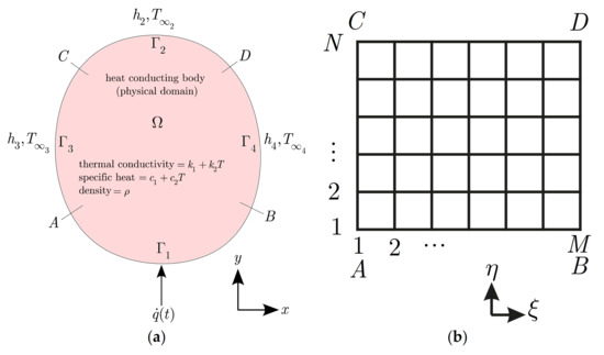
Figure 1.
Arbitrarily shaped two dimensional heat-conducting body (physical domain) subjected to a timewise varying heat flux on surface and convective heat transfer on surfaces (a) and the corresponding computational domain (b).
For this problem, the two-dimensional transient heat conduction equation with no heat generation is
for the linearly temperature-dependent thermal conductivity and the specific heat, namely and , Equation(1) is expressed as
by simplifying Equation (2), we get
The boundary and initial conditions are
where is the time. Since the and physical domain (the geometry of the heat-conducting body) is irregular, it is mapped onto a regular one (the and computational domain). The elliptic grid generation method (by solving two Laplace equations and ) is used to mesh the physical domain. Then the transient heat conduction equation and its associated boundary and initial conditions can be transformed from the () to the () variables [7,9,10,11]. The transformation gives
where
are the coefficients obtained from the elliptic grid generation method. By simplifying Equation (7), we get
The transformed boundary and initial conditions become
where is the initial condition rewritten in terms of the variables and . The derivatives appearing in the transformed heat conduction equation, Equation (9), can be discretized in the regular computational domain using the finite-difference method, as follows (assuming )
where . One-sided forward and one-sided backward relations should be used to discretize the boundary condition equations. Using forward-time-central-space (FTCS) discretization and the relations in Equation (15), and employing an explicit approach, we can approximate the differential Equation (9) as follows
where and are the time step and the time level, respectively. By considering the stability criterion for the solution of Equation (16), a time-marching procedure can be used to obtain . In other words, the nodal temperatures at the time level , , can be determined from the knowledge of nodal temperatures at the previous time level , , as follows
3. The Inverse Analysis
3.1. Objective Function
The objective of this study is to separately estimate the linearly temperature-dependent thermophysical properties such as the thermal conductivity and the specific heat using the transient readings of a single sensor placed at the point inside the body. To do so, using an inverse analysis the square of the difference between the estimated temperatures at the sensor place,, computed from the solution of the direct heat conduction problem using the estimated thermophysical properties and the measured temperatures over the time domain is minimized. This can be mathematically expressed as
where is a positive constant and can be considered as The inverse analysis is used to minimize the following objective function expression:
3.2. Sensitivity Analysis
The calculation of the gradient of the objective function defined by Equation (19) with respect to the unknown variables, , , , and is needed in the inverse problem. Thus, we can write
where . In Equation (20), () are called the sensitivity coefficients and can be obtained by differentiating the obtained expression for in Equation (17) with respect to , , , and , as follows
where
where , , , , , , , , and are computed using the finite-difference expressions associated with the sensor place, at the time , . By considering Equations (21)–(24), it can be seen that the inverse problem of estimating and is linear (as the sensitivity coefficient expressions are independent of and ) and the inverse problem of estimating and is nonlinear (as the sensitivity coefficient expressions depend on and ).
Moreover, it can be noticed that all sensitivity coefficients () can be computed in only one single direct problem solution without the need for solving sensitivity and adjoint problems. The sensitivity matrix can be explicitly written as
and
3.3. The Conjugate Gradient Method (CGM)
In this study, the conjugate gradient optimization method is used to solve the inverse heat transfer problem. The objective function given by Equation (19) is minimized by searching along the direction of descent using a search step length .
where are parameters to be estimated. The direction of descent of the current iteration is obtained as a linear combination of the direction of descent of the previous iteration and the gradient direction . Therefore,
The Polak–Ribiere formula [12] is used to compute the conjugation coefficient:
The search step-length is given as follows [7]
The parameter update in the conjugate-gradient or steepest-descent methods can be written as
If then which may result in a negative thermophysical property which is unacceptable. So, the objective function term (least squares norm) is multiplied by the constant to prevent a negative thermophysical property. The multiplication of the objective function by a constant does not change the optimal solution. Then, from Equation (20), the gradient of the objective function, , is also multiplied by . As the sensitivity coefficients all are multiplied by the constant , from Equation (31) we find that the search-step length is multiplied by . Therefore, by introducing the constant the term will be of its value without considering the constant ( is obtained from ). This way the updated parameter will be positive and the iteration process can continue. we can interpret this matter as follows:
The incorporation of the constant into the objective function definition has no effect on both the optimal solution and the gradient and only decreases the step-length as of its value when the constant is not considered (i.e., we initiate the iterative process with a smaller step-length):
The value of is a convention based on numerical experience which works well for the parameter estimation problems. In this study, until , we still get negative thermophysical property and the iteration process is terminated and hence is chosen to initiate the iterations.
Optimization Algorithm
The following algorithm presents the direct and inverse analysis steps used to estimate the linearly temperature-dependent thermal conductivity and the specific heat separately. To do so, either two parameters and for the thermal conductivity or two parameters and for the specific heat are estimated simultaneously. In other words, it is assumed that is known when estimating , and vice versa. Simultaneous estimation of all parameters , , , and is not considered in this study.
- -
- Estimation of (assuming is known):
- Specify the physical domain, the boundary and initial conditions, the thermophysical properties, and the measured temperatures at the sensor place and the time (), .
- Generate the boundary-fitted grid over the heat-conducting body using the elliptic grid generation method.
- Solve the direct problem to obtain the temperature values at the sensor place and the time (), , through solving Equations (7)–(14).
- Using Equation (19), compute the objective function ().
- If value of the objective function obtained in step 4 is less than the specified stopping criterion, the optimization is finished. Otherwise, go to step 6.
- Compute the sensitivity matrix from Equation (26).
- Compute the gradient directions from Equation (20).
- Compute the conjugation coefficients Equation (30). For , set .
- Compute the directions of descent from Equation (29).
- Compute the search step-length from Equation (31).
- From Equation (28), evaluate the new values for , namely .
- With new value for repeat the steps 6 to 11 for .
- Set the next iteration () and return to the step 2.
- -
- Estimation of (assuming is known):Repeat the steps 1 to 13 given above for the simultaneous estimation of and .
3.4. Stopping Criterion
If there are no errors in the temperature measurements, then the iterations can be stopped when
where is a small specified number chosen based on obtaining stable and appropriate results. In this study, for the case of no measurement error, . However, if there are errors in the temperature measurements, the discrepancy principle is used to stop the iterative process. This principle states that if the difference between estimated and measured temperatures is of the order of magnitude of the measurement errors, that is,
then the solution is assumed to be sufficiently accurate and the iterative process can be terminated. In Equation (33), is the standard deviation of the measurement errors and is assumed constant in this study (). If we substitute Equation (33) into Equation (19) (objective function definition), then the value for can be obtained as
Then the iterative process can be stopped when the following criterion is satisfied
In this study, the measured temperatures containing random errors, , , are generated by adding an error term to the exact temperatures to give
where is a random variable with normal distribution, zero mean, and unitary standard deviation. Assuming 99% confidence for the measured temperature, lies in the range and it is randomly generated by using MATLAB.
3.5. Simultaneous Estimation of the Parameters
The simultaneous estimation of all four parameters , , , and traps in local minima (close to the global minima). It is common to combine a global optimization method like genetic algorithm with gradient based ones (such as what is considered in this study) to have both good initial guesses and convergence speed to reach a global solution (as in [5]). In this work, the accurate estimation of any pair of , and constant parameters is possible (global solution). Moreover, it should be noted that only one single sensor (inside the body) is used in this work which makes the minimization problem difficult. The investigation of the effect of using multiple sensors (inside or at the boundary surface), the place of sensors, and linear-dependence or independence of all sensitivity coefficients are not included in this work as the objective of this work is to derive explicit expressions for the sensitivity coefficients and verify their accuracy. Moreover, the estimation of the parameters separately does not limit the practical importance of the sensitivity coefficients obtained in this study. The reason is that at first the temperature-dependent thermal conductivity components and can be estimated using the method the author proposed in [4]. In this method, using a steady-state heat transfer analysis (as and are constant in both steady-state and transient analyses) and temperature measurements at a boundary surface (not inside the body), these two parameters can be estimated. Then, by having and , two parameters and can be estimated using the method presented here (using a transient heat transfer analysis). It is worth mentioning that the sensitivity coefficients expressions developed here for and are applied for the points located inside a heat-conducting body and are different from the ones developed before for and in [4] which are applied for the points located at a boundary surface.
4. Results
A test case is presented here to investigate the accuracy and efficiency of the proposed sensitivity analysis scheme to estimate the linearly temperature-dependent thermal conductivity and the specific heat separately. Initially it is assumed that the thermophysical property to be estimated is known, the transient heat conduction problem is then solved to estimate the temperature at the sensor place at times (). Then, the estimated temperatures are employed as simulated measured ones to recover the initially used thermophysical property. The numerical values of the coefficients involved in the test case are listed in Table 1.

Table 1.
Data used for the heat conduction problem.
The grid size used in this study is (Figure 2), the initial temperature is , the final time is , and the time step is . Thus, the number of transient readings of the single sensor is . The stopping criteria for the test case with the measurement error of is
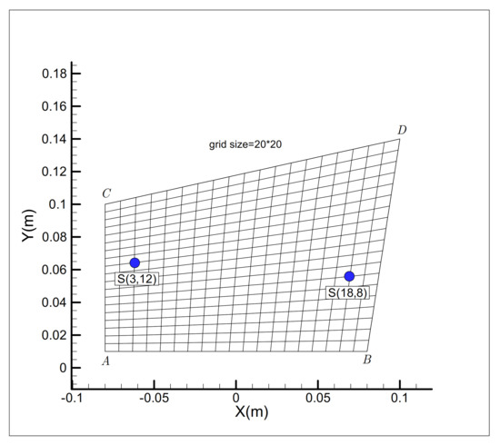
Figure 2.
Two different places for the single sensor , and , used to measure the temperature at time .
Before proceeding further, the accuracy and correct implementation of direct heat conduction solver should be confirmed. In order to validate the results from the direct problem solution, the temperature distribution for the heat conducting body used in this study is compared to the temperature distribution obtained from the commercial finite element software COMSOL. To do so, the timewise varying heat flux is considered. The temperature distribution obtained by the explicit solver, Equation (17), using the problem data given in Table 1, a grid size of , and the time step is shown in Figure 3a and the temperature distribution obtained by the finite element software COMSOL is depicted in Figure 3b. The temperature histories at the sensor places (Figure 4a) and (Figure 5a) obtained by both the explicit solver and the software COMSOL are compared and presented in Figure 4b or Figure 5b, respectively. Moreover, the temperature distribution at the final time at a given line, here along the nodes , , (Figure 6a) obtained by the explicit solver and the software COMSOL is shown in Figure 6b. The comparison between the results shows a very good agreement, thereby confirming the correct implementation of the explicit solver.
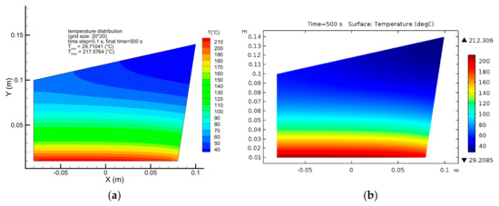
Figure 3.
Validation of the direct problem solver using the finite element software COMSOL. The result obtained by using our explicit code (a) and the result obtained by using COMSOL (b).
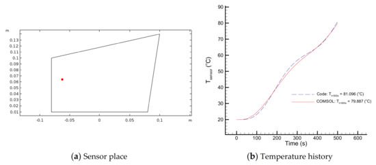
Figure 4.
Comparison of temperature history at the sensor place, , obtained from the explicit solver and the finite-element software COMSOL.
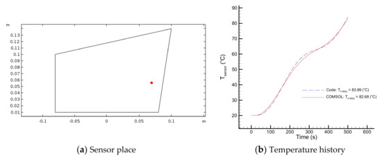
Figure 5.
Comparison of temperature history at the sensor place,, obtained from the explicit solver and the finite-element software COMSOL.
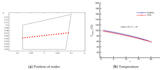
Figure 6.
Comparison of temperature at nodes , ; at the final time obtained from the explicit solver and the finite-element software COMSOL. The position of nodes (a) and the temperature comparison (b).
Two different places are considered for the single sensor to study the effect of the sensor location on the final results. The sensor is placed at the grid nodes and successively. Once the nodal temperature at the sensor place is calculated at each time , the sensitivity coefficients can be immediately computed during the transient solution using the explicit expressions obtained previously. This implies that the proposed sensitivity analysis scheme is very efficient and does not contribute significantly to the computational cost of the solution. As stated previously, we assume that is known when estimating , and vice versa. Initially we assume that the thermal conductivity is known and is equal to . The aim of inverse problem is now to recover the initially used specific heat using two different initial guesses:
These different initial guesses are selected so that they can reflect the accuracy and efficiency of the inverse analysis. The results of the recovery of the specific heat components and as well as the history of the objective function during the minimization process are shown in Figure 7 (for the initial guess ) and Figure 8 (for the initial guess ) by using the sensor placed at the node and Figure 9 (for the initial guess ) and Figure 10 (for the initial guess ) by using the sensor placed at the node and Figure 11 (for the initial guess ) by using the sensor placed at the node and the measurement error of . As shown in Table 2, without the measurement error, a 100% reduction in the objective function value and complete recovery of the unknown specific heat components are achieved by initiating the minimization process from both initial guesses, which shows the accuracy of the proposed sensitivity analysis scheme. Moreover, it can be seen that the proposed inverse analysis is not strongly affected by the errors involved in the temperature measurements, and the unknown parameters are recovered accurately.
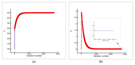
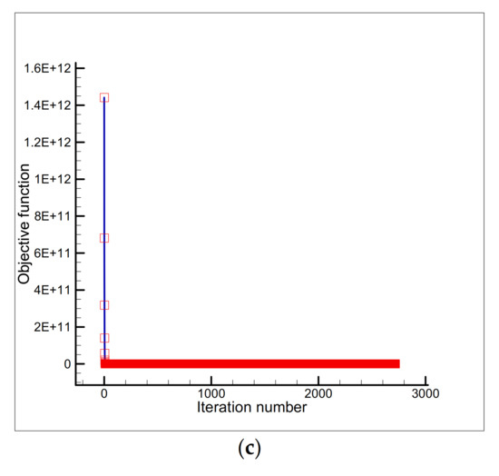
Figure 7.
Estimation of (a) and (b), and the objective function versus iteration number (c) using the initial guess and a single sensor placed at the node .
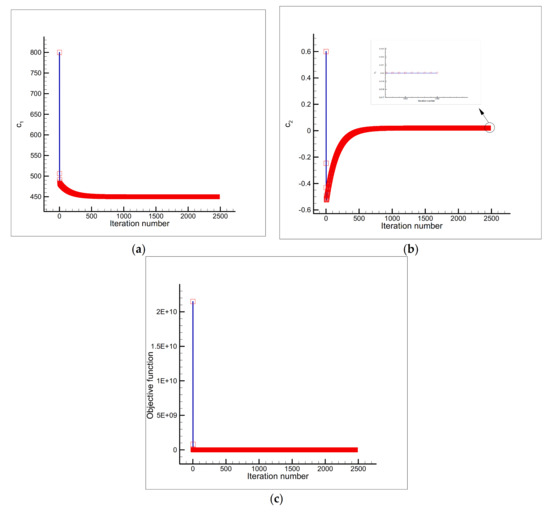
Figure 8.
Estimation of (a) and (b), and the objective function versus iteration number (c) using the initial guess and a single sensor placed at the node .
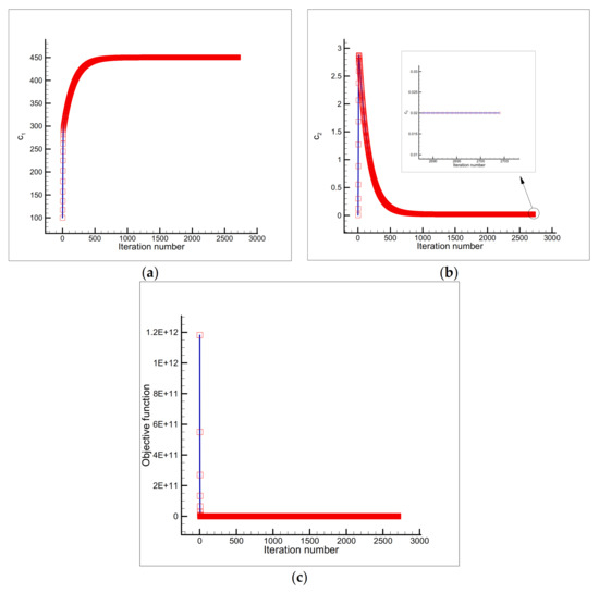
Figure 9.
Estimation of (a) and (b), and the objective function versus iteration number (c) using the initial guess and a single sensor placed at the node .
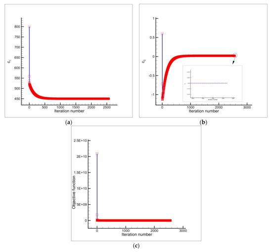
Figure 10.
Estimation of (a) and (b), and the objective function versus iteration number (c) using the initial guess and a single sensor placed at the node .
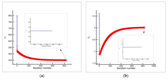
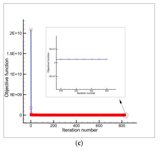
Figure 11.
Estimation of (a) and (b), and the objective function versus iteration number (c) using the initial guess and a single sensor placed at the node by considering the measurement error of ).

Table 2.
A summary of results for the estimation of the temperature-dependent specific heat components and ().
Then we assume that the specific heat is known and is equal to . The aim of inverse problem is then to recover the initially used thermal conductivity using two different initial guesses:
The results of the recovery of the thermal conductivity components and as well as the history of the objective function during the minimization process are shown in Figure 12 (for the initial guess ) and Figure 13 (for the initial guess ) by using the sensor placed at the node and Figure 14 (for the initial guess ) and Figure 15 (for the initial guess ) by using the sensor placed at the node and Figure 16 (for the initial guess ) by using the sensor placed at the node and the measurement error of . The summary of the results given in Table 3 reveals that without the measurement error a 100% reduction in the objective function value is obtained and the unknown thermal conductivity components are recovered accurately by initiating the minimization process from both initial guesses, which again shows the accuracy of the proposed sensitivity analysis scheme. Like the specific heat estimation case, it can be seen that the estimation of thermal conductivity components is not strongly affected by the errors involved in the temperature measurements and the unknown parameters are recovered accurately.
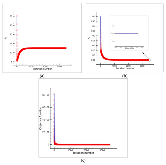
Figure 12.
Estimation of (a) and (b), and the objective function versus iteration number (c) using the initial guess and a single sensor placed at the node .
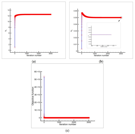
Figure 13.
Estimation of (a) and (b), and the objective function versus iteration number (c) using the initial guess and a single sensor placed at the node .
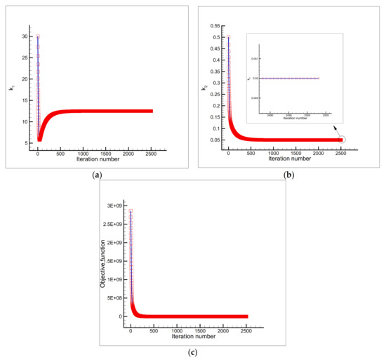
Figure 14.
Estimation of (a) and (b), and the objective function versus iteration number (c) using the initial guess and a single sensor placed at the node .
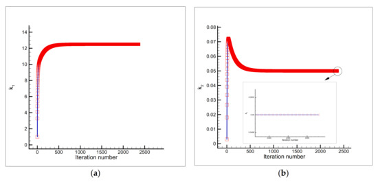
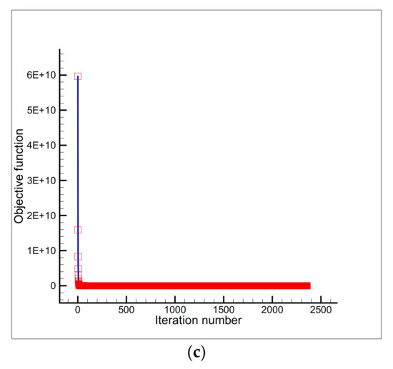
Figure 15.
Estimation of (a) and (b), and the objective function versus iteration number (c) using the initial guess and a single sensor placed at the node .
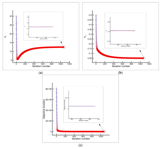
Figure 16.
Estimation of (a) and (b), and the objective function versus iteration number (c) using the initial guess and a single sensor placed at the node by considering the measurement error of ).

Table 3.
A summary of results for the estimation of the temperature-dependent thermal conductivity components and ().
5. Conclusions
Novel explicit expressions were derived for the sensitivity coefficients to estimate the temperature-dependent thermal conductivity and the temperature-dependent specific heat in general two-dimensional heat-conducting bodies using an inverse transient heat conduction analysis. Due to inability of the traditional finite-difference method to effectively handle the solution of heat transfer problems involving the irregular shapes, the irregular heat-conducting body was transformed into a regular computational domain to perform all computations related to the direct and inverse transient heat conduction solution using the finite-difference method, a method chosen for its widespread use in numerical heat transfer and ease of implementation. The irregular body was meshed using the elliptic grid generation technique because of its capability of producing a smooth grid over the body. Then, the governing equation and the associated boundary conditions were solved in the computational domain to obtain the temperature distribution over the body at each time step. In the inverse analysis, an objective function was defined based on the least squares norm and the explicit expressions were obtained for the sensitivity coefficients by differentiating the obtained expression for the temperature at the sensor location with respect to the unknown parameters. In addition to being accurate expressions, the use of explicit sensitivity coefficients eliminates the need for extra solution of direct problem to calculate the sensitivity coefficients using the finite-difference method or eliminates the need for solving adjoint problem to compute the gradient of the objective function with respect to the unknown parameters. We showed that, using the derived explicit sensitivity coefficients, the sensitivity matrix was computed in only one direct problem solution (at each iteration) and hence the computational cost was decreased significantly. The conjugate gradient method, as an iterative gradient-based optimization method, was used to minimize the objective function and reach the solution. A test case with different initial guesses and the sensor locations was presented to investigate the proposed inverse analysis. The obtained accurate results showed that the estimation of the temperature-dependent thermal conductivity or specific heat using the proposed method is not affected by the initial guess or sensor placement. Likewise, the results revealed that the method is not affected significantly by the error in the temperature measurement. This confirms that the proposed inverse analysis is very accurate, robust, and efficient.
Funding
This research was supported by funding from the European Union’s Horizon 2020 research and innovation programme under the Marie Skłodowska-Curie grant agreement No 663830.
Conflicts of Interest
The author declares no conflict of interest.
References
- Sawaf, B.; Ozisik, M.N.; Jarny, Y. An inverse analysis to estimate linearly temperature dependent thermal conductivity components and heat capacity of an orthotropic medium. Int. J. Heat Mass Transf. 1995, 38, 3005–3010. [Google Scholar] [CrossRef]
- Flach, G.P.; Özişik, M.N. Inverse heat conduction problem of simultaneousy estimating spatially varying thermal conductivity and heat capacity per unit volume. Numer. Heat Transf. Part A: Appl. 1989, 16, 249–266. [Google Scholar] [CrossRef]
- Talukdar, P.; Das, A.; Alagirusamy, R. Simultaneous estimation of thermal conductivity and specific heat of thermal protective fabrics using experimental data of high heat flux exposure. Appl. Therm. Eng. 2016, 107, 785–796. [Google Scholar] [CrossRef]
- Mohebbi, F.; Sellier, M.; Rabczuk, T. Estimation of linearly temperature-dependent thermal conductivity using an inverse analysis. Int. J. Therm. Sci. 2017, 117, 68–76. [Google Scholar] [CrossRef]
- Liu, F.B. A hybrid method for the inverse heat transfer of estimating fluid thermal conductivity and heat capacity. Int. J. Therm. Sci. 2011, 50, 718–724. [Google Scholar] [CrossRef]
- Czél, B.; Woodbury, K.A.; Gróf, G. Simultaneous estimation of temperature-dependent volumetric heat capacity and thermal conductivity functions via neural networks, International. J. Heat Mass Transf. 2014, 68, 1–13. [Google Scholar] [CrossRef]
- Özisik, M.; Orlande, H. Inverse Heat Transfer: Fundamentals and Applications; Taylor & Francis: New York, NY, USA, 2000. [Google Scholar]
- Alifanov, O.M. Inverse Heat Transfer Problems; Springer: Berlin/Heidelberg, Germany, 1994. [Google Scholar]
- Mohebbi, F. Optimal Shape Design Based on Body-fitted Grid Generation; University of Canterbury: Catembury, UK, 2014. [Google Scholar]
- Özişik, M.N.; Orlande, H.R.B.; Colaço, M.J.; Cotta, R.M. Finite Difference Methods in Heat Transfer; CRC Press: Boka Raton, FL, USA, 2017. [Google Scholar]
- Mohebbi, F. Function estimation in inverse heat transfer problems based on parameter estimation approach. Energies 2020, 13, 4410. [Google Scholar] [CrossRef]
- Polak, E.; Ribiere, G. Note sur la convergence de méthodes de directions conjuguées, Revue Française d’Informatique et de Recherche. Opérationnelle 1969, 16, 35–43. [Google Scholar] [CrossRef]
Publisher’s Note: MDPI stays neutral with regard to jurisdictional claims in published maps and institutional affiliations. |
© 2020 by the author. Licensee MDPI, Basel, Switzerland. This article is an open access article distributed under the terms and conditions of the Creative Commons Attribution (CC BY) license (http://creativecommons.org/licenses/by/4.0/).