Abstract
In this work, Monte Carlo simulations of magnetic properties of thin films, including the influence of an external pressure, are presented. These simulations were developed using a Hamiltonian composed by terms that represent the exchange interaction, dipolar interaction, Zeeman effect, monocrystalline anisotropy, and pressure influence. The term that represents the pressure influence on the magnetic properties was included, since for many applications, magnetic materials are a part of a multiferroic material together with a piezoelectric or a ferroelectric compound. Initially, the model was developed using generic parameters, in order to probe its suitable performance; after that, parameters were adjusted for simulating thin films of La0.67Sr0.33MnO3, a manganite with several technological applications because its Curie temperature is greater than room temperature. Including the pressure influence, it was observed the formation of several kind of FM/AF configurations as strip, labyrinth, and chess board forms. Furthermore, it was observed that, as the pressure increased, the critical temperature tended to decrease, and this result was in agreement with experimental reports.
1. Introduction
Lanthanum based manganites are compounds that attract great interest in the scientific community because of their highlighted properties [1]. For instance, doping this kind of material with a specific concentration of strontium generates a compound with several technological applications [2]. Among these compounds, La0.7Sr0.3MnO3 is the manganite that exhibits the highest Curie temperature (TC = 370 K) and is a very promising material for room-temperature applications [3,4,5]. In order to explore its potential applications, several techniques have been used to produce these materials [6,7,8]. Furthermore, there has been significant interest in modeling and simulating the magnetic properties of this material, especially using the Monte Carlo method [9,10,11,12], and the Metropolis algorithm, widely used in nanoelectronics and mechanics modeling problems [13].
Normally, simulated properties focuse on magnetic properties and consider the influence of exchange parameters, Zeeman effect, and the magneto-crystalline anisotropy [14,15]; however, these simulations do not consider changes in position due to external causes, such as an external pressure applied to a material. The influence of an external pressure on the final magnetic properties of a magnetic material is of great importance in applications for elastomers and allows one to adapt a built device to several geometries and uses. Moreover, these magnetic materials are normally combined with ferroelectrics and piezoelectrics, reaching multiferroic properties. In the case of piezoelectrics, the material is deformed, and the deformation produces an electric field; the deformation affects the piezoelectric material, and also the magnetic part of the system, changing its magnetic behavior [16].
In the present paper, we study the magnetic properties of magnetic thin films using a Hamiltonian composed of several terms including the influence of an external pressure. We focus on observing the antiferromagnetic regions distribution that forms special configurations. The work is developed using the Monte Carlo method combined with the Metropolis algorithm; we also analyze the effect of pressure on the critical temperature of a material.
The paper is organized as follows: The model of the superlattice is presented in Section 2, where we summarize the principal steps used in the calculation of the ground-state configurations of the system; in Section 3, we show the results of the configurations formed depending on the pressure parameter, and the critical temperature dependence on the pressure; and finally, we state concluding remarks in Section 4.
2. Materials and Methods
In this section the methodology for the construction of the model is defined. The geometry considerations for the simulated sample, the Hamiltonian used, and its different contributions are presented, for both cases, the generic and specific LSMO model.
2.1. Generic Model
The first step is the construction of a generic model for a magnetic layer which consists of a rectangular arrangement of L × L × d dimensions in the x, y, and z directions, respectively. The integer positions of this arrangement (i,j,k) represent the positions of the unit cells of the magnetic ions. Periodic boundary conditions are chosen in the directions of the xy plane and free boundary conditions in the z direction. Hence, the built structure becomes an infinitely extended surface in xy [13]. At first, in order to test the model, at each point of the magnetic lattice, a magnetic moment of magnitude 1 is assigned, with a random direction in the space (Heisenberg) [17] to simulate a state of high temperature (high magnetic disorder). For the magnetic system, the Hamiltonian is considered as described below:
where Hex, Hdip, Hf, and Han correspond to magnetic exchange, magnetic dipole interaction, Zeeman interaction, and magnetocrystalline anisotropy, respectively. The first term is calculated according to the following expression:
where J the integral magnetic exchange, is the magnetic moment associated with the site I, and the sum runs for j = 1, ⋯, 6 first neighbors. Some models suppose an exponential decay of the exchange interaction with the distance between magnetic moments by means of an expression of the form:
The decreasing tendency was taken according to reports in the literature for this manganite [18]. J0 and a are the exchange constant and the lattice parameter to zero stress, respectively, rij is the distance between the magnetic site i and its neighbor j, and λ is a characteristic length that depends on the material and accounts for the magnitude of J variations depending on the stress. In this case, the characteristic length refers to the distance at which the pressure induces stress and affects the magnetic exchange [19]. The d dependence of J for values lower than 5a can be considered with an exponential tendency, which is consistent with the well-known result of the disorder mediated RKKY interaction. A rapid decay of J for d greater than 6a, due to the oscillatory behavior of the RKKY interaction, encourages us to neglect the exchange interaction at higher distances and consider a cut-off radius lower than this value [20].
When the sample is subjected to a compressive strain in the z direction, there are two ferromagnetic contributions to the exchange J, one in the plane (Jx = Jy) and another perpendicular to the plane of the sample (Jz),
where and the exchange interaction has been rewritten in terms of the relative pressure P, Young’s modulus, Y, and the Poisson coefficient, ∊. Studies of first principles have reported the differentiated appearance of these two contributions and changes in the critical temperature with deformation, which can reach several tens of degrees [21]. For uniaxial pressure (P) in the z direction, these distances are calculated in terms of the Young’s modulus (Y) and the Poisson coefficient (∊) of the material; then, rij, is represented by Equation (5):
where rijx, rijy, rijz are the distances in x, y, and z between the magnetic site i and the magnetic site j, once pressure is applied. In addition, rijox, rijoy, and rijoz are the distances between the magnetic site i and the magnetic site j to zero deformation. In the case of a simple cubic cell, rijox = rijoy = rijoz = a; then, replacing Equation (5) in Equation (3), we obtained Equation (4).
The contribution to Hamiltonian, that it is due to dipolar interaction [19], is given by:
where for each position i of the magnetic sample, the sum runs over all the neighbors within a radius RC = 6a. The parameter g, is the magnitude of dipolar interaction between all the pairs of spins Si and Sj. The dipolar parameter strongly depends on the material, since it is inversely proportional to the interatomic distance [22]. The calculation of this interaction, even for a cutoff radius of a few lattice parameters, has a high computational cost and the convergence of the series is slow. For this work, a mixed method has been used that includes the choice of a cutoff radius for the one-to-one interaction with the neighbors of the magnetic site, and a method of the fast multipole, for more distant neighbors, which consists of the partition of the sample in boxes or subregions of the system, for which, an effective magnetic moment is calculated. For these more distant neighbors, the dipolar interaction is calculated between the magnetic site and each of the boxes, as if it were a single magnetic neighbor. In this way, it is possible to extend the range of the dipolar interaction to hundreds of cell units. Studies carried out on low dimension systems have succeeded in reproducing relevant characteristics of magnetic structures using small cutting radius [23,24].
In this work, the variation of the dipolar interaction term due to the pressure is taken into account when calculating the distances between the different magnetic sites (rij), since they are dependent on the deformations caused, according to Equation (5).
Finally, the field terms of Zeeman contribution and uniaxial anisotropy in the x-direction are given by [25]:
where h is the magnetic field, K the anisotropy constant, is the component in x of the magnetic moment Si and the sums sweep every site in the sample. Similarly, uniaxial anisotropies can be defined in the y and z directions.
Magnetization of the magnetic layer per unit cell and magnetic susceptibility are used to study the magnetic behavior of the sample, in addition to critical temperatures and magnetic hysteresis cycles. The average magnetization in equilibrium ⟨|m|⟩ on all the states of the system and susceptibility are obtained by:
where
The index i indicates each of the Monte Carlo steps when performing a complete scan of the magnetic sample; the index j represents each of the atoms of the magnetic cell; MCSmax is the maximum number of Monte Carlo steps; and N0 indicates the number of steps, from which the averages in the equilibrium are obtained for the calculation of the observables.
After randomly assigning the magnetic moments to each sample site, the sample is again scanned by proposing random changes in the magnetization of the site at a given temperature. This change is accepted or rejected according to the Metropolis algorithm associated with the Monte Carlo method [9]. The network was visited 15,000 times (Monte Carlo steps) to ensure convergence in the calculation of observables; and the average of the observables was calculated in the last 5000 mcs. This procedure was repeated for each temperature within the range of 5–800 K with a delta temperature of 5 K. This generic model served to simulate the effect of the magnetic dipole interaction on the magnetization of the sample and to consider the size effects, pressure, and magnetic field.
2.2. LSMO Model
After considering the generic model, we proceeded to adjust its parameters to model the behavior of a film . For this level of doping, a simple cubic structure (spatial group Pnma) typical of perovskites is reported [26] in accordance with the type of sample considered in the generic model. For the above, a more realistic spin value was used. At each point of the magnetic sample, it was assigned a magnetic moment of magnitude equal to the average moment per unit cell, corresponding to that expected for this compound , for , where is the Bohr magneton. This way for calculating the average magnetic moment in compounds with mixed spin values has been previously reported [27].
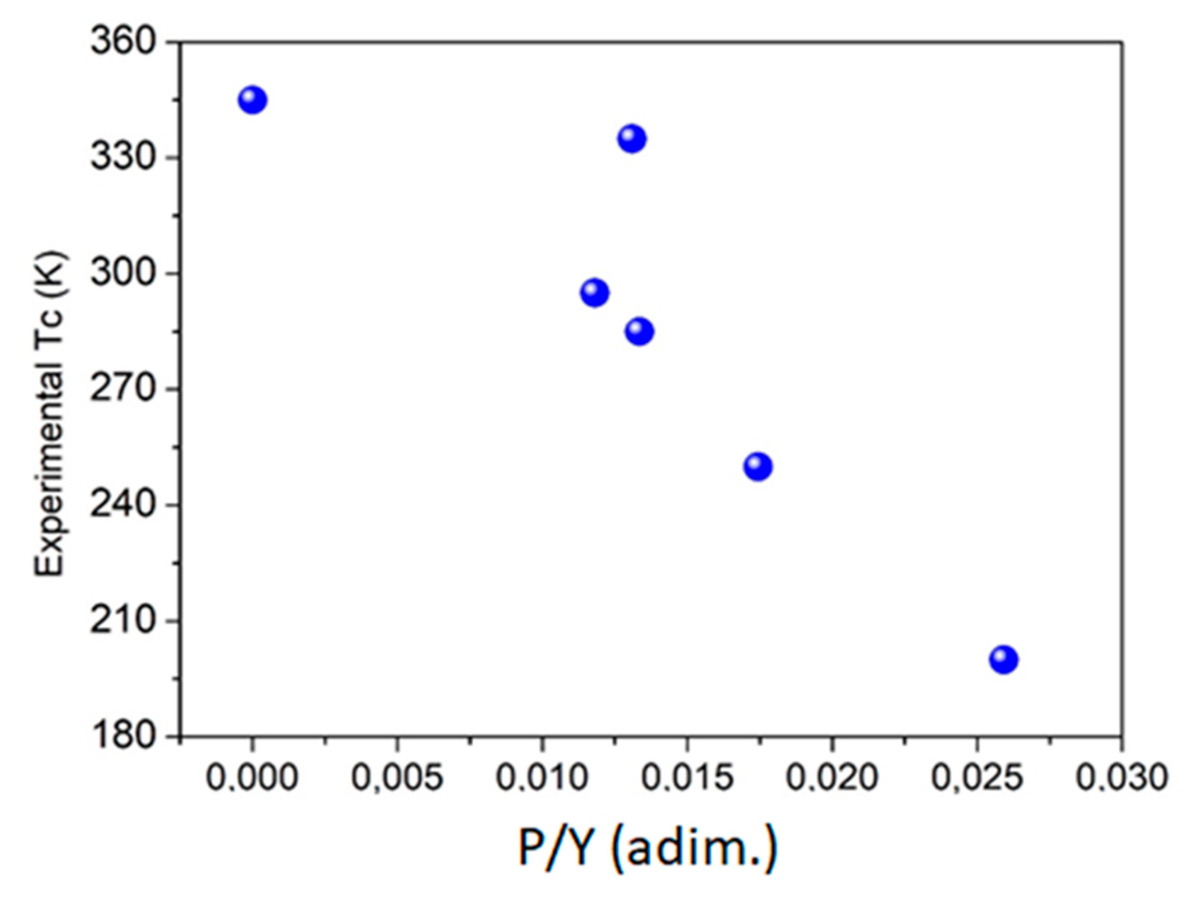
The LSMO is within the compounds with strongly correlated electrons [21] and, as expected, according to the values of its Young’s modulus and Poisson coefficient, there is an increase in the magnetic interaction and its critical temperature because of the compressive increase in the z direction of the film. This situation does not occur experimentally; on the contrary, by increasing compression in this direction, the net magnetic interaction with first neighbors decreases, and thus the critical temperature of the material. When LSMO films are grown on different substrates, the degree of coherence between the materials in contact induces tensions in the interface which affect the magnetic behavior and the critical temperature of the magnetic system. Figure 1 shows some of these experimental results, in which it is observed how the critical temperature decays approximately linearly when a compressive stress on the film decreases its dimensions in the perpendicular direction, (each deformation corresponds to the generated one by the difference between the lattice parameter of the manganite and the substrate used) [28]. It is remarkable the reduction of the critical temperature in these reports, which reaches up to ∆Tc ≈ 43%.
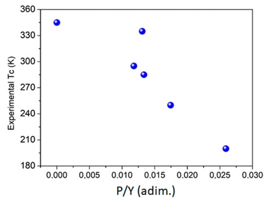
Figure 1.
Experimental critical temperature values of La2/3Sr1/3 MnO3 films at different deformations [23].
Bearing in mind the above, it is assumed that the magnitude of the exchange interaction obeys a law of exponential decay with the deformation of the structure P/Y, along the z-axis,
where J0 is the value of the exchange constant at zero deformation, J is the value of the average exchange constant to first neighbors, and ω is a parameter whose value is linked to the magnitude of the changes in the critical temperature.
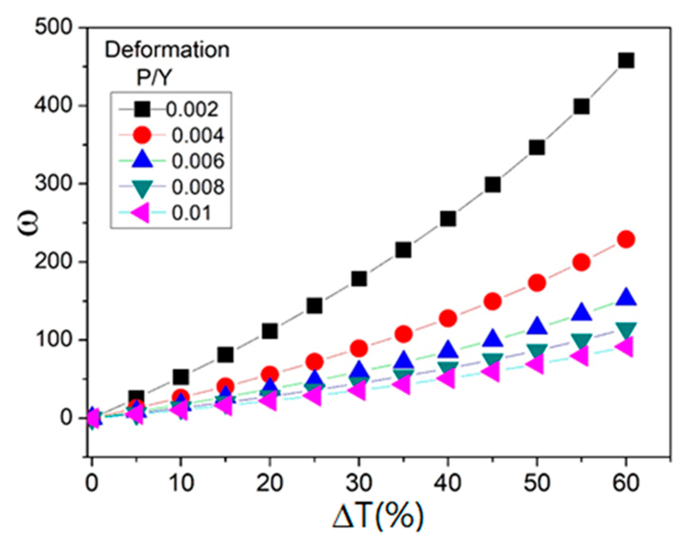
Figure 2 shows the relationship between the parameter ω, in terms of the percentage change in the simulated critical temperature to different values of deformation. Once the value of the exchange J is identified, which reproduces the critical temperature of the material at zero deformation, it is possible to approximately calculate the percentage changes in ∆Tc, which occur at different deformations for different values of ω.
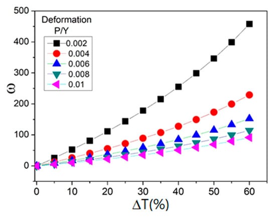
Figure 2.
Parameter ω vs. percentage change in the critical temperature for several deformation values.
According to the experimental values reported in Figure 1, a deformation of the sample of P/Y = 0.01 causes a ∆Tc ≈ 15%; for these temperature changes and deformation value, it is obtained ω ≈ 16.7 in the corresponding curve (Figure 2). It should be noted that experimental data is used to reproduce trends in the material, without forgetting that other reports may differ a little, given the sensitivity of the critical temperature of this compound to variables such as type and quality of the substrate, growth method, quality of the film obtained, thickness, time, among others.
3. Results and Discussion
Results of the proposed model considering the influence of pressure on the formation of ferromagnetic/antiferromagnetic (FM/AF) configurations in LSMO films are presented. First, the effects of the dipolar interaction on a generic magnetic layer are considered ( taking into account uniaxial pressure. Second, some magnetic configurations are identified in the equilibrium at low temperature. Finally, the parameters of the generic system are adjusted for the description of a particular system, in this case an LSMO structure .
3.1. Effect of the Dipolar Interaction on the Magnetization for the Generic Model
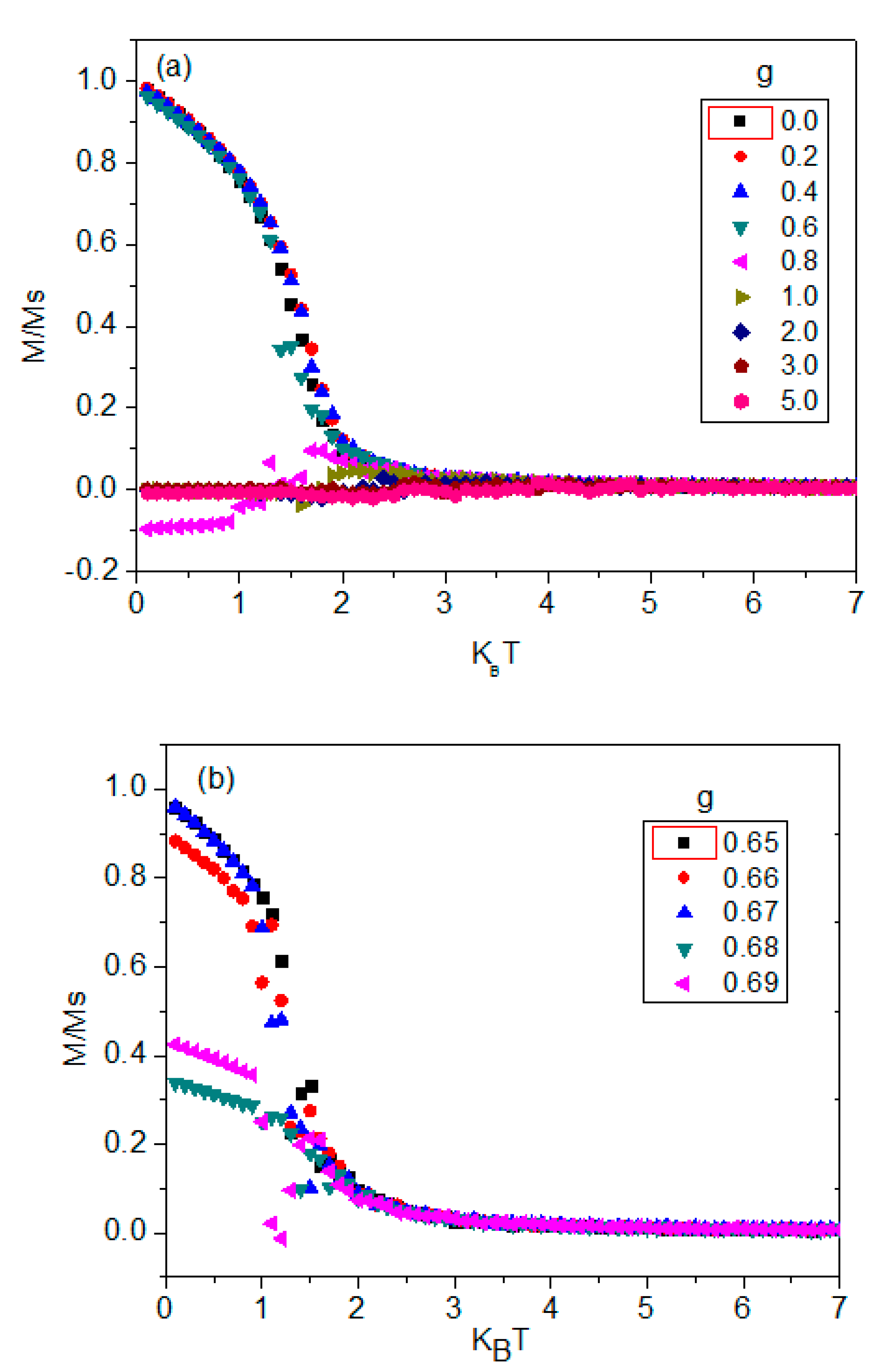
Figure 3a shows the simulated magnetization vs. temperature curves at different values of g, in a layer with thickness, d = 5 unit cells, and with a P/Y = 0.002. It was observed that, for g > 0.69, there was an abrupt fall in the magnetization; therefore, simulations were carried out between 0.65 ≤ g ≤ 0.69. In this range, it was observed that the FM ordering rapidly decreases. This effect does not correspond to a fall of magnetization due to magnetic disorder in the spins, or the transition to the paramagnetic state; this effect is caused by the formation of AF configurations in the sample, as presented below. Normally, the dipolar interaction between two spins tends to be lower than the exchange interaction; then, the dipolar interaction gains real importance in the case of the interaction between two regions of magnetic domain, as they calculated by means of the fast dipole method, because these regions contain hundreds or thousands of individual spins. The antiferromagnetic region formation, because of the increase in the dipolar interaction, has been previously shown [29]. Furthermore, in three dimensions, the lowest energy state of a collection of dipoles can be ferromagnetic in structures with a high coordination number, such as face centered cubic and hexagonal closest packed, whereas it can be antiferromagnetic in a simple cubic lattice, or zinc blend, where the coordination number is low.
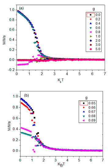
Figure 3.
(a) Normalized magnetization curves vs. temperature at different values of the dipolar interaction parameter g, in a magnetic layer with thickness, d = 5 unit cells; (b) Magnetization curves vs. temperature at the interval where the ferromagnetic order decays. Curves were obtained at P/Y = 0.002.
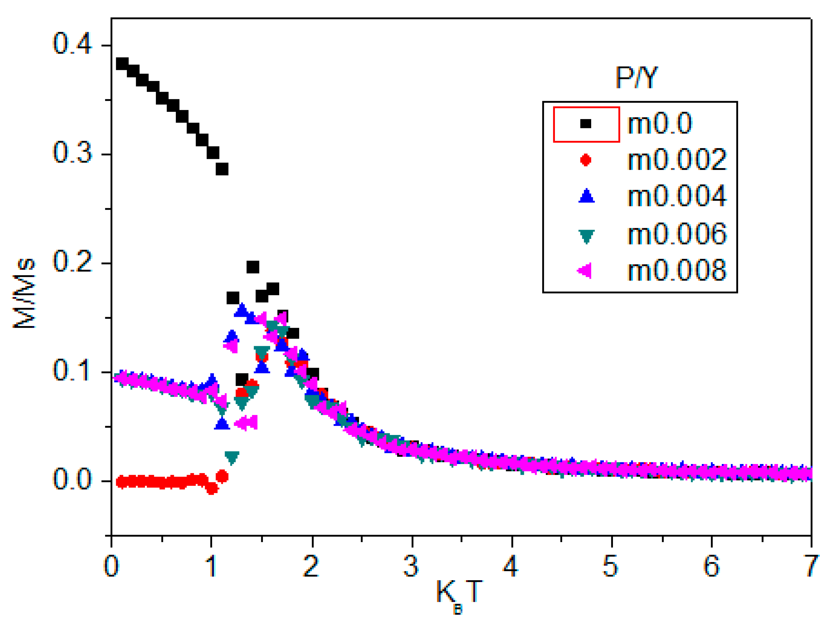
Figure 4 shows the behavior of the magnetization with the temperature at different pressure values (P/Y), for the case g = 0.69. It is observed, as for this value, the system is especially sensitive to changes in pressure. At zero pressure, the sample already exhibits the effects of the dipolar interaction, manifesting a maximum magnetization of 40% with respect to the total possible magnetization in the x direction. As the pressure increases, the magnetization in this direction decays significantly. It should be noted that with values of g less than 0.67, the system behaves like a pure ferromagnet, similar to the LSMO.
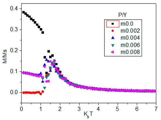
Figure 4.
Effect of pressure on the magnetization curve vs. temperature for a value g = 0.69.
In order to determine the influence of the dipolar interaction, and to analyze the relative weight of the different contributions to the proposed Hamiltonian and its effect on the magnetic configurations of the system, the following ratios among the constants were considered for the simulations of the present work:
In the simulations, a wide range was swept for these parameters, i.e., and . These intervals take into account scenarios for samples with weak exchange interactions (strong dipolar interaction) or strong exchange interactions (weak dipolar interaction), as well as the case in which the magnitude of both interactions are comparable.
3.2. Magnetic Configurations
Initially, we analyze the influence of the dipolar interaction, on the magnetic configuration of the sample. Figure 5 shows the orientation of the magnetic moments for samples with constant g = 0.66, g = 0.69 and g = 1.0, in which a uniaxial anisotropy is considered to be in the planar direction x. In this representation, the black color is assigned to the spins with a preferred orientation towards the axis +x, and the red color is assigned to the spins with a preferred orientation towards the axis −x. For g = 0.66, the system at a low temperature and zero pressure shows a FM magnetic array, with a fringe in the −x direction. This strip is the beginning of the AF ordering that arises at higher pressures. For g = 0.69, the sample without pressure has two regions, one preferably FM and another with AF arrangement in the form of stripes. Previous theoretical and experimental studies have reported the appearance of magnetic configurations in geometric forms (textures), in the fundamental state of magnetic systems, for which the dipolar interaction plays an important role. For example, configurations of magnetic domains in the form of a chessboard, stripes along the field direction, or labyrinths structures have been reported [30,31].
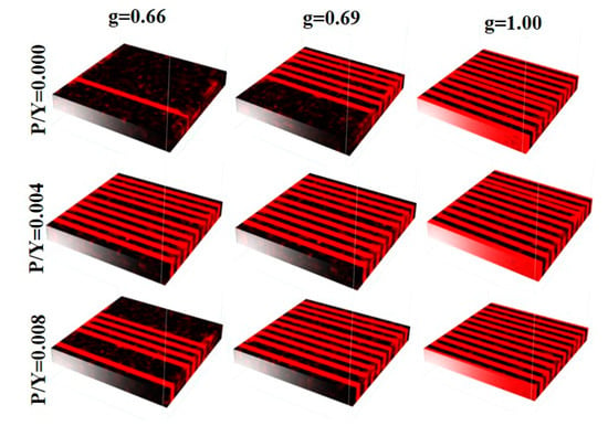
Figure 5.
Magnetic configurations. Red indicates magnetic alignments of stripes in the −x direction and black indicates alignments in the +x direction.
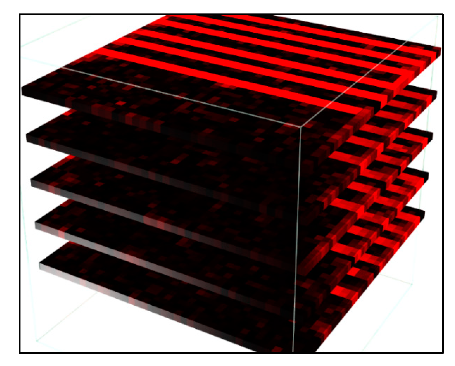
Again, the increase in pressure leads to an AF configuration for the total sample. Finally, for g = 1.0, the dipolar interaction is strong enough to ensure the AF arrangement even at zero pressure. A detail by layers of the sample (Figure 6), for the case g = 0.69 and P/Y = 0.0, allows us to identify that the array of stripes is AF in planes parallel to the xy plane, and FM between those planes.
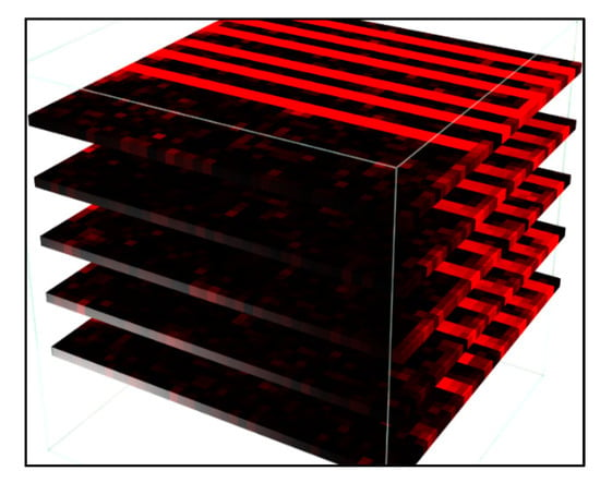
Figure 6.
Layered view of the magnetic sample corresponding to g = 0.69 and P/Y = 0. Red indicates magnetic alignments of stripes in the −x direction (from left to right) and black indicates alignments in the +x direction (from right to left).
The previous behavior can be understood by remembering that the dipolar interaction is a long-range collaborative phenomenon between each magnetic site with the rest of the sample, whose intensity is linked to the distance between the network sites. This distance, in turn, depends on the magnitude of the pressure applied (perpendicular to the sample) and the elastic constants of the material (Young’s modulus and Poisson coefficient). As previously mentioned, dipolar interaction tends to align antiparallel pairs of neighboring magnetic sites. The above, together with the uniaxial anisotropy considered on the x, y, and the acting field in the +x generate the conditions for the appearance of the AF stripped-like structure linked to lower magnetization states. It is worth noting the existence of such behaviors, which, in theory, establish the possibility of modulating the magnitude of the magnetization and also the nature of the magnetic configurations through pressure or deformations of the material.
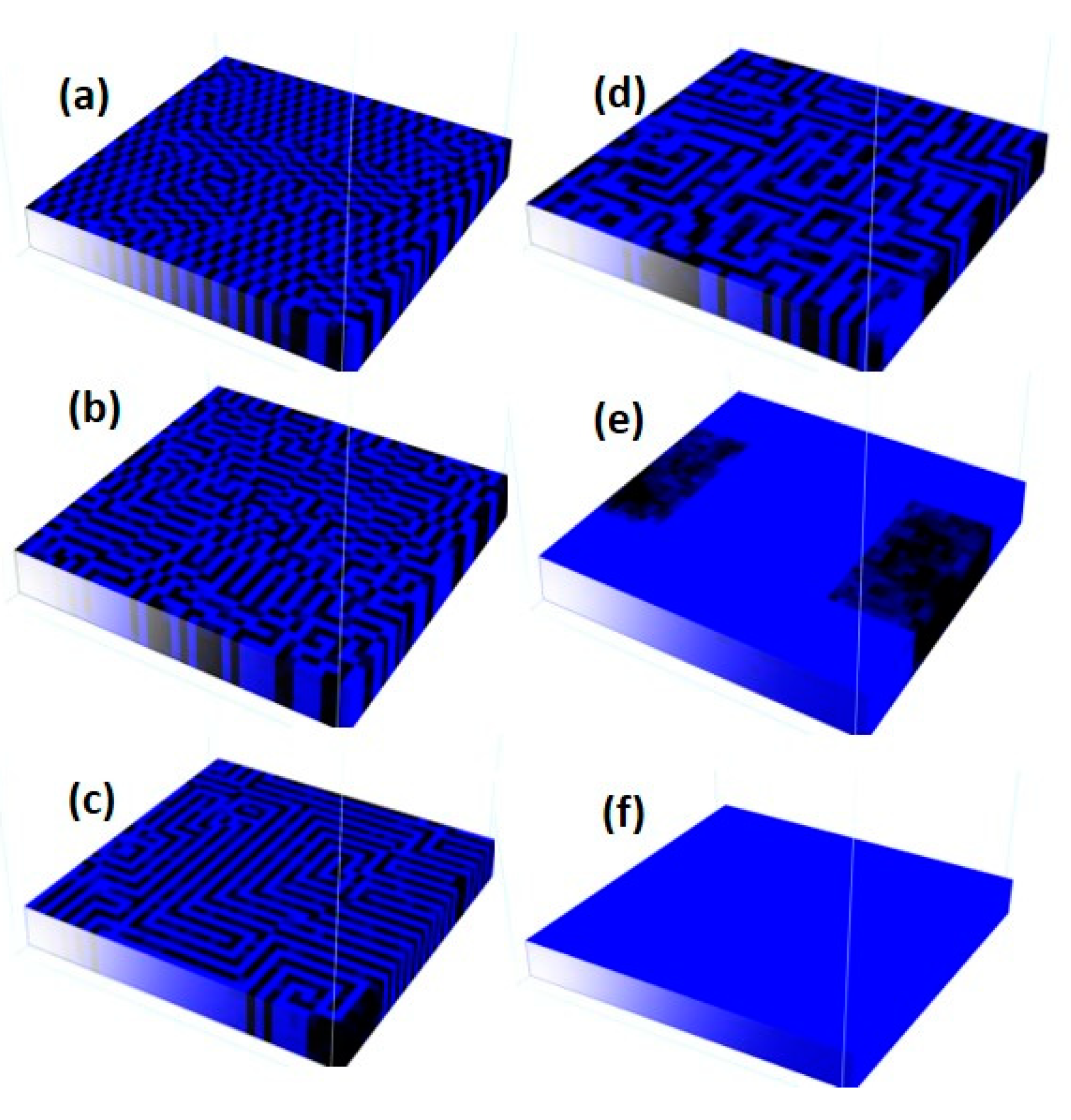
Figure 7 exhibits different patterns in the formation of magnetic domains as a function of the parameters , y, and , considering a uniaxial anisotropy perpendicular to the sample. The black color indicates polarization in the +z direction (out of plane), and the blue color indicates polarization in the −z direction (entering the plane).
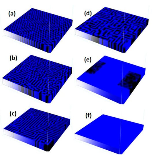
Figure 7.
Evolution characteristic of magnetic configurations. Blue indicates magnetic alignments in the −x direction and black indicates alignments in the +x direction. Column: . (a) ; (b) ; (c) ; (d) ; (e) ; (f) .
With respect to the system with values of = 0.3 and = 0.1 (Figure 7a), the dipolar interaction is dominant, and the system stabilizes for AF-type chessboard arrangements in the xy plane (Ising type behavior with alignment in ±z). The rise of results in the disappearance of the previous configuration and, subsequently, to the combination of minimum energy states, corresponding to the short- and long-range interactions. This generates AF arrays of labyrinth stripes of increasing thickness (Figure 7b–d) ending with an FM interaction between planes (Figure 7e,f).
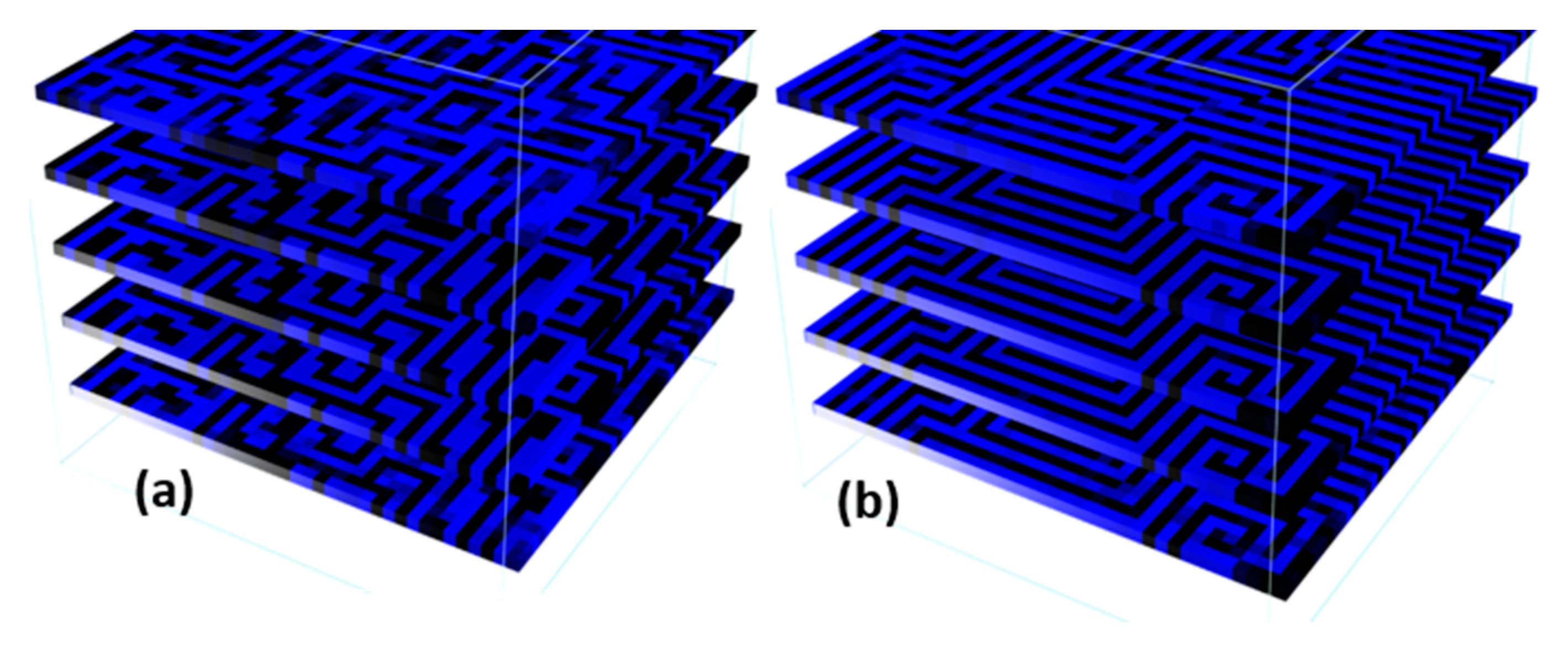
Figure 8 shows patterns of magnetic domains in the form of labyrinths for and values of and = 1.0. It can be seen how the definition of the domains is AF in each plane and FM between planes, with a greater definition of the labyrinthine domains for 1.0; while for 0.5, the patterns still present some lags of the chessboard-like configuration typical of the lower values of .

Figure 8.
Layered detail (a) = 0.3, = 0.5; (b) = 0.3, = 1.0. Blue indicates magnetic alignments in the −x direction and black indicates alignments in the +x direction.
The appearance of the previous patterns can be explained from the energetic contributions considered in the Hamiltonian and from the tendency of the system to stabilize in minimum energy configurations. First, the term, anisotropy K, establishes the preference of the magnetic moments to be aligned in a certain direction (in this case the z-axis). In addition, the exchange constant J is a measure of the intensity with which two neighboring magnetic moments tend to align in parallel. Finally, the constant g provides a measure of the intensity of the dipolar interaction between all the pairs of magnetic moments in the sample. This dipolar interaction forces nearby magnetic moments within the same plane xy to be aligned antiparallel [30].
Small values of ease the formation of domains in the plane. Furthermore, if is small, it dominates the dipolar interaction generating domains of pairs of antiparallel magnetic moments, which leads to a chessboard-like configuration. Once this configuration is established, an increase in the value of determines that the minimum energy is reached for configurations in the plane with a greater presence of FM domains in xy planes. In this way, the magnetic moments in the plane tend to the formation of fringes with magnetic moments aligned in parallel (FM), in a distribution that preserves an order (AF) between stripes. In the absence of a preferred direction for such stripes in the plane, the distribution of domains take several presentations in the form of labyrinths. A subsequent increase in the value of the ratio favors the presence of FM configurations in the plane, which is given by the FM junction between the mentioned stripes making them thicker. To this respect, the labyrinthine distribution gradually disappears, until reaching a certain value of , a completely FM arrangement of the sample in the direction of anisotropy.
In conclusion, the Hamiltonian and the Monte Carlo Method used in this work allowed us to reproduce magnetic configurations that have been reported in other studies [31,32,33,34,35,36].
3.3. Effect of the Dipolar Interaction on the Magnetization for the LSMO Model
According to the behavior analyzed for the generic layer, it is concluded that the contribution of the dipolar interaction must not be dominant (g < 0.67) to obtain behaviors in agreement with those observed in the ferromagnetic compound LSMO. The theory of finite scaling [37] predicts the effect of size on magnetic behavior in systems L × L × d equivalent to those treated here. It is reported how the critical temperature increases with the number of monolayers. When comparing with the limit values, an overlap of the two-dimensional (2D) and three-dimensional (3D) dimensionalities is observed, in which, depending on the thickness, the system can be characterized by a fractional dimension between two and three. For thicknesses above eight monolayers, the universality of the system resembles more than that of a 3D system; while below this value the dimensionality rapidly decreases [38,39]. Using this finite scaling theory, the exchange constant J0 was determined. The experimental critical temperature for LSMO in bulk (Tc ≈ 369 K) [40] was reproduced with a magnetic exchange constant of J0 = 22.05 mV.
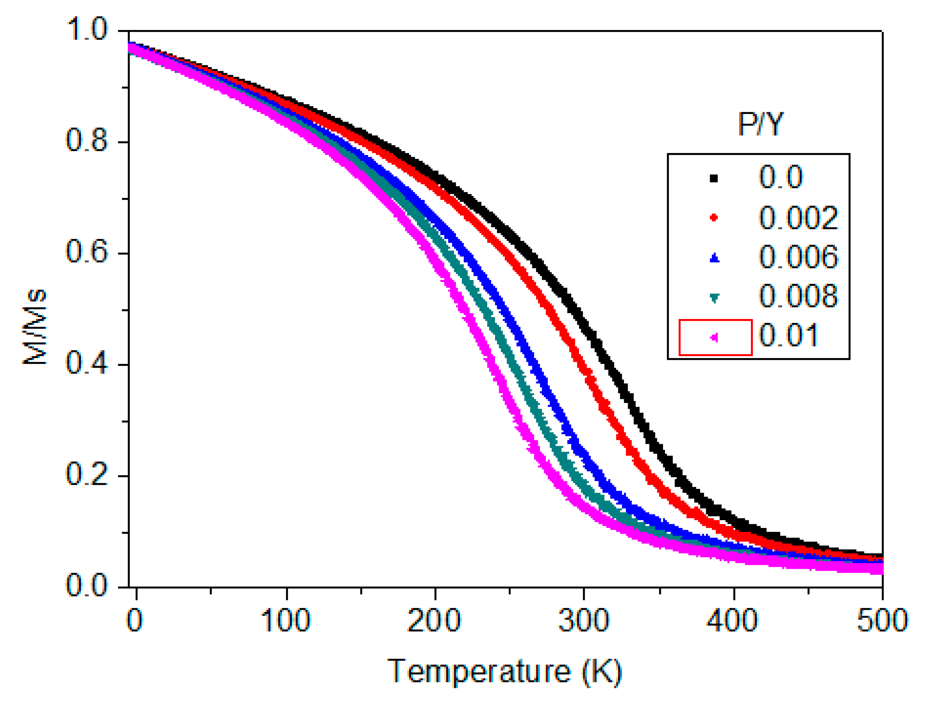
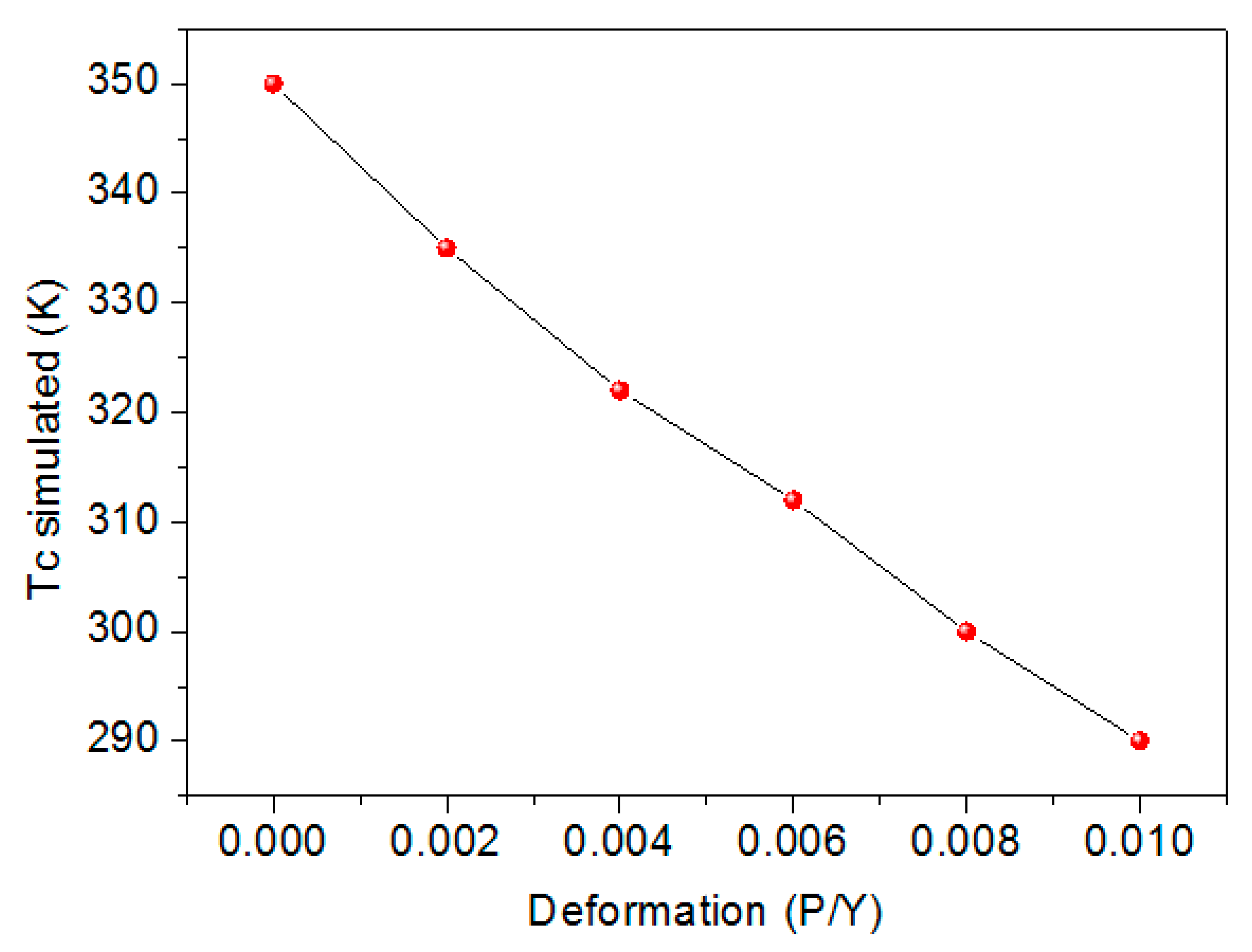
Figure 9 and Figure 10 show the curves of magnetization vs. temperature at different pressures, and temperature vs. deformation, respectively, using the parameter J0 = 22.05 meV. The results of the simulations show, as expected, a linear reduction of the critical temperature by applying a uniaxial stress in a direction perpendicular to the plane of the sample.

Figure 9.
Behavior of the magnetization of an LSMO film (d = 9 unit cells) at different levels of deformation.
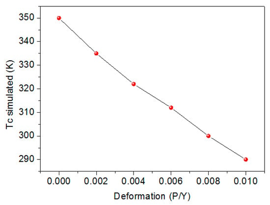
Figure 10.
Simulated critical temperature behavior of an LSMO film of thickness d = 9 with respect to deformation in the z direction.
Changes in the critical temperature of the LSMO in real samples can be explained from the energy contribution governed by the double exchange, which, in turn, depends on the distances between magnetic sites and the coordination number with their other nearby neighbors. The smaller the distance between magnetic sites, the greater the intensity of the ferromagnetic coupling, favoring a higher critical temperature. If the effort is uniaxial (perpendicular to the film), as proposed in this work, there are smaller distances between magnetic ions in this direction and, greater in the planar direction, according to the magnitude of the Young’s modulus and the Poisson coefficient. This implies that deformations in the z-axis, favor an increase in critical temperature and deformations in the xy plane favor a decrease in this temperature. The behavior observed in the experimental reports of the critical temperature of the LSMO at different levels of deformation (Figure 1) coincides with that theoretically obtained by simulations for this same compound.
4. Conclusions
A generic model for studying the behavior of a thin magnetic layer was constructed considering a Heisemberg Hamiltonian with exchange, dipolar, field, and anisotropy contributions. The aforementioned introducing elastic constants, such as the Young’s modulus and the Poisson coefficient, which allowed us to measure the effect of pressure on this layer. Variation of the Hamiltonian parameters allowed us to reproduce magnetic configurations, such as strip, labyrinth, and chess board forms which have been experimentally reported.
It was evidenced how variation of the magnetic dipolar interaction parameter g could generate FM or AF orderings, which translated into significant changes in the magnetization of the system. For an anisotropy in the x direction, the existence of a value 0.65 ≤ 𝑔 ≤ 0.69 was identified, from which the FM ordering in the x direction decreased drastically giving rise to AF orderings in the xy plane and, FM between planes in the form of parallel stripes in the x direction. For values of g in this range, the magnetic system was especially sensitive to changes in pressure. The possibility of modulating the magnitude of the magnetization and also the nature of the magnetic configurations through pressure or deformations of the material was established.
The simulations carried out on the system allowed us to demonstrate an approach between the proposed model and the experimental behavior of materials with cubic perovskite structure. In particular, it was possible to find Hamiltonian parameter values for LSMO films obtaining shifts in the critical temperature according to those reported experimentally for changes in the deformation of these structures.
Author Contributions
Conceptualization, H.H.O.-Á. and E.R.-P.; methodology, H.H.O.-Á., F.N.J.-G. and E.R.-P.; software, H.H.O.-Á.; validation, H.H.O.-Á., J.D.A.-G. and E.R.-P.; formal analysis, H.H.O.-Á., F.N.J.-G., J.D.A.-G. and E.R.-P.; investigation, H.H.O.-Á., F.N.J.-G., C.M.-N., J.D.A.-G. and E.R.-P.; resources, E.R.-P.; data curation, H.H.O.-Á.; writing—original draft preparation, H.H.O.-Á., F.N.J.-G., C.M.-N., J.D.A.-G. and E.R.-P.; writing—review and editing, H.H.O.-Á., F.N.J.-G. and E.R.-P.; visualization, H.H.O.-Á.; supervision, E.R.-P.; project administration, E.R.-P.; funding acquisition, E.R.-P. All authors have read and agreed to the published version of the manuscript.
Funding
This research received no external funding.
Acknowledgments
The authors want to thank the National University, the Autonomous University, and the University of Caldas for giving us the time and physical space to develop this research.
Conflicts of Interest
The authors declare no conflict of interest.
References
- Jiang, S.P. Development of lanthanum strontium manganite perovskite cathode materials of solid oxide fuel cells: A review. J. Mater. Sci. 2008, 43, 6799–6833. [Google Scholar] [CrossRef]
- Rasic, D.; Sachan, R.; Prater, J.; Narayan, J. Structure-property correlations in thermally processed epitaxial LSMO films. Acta Mater. 2019, 163, 189–198. [Google Scholar] [CrossRef]
- Ichikawa, H.; Nozawa, S.; Sato, T.; Tomita, A.; Ichiyanagi, K.; Chollet, M.; Guerin, L.; Dean, N.; Cavalleri, A.; Adachi, S.-I.; et al. Transient photoinduced ‘hidden’ phase in a manganite. Nat. Mater. 2011, 10, 101–105. [Google Scholar] [CrossRef] [PubMed]
- Zi, Z.; Fu, Y.; Liu, Q.; Dai, J.; Sun, Y. Enhanced low-field magnetoresistance in LSMO/SFO composite system. J. Magn. Magn. Mater. 2011, 324, 1117–1121. [Google Scholar] [CrossRef]
- Zi, Z.; Fu, Y.; Liu, Q.; Dai, J.; Sun, Y. Critical behavior of ensembles of superparamagnetic nanoparticles with dispersions of magnetic parameters. J. Phys. Condens. Matter 2019, 31, 375801. [Google Scholar] [CrossRef]
- Ghosh, A.; Sahu, A.K.; Gulnar, A.K.; Suri, A.K. Synthesis and characterization of lanthanum strontium manganite. Scr. Mater. 2005, 52, 1305–1309. [Google Scholar] [CrossRef]
- Yang, C.-K.; Yamazaki, Y.; Aydin, A.; Haile, S.M. Thermodynamic and kinetic assessments of strontium-doped lanthanum manganite perovskites for two-step thermochemical water splitting. J. Mater. Chem. A 2014, 2, 3065–3071. [Google Scholar] [CrossRef]
- Gupta, S.; Zhong, Y.; Mahapatra, M.; Singh, P. Processing and electrochemical performance of manganese-doped lanthanum-strontium chromite in oxidizing and reducing atmospheres. Int. J. Hydrog. Energy 2015, 40, 13479–13489. [Google Scholar] [CrossRef]
- Ortiz-Álvarez, H.H.; Bedoya-Hincapié, C.M.; Restrepo-Parra, E. Monte Carlo simulation of charge mediated magnetoelectricity in multiferroic bilayers. Phys. B Condens. Matter 2014, 454, 235–239. [Google Scholar] [CrossRef]
- Loudaini, A.; Aggour, M.; Mounkachi, O.; Bahmad, L. Electronic, magnetic properties and magnetocaloric effect in La 0.67 Sr 0.33 MnO 3 compound: Ab initio calculations and Monte Carlo simulation. Solid State Commun. 2019, 295, 5–11. [Google Scholar] [CrossRef]
- Ahmed, M.R. Monte Carlo study of the effect of charge ordering on the electrical and magnetic properties of half-doped manganites. J. Magn. Magn. Mater. 2020, 504, 166628. [Google Scholar] [CrossRef]
- Restrepo-Parra, E.; Bedoya-Hincapié, C.M.; Jurado, F.L.; Riano-Rojas, J.C.; Riano-Rojas, J.C.; Restrepo, J. Monte Carlo study of the critical behavior and magnetic properties of La2/3Ca1/3MnO3 thin films. J. Magn. Magn. Mater. 2010, 322, 3514–3518. [Google Scholar] [CrossRef]
- Khodadadian, A.; Stadlbauer, B.; Heitzinger, C. Bayesian inversion for nanowire field-effect sensors. J. Comput. Electron. 2020, 19, 147–159. [Google Scholar] [CrossRef]
- Restrepo-Parra, E.; Salazar-Enrquez, C.D.; Londoo-Navarro, J.; Jurado, J.F.; Restrepo, J. Magnetic phase diagram simulation of La1-xCaxMnO 3 system by using Monte Carlo, Metropolis algorithm and Heisenberg model. J. Magn. Magn. Mater. 2011, 323, 1477–1483. [Google Scholar] [CrossRef]
- Omari, L.H.; Zaim, M.; Hlil, E.K.; Kerouad, M.; Lekdadri, A.; Zaim, A. Critical Behavior and Magnetic Properties of Manganite-Derived Oxide La0.67Sr0.33MnO3: A Monte Carlo Study. J. Supercond. Nov. Magn. 2020, 33, 1103–1110. [Google Scholar] [CrossRef]
- Sharafullin, I.F.; Kharrasov, M.K.; Diep, H.T. Magneto-ferroelectric interaction in superlattices: Monte Carlo study of phase transitions. J. Magn. Magn. Mater. 2019, 476, 258–267. [Google Scholar] [CrossRef]
- Fisher, M.E.; Barber, M.N. Scaling theory for finite-size effects in the critical region. Phys. Rev. Lett. 1972, 28, 1516–1519. [Google Scholar] [CrossRef]
- Landau, D.P.; Binder, K. A Guide to Monte Carlo Simulations in Statistical Physics, 3rd ed.; Cambridge University Press: Cambridge, UK, 2009; pp. 164–196. [Google Scholar]
- Böttcher, D.; Henk, J. Magnetic properties of strained La 2/3 Sr 1/3 MnO 3 perovskites from first principles. J. Phys. Condens. Matter 2013, 25, 136005. [Google Scholar] [CrossRef]
- Ter Minassian-Sarag, L.; Vincent, B.; Adler, M.; Barraud, A.; Churaev, N.; Eaton, D.; Kuhn, H.; Misono, M.; Platikanov, D.; Ralston, J.; et al. Thin films including layers: Terminology in relation to their preparation and characterization. IUPAC recommendations 1994. Thin Solid Films 1996, 277, 7–78. [Google Scholar] [CrossRef]
- Inoue, J.I. Effective exchange interaction and Curie temperature in magnetic semiconductors. Phys. Rev. B-Condens. Matter Mater. 2003, 67, 1–4. [Google Scholar] [CrossRef]
- Santamaria, C.; Diep, H.T. Dipolar interactions in magnetic thin films: Perpendicular to in-plane ordering transition. J. Magn. Magn. Mater. 2000, 212, 23–28. [Google Scholar] [CrossRef]
- Weizenmann, A.; Santos, M.; Figueiredo, W. Coupling of ferromagnetic nanoparticles through dipolar interactions. Phys. Lett. A 2012, 376, 1535–1539. [Google Scholar] [CrossRef][Green Version]
- Suwan, I.; Hussein, H.; Hussein, A.; Daragmeh, M. The optimum cut-off radius in Monte Carlo simulation of Yukawa potential point particles. J. Phys. Conf. Ser. 2017, 869, 12054. [Google Scholar] [CrossRef]
- Ortiz-Alvarez, H.H.; Restrepo-Parra, E.; Jiménez-García, F.N. Monte Carlo Simulation of Magnetoresistance in Double Exchange Mixed Valence Manganites. Contemp. Eng. Sci. 2018, 11, 3827–3839. [Google Scholar] [CrossRef]
- Agudelo-giraldo, J.D.; Arbel, O.D.; Restrepo-parra, E. Atomistic modelling of magnetic nano-granular thin films. Phys. E Low-Dimens. Syst. Nanostruct. 2018, 97, 250–258. [Google Scholar] [CrossRef]
- Chen, F.; Liu, Q.Z.; Wang, H.F.; Zhang, F.H.; Wu, W. Polarization switching and fatigue in Pb (Zr0.52 Ti0.48) O3 films sandwiched by oxide electrodes with different carrier types. Appl. Phys. Lett. 2007, 90, 85–88. [Google Scholar] [CrossRef]
- Schlottmann, P. Softening of magnons in ferromagnetic manganites. J. Appl. Phys. 2011, 109, 1–29. [Google Scholar] [CrossRef]
- Yang, F.; Kemik, N.; Biegalski, M.D.; Christen, H.M.; Arenholz, E.; Takamura, Y. Strain engineering to control the magnetic and magnetotransport properties of La0.67 Sr0.33 MnO3 thin films. Appl. Phys. Lett. 2010, 97, 3–6. [Google Scholar] [CrossRef]
- Soldusova, A.P.; Prudnikov, P.V.; Prudnikov, V.V. Monte-Carlo investigation of competition between uniaxial anisotropy, exchange and dipolar interactions in critical behavior of ultrathin magnetic films. J. Phys. Conf. Ser. 2016, 681, 12017. [Google Scholar] [CrossRef]
- Iglesias, Ò. Time Dependet Processes in Magnetic Systems. Ph.D. Thesis, Universitat de Barcelona, Barcelona, Spain, 2002. [Google Scholar]
- Lepri, S.; Livi, R.; Politi, A. Thermal conduction in classical low-dimensional lattices. Phys. Rep. 2003, 377, 1–80. [Google Scholar] [CrossRef]
- Czech, R.; Villain, J. Instability of two-dimensional Ising ferromagnets with dipole interactions. J. Phys. Condens. Matter 1989, 1, 619–627. [Google Scholar] [CrossRef]
- Gouva, M.E.; Wysin, G.M.; Bishop, A.R.; Mertens, F.G. Vortices in the classical two-dimensional anisotropic Heisenberg model. Phys. Rev. B 1989, 39, 11840–11849. [Google Scholar] [CrossRef]
- Jung, J.H.; Kim, K.H.; Eom, D.J.; Noh, T.W.; Choi, E.J.; Yu, J.; Kwon, Y.S.; Chung, Y. Determination of electronic band structures of CaMnO3 and LaMnO3 using optical-conductivity analyses. Phys. Rev. B 1997, 55, 15489–15493. [Google Scholar] [CrossRef]
- Reader, E.E. Formation of Magnetic Textures in the Ferromagnetic Phase of La0.825Sr0.175MnO3. Microsc. Microanal 2016, 22, 1682–1683. [Google Scholar]
- Henkel, M.; Pleimling, M.; Sanctuary, R. Ageing and the Glass Transition, 1st ed.; Springer Science & Business Media: Berlin, Germany, 2007; pp. 167–206. [Google Scholar]
- Cossio, P.; Zuluaga, J.M.; Restrepo, J. Simulación Monte Carlo de películas delgadas ferromagnéticas. Rev. Soc. Col. Física 2006, 38, 1475–1479. [Google Scholar]
- Parra, E.R. Simulación Monte Carlo de Propiedades Magnéticas y de Transporte en Sistemas de Superredes del Tipo (FM/AFM)n. Ph.D. Thesis, Universidad Nacional de Colombia, Bogotá, Colombia, 2010. [Google Scholar]
- Urushibara, A.; Moritomo, Y.; Arima, T.; Asamitsu, A.; Kido, G.; Tokura, Y. Insulator-metal transition and giant magnetoresistance in La 1−x Sr x MnO 3. Phys. Rev. B 1995, 51, 14103–14109. [Google Scholar] [CrossRef]
Publisher’s Note: MDPI stays neutral with regard to jurisdictional claims in published maps and institutional affiliations. |
© 2020 by the authors. Licensee MDPI, Basel, Switzerland. This article is an open access article distributed under the terms and conditions of the Creative Commons Attribution (CC BY) license (http://creativecommons.org/licenses/by/4.0/).

