A Modified Heart Dipole Model for the Generation of Pathological ECG Signals

Abstract

In this paper, we introduce a new dynamic model of simulation of electrocardiograms ($ECG$s) affected by pathologies starting from the well-known McSharry dynamic model for the $ECG$s without cardiac disorders. In particular, the McSharry model has been generalized (by a linear transformation and a rotation) for simulating $ECG$s affected by heart diseases verifying, from one hand, the existence and uniqueness of the solution and, on the other hand, if it admits instabilities. The results, obtained numerically by a procedure based on a Four Stage Lobatto IIIa formula, show the good performances of the proposed model in producing $ECG$s with or without heart diseases very similar to those achieved directly on the patients. Moreover, verified that the $ECG$s signals are affected by uncertainty and/or imprecision through the computation of the linear index and the fuzzy entropy index (whose values obtained are close to unity), these similarities among $ECG$s signals (with or without heart diseases) have been quantified by a well-established fuzzy approach based on fuzzy similarity computations highlighting that the proposed model to simulate $ECG$s affected by pathologies can be considered as a solid starting point for the development of synthetic pathological $ECG$s signals.

1. Introduction

Ever since Einthoven [1,2] discovered the possibility of obtaining an electrocardiogram ($ECG$) from cardiac activity, cardiologists have been able to take advantage of this effective and efficient tool for diagnosing cardiac disorders [1,3,4]. Specifically, an $ECG$ is a particular recording of the electrical activity of the heart muscle about the potentials of the body surface [5,6,7,8]. The use of an $ECG$ is nowadays widespread because of its non-invasiveness and easiness of performing as a test. Furthermore, the presence of slight cardiac anomalies produce distortions of the $ECG$ signal with the consequent possibility of accurate diagnosis [9,10,11]. During the years, the scientific community has been actively engaged in the development, implementation and validation of models and algorithms for the analysis and interpretation of $ECG$ signals [12]. In particular, many researchers have been involved in the study of wave morphology and wave complexes, forming a complete cardiac cycle [13]. In addition, to explain the cardiac conductivity, a lot of models of the ECG wave have been proposed. Among them stands [14] in which the $ECG$ model was constructed starting from Gaussian formulations. Moreover, special indexes, such as the bicoherence-derived index, have been proposed for assessing nonlinear processes in cardiac regulation [15]. At the same time, other researchers have focused their attention on the analysis and variations of the models’ outputs on a suitable number of heartbeats [12,13,16]. The main reason that guides researchers to implement and validate physical-mathematical cardiac models concerns the impossibility of distorting cardiac activity directly on the patient to study its effects on the $ECG$ signal [17]. Furthermore, the creation of cardiac models has the undoubted advantage of characterizing the entire cardiac cycle, with the possibility of simulating highly dangerous cardiac disorders [17]. With the aim of generating $ECG$s, many papers have been published, including [18], in which, to generate $ECG$s, discretized reaction-diffusion systems to produce a set of three nonlinear oscillators simulating the main pacemakers in the heart were exploited. Moreover, the availability of synthetic $ECG$ signals with or without distortions allows the exploitation of consolidated signal processing algorithms [19,20,21]. Finally, the development of models and algorithms for the study of $ECG$ also turns out to be a valuable aid in the evaluation of the fetal $ECG$ [22,23]. Researchers are also interested in the synthesis of $ECG$ in which distortions are present to simulate as many heart diseases as possible. This allows for laboratory analysis of signals without the need to sample signals from patients who are often difficult to transport due to severe heart disease. In this context, McSharry et al. in 2003, propose a dynamic model for the reconstruction of $ECG$ signals combining Gaussian functions with different parameters [24]. In particular, this model was derived from coupling a dynamic first-order model with a differential equation in which the respiratory artifact was taken into account. This model was solved numerically by Runge–Kutta procedures obtaining a typical ECG trajectory without diseases [24]. It is worth noting that the Runge–Kutta methods, in addition to being a valid numerical tool for solving linear differential problems, are able to numerically solve problems characterized by strong nonlinearities when the nonlinear functions are smooth, such as the McSharry model [25]. Although the McSharry model is interesting from a theoretical point of view, it does not supply $ECG$s with heart diseases. From which, it is imperative to make new models for $ECG$s where the heart diseases can be easily implemented exploiting suitable numerical procedures. Although many papers have addressed the problem of generalizing the McSharry model to generate $ECG$s with pathologies (see, for example, [26]), the main objective of this study concerns the generalization of the model [24] showing how it can be extended to simulate the effects on $ECG$ affected by heart disease exploiting a linear transformation and a rotation of two dynamic parameters of the model in [24]. In particular, atrial and ventricular fibrillation and premature ventricle contraction were chosen in this paper as they represent frequent pathologies in patients who are often highly at risk, having no obvious symptoms. From our analysis, six different formulations of the model [24] have been obtained. These have been solved numerically by a procedure based on the Four Stage Lobatto IIIa formula [25] obtaining six different typical trajectories related to normal $ECG$ (without diseases). Although the implicit fourth-order Runge–Kutta methods are suitable for solving nonlinear differential systems, they can be considered equivalent to the four-stage Lobatto IIIa formula both in terms of convergence and stability. In fact, all the above numerical procedures admit the implicit fourth order version and are stable [25]. However, the four-stage Lobatto IIIa formula, unlike the implicit fourth-order Runge–Kutta method, is a numerical collocation method which, when applied to the problem under study, gave slightly better qualitative results than those obtained in [24] who exploited the implicit fourth-order Runge–Kutta procedure. This is evident from the qualitative analysis of the ECGs obtained in our work compared to the ECGs obtained in [24], which requires a, albeit mild, filtering operation. Moreover, in this paper, we have verified whether the model [24] admits existence and uniqueness of the solution (in order to avoid any numerical ghost solutions). Moreover, unlike the model [24], in our work, the result provided by the autonomous system consisting of the first two equations in [24] represents the input for the third equation in [24] where the $ECG$ signal is performed. So, before studying the complete system [24], we need to study the stability of the system constituted by the first two equations in [24]. This is because we have to verify that there were no instability points (which generate unbounded perturbations) on points admitted by the third equation in [24]. In this paper, we have shown that the only position that generates instability, fortunately, is not in the domain of the third equation in [24]. Thus, a matrix procedure here proposed, consisting of a linear transformation and a rotation depending on two characteristic parameters, distorted the $ECG$ signal for implementing the heart diseases. Also, in this case, six different formulations of this new generalized model, named modified heart dipole model (MHDM), have been obtained, reconstructing their typical trajectories, and verifying that, also in this case, the same unstable equilibrium position is obtained, which is discarded since it does not belong to the set of points allowed by the third equation. The results obtained can be considered encouraging because the $ECG$ reconstructed in the absence and the presence of three specific pathologies are entirely comparable to the $ECG$ obtained directly on patients. These comparisons, taking into account that $ECG$s can be often affected by uncertainty and/or imprecision (due, for example, to artifacts), have also been evaluated by a procedure based on fuzzy similarity measuring how similar is, in a fuzzy sense, an $ECG$ (with or without heart diseases) obtained by the proposed model with an $ECG$ (with or without heart diseases) sampled directly on a patient. Based on these results, our model should allow building a complete database of $ECG$ without the need to carry out a measurement campaign directly on patients (some of which, due to the severity of the pathology they suffer from, are not transportable).

The paper is structured as follows. Section 2 offers a quick description of the 12-lead $ECG$ system while Section 3 describes both normal conditions and pathological events in an $ECG$. After having described the HDV & the 12-Leads $ECG$ system in Section 4, Section 5 details the McSharry dynamical model. In Section 6 a discussion on the stability of its unique equilibrium position is given. The existence and the uniqueness of the solution for the McSharry model are proved in Section 7, in which the most important peculiarities and weaknesses of the trajectories are also discussed. In Section 8 the six different formulations of the McSharry model are solved numerically. Section 9 introduces our modified heart dipole model (MHDM). This model extends the model described in [24] for the synthesis of $ECG$ signals affected by cardiac disorders. Moreover, we show how an MHDM allows the 3D representation of an HDV, i.e., a vector cardiogram (VCG) through its reconstruction from the 12-leads system. Once the $ECG$s have been achieved (with or without heart diseases), they have been compared, in the fuzzy sense, in Section 10 with $ECG$s sampled directed on the patients. Numerical results, conclusions and some preliminary perspectives are provided in Section 11 and Section 12, respectively. Finally, mathematical details and proofs of the main results are reported at the end of the paper in appendices.

2. Normal 12-Lead $\mathit{ECG}$

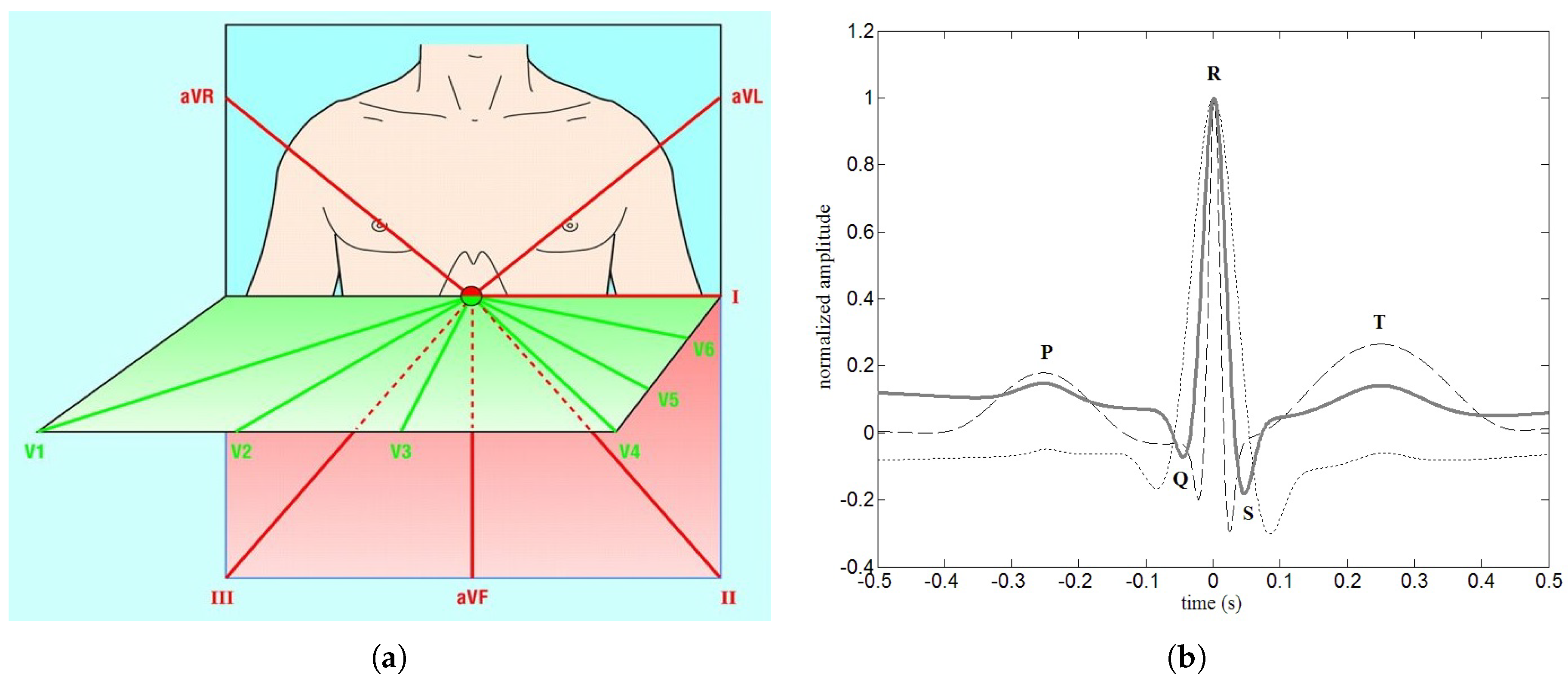
An $ECG$ originates following the atrial and ventricular contractions where the concentrations of the sodium and potassium ions are unbalanced so that the heart muscle, being electrically charged, is equivalent to an electric dipole vector with amplitude and variable direction during the depolarization and re-polarization of cells [8,17,27,28,29]. The electrical behavior of a single pair of ions produces an electrical dipole. All the electric dipoles determine a single resulting vector called Heart Dipole Vector (HDV), $\mathbf{d}\left(t\right)$, where t is the time variable. Then, an $ECG\left(t\right)$ derives from the scalar product between $\mathbf{d}\left(t\right)$ and the direction of the axis of the recording electrode, $\mathbf{v}$, generating the so-called Heart Dipole Model (HDM). On these premises, an $ECG$ consists of 12 different leads describing the same vector $\mathbf{d}\left(t\right)$ at the same instant t but from different points of view. $\mathbf{d}\left(t\right)$ reconstruction requires the analysis of its projection in several different leads, to identify its spatial arrangement within the heart. The electromotive forces are best recorded on the horizontal plane (left to right, parallel to the horizon) and on the vertical (frontal) plane, perpendicular to the shoulder line, from head to toe. Running an $ECG$ includes the following leads (Figure 1a) [30,31]: (1) six vertical leads (on the frontal plane): (a) bipolar leads of the limbs: I, II, III (Standard leads); (b) uni-polar leads of the augmented limbs: aVR, aVL, aVF (Goldberger leads); (2) six horizontal branches (on the horizontal plane). Uni-polar or chest wall precordial leads: $V_1$ to $V_6$ or $V_9$ (Wilson leads). Uni-polar leads are recorded by coupling a single $scanning$ electrode with a central terminal, while bipolar leads record the potential difference between two electrodes. Leads I, II, II are bipolar; leads aVR, AVL, aVF, and Wilson leads are uni-polar [30,31,32,33].

3. Structure of an $\mathit{ECG}$: Normal Conditions and Pathological Events

$ECG$ is the graphic reproduction of the electrical activity of the heart during its operation, recorded at the level of the body surface in which low intensity electric fields are present and can be recorded, which in the individual at rest are mainly due to periodic depolarization and re-polarization of the heart [30,31]. Thanks to the conversion of electrical energy into mechanical energy, electrical variations produce the movement of a writing system. The electrical energy is adequately amplified so as to be able to transcribe sufficiently large excursions to allow the recording of a readable signal. The deflections are imprinted on paper, which moves at a constant speed in contact with the system, which reports on the paper the waves recorded as a function of time. Simultaneously with the vertical oscillation of the lines produced by the variations in potential, the paper flows to the left. This synchronization makes it possible to bring the vertical movement back to a horizontal plane, recording the oscillations in relation to their duration over time. The principle on which the measurement of the electrical activity of the heart is based is physiological: the onset of impulses in the myocardium leads to the generation of potential differences that vary in space and time and which can be acquired through electrodes placed on the body surface. By convention, the $ECG$ trace is reported on graph paper with the time on the abscissa (one second every 25 mm) and the amplitude on the ordinate (one mV every 10 mm). $ECG$ consists of a series of waves [30,31]. The P wave corresponds to the depolarization of the atria and originates from the sinoatrial node. When the electrical impulse leaves the sinus node it produces the depolarization of the neighboring myofibrils which contract, and then continues to propagate in the radial sinus. The PR interval concerns the wave front which, passing through the atria, passes into the atrio-ventricular node (AV) within which the activated cells are few and the dipole generated is too weak to be registered [30,31,32,34,35]. As soon as the depolarization wave reaches the AV node, the electrical conduction slows down until the ventricular conduction system is reached. The QRS complex concerns a set of waves that follow one another, corresponding to the depolarization of the ventricles. The Q wave corresponds to the depolarization of the inter-ventricular septum, the vector produced goes from left to right. The R wave is a very high peak and corresponds to the depolarization of the apical part of the ventricles. The S wave is also small in size and corresponds to the depolarization of the basal and posterior regions of the left ventricle. The ST segment represents the period in which the ventricular cells are all depolarized and therefore no electrical movements are detectable until the beginning of re-polarization. As a result, the ST segment is usually isoelectric, i.e., placed on the base line of the trace from which it can move, upwards or downwards, by no more than 1 mm (equal to 0.1 mV). The T wave is the first wave of the re-polarization of the ventricles. It is not always identifiable because it can be of very small amplitude. The QT interval represents electrical systole, that is the time in which ventricular depolarization and re-polarization occurs. The U wave is a wave that is not always appreciable because it is often of minimal size. It is due to the re-polarization of the papillary muscles, which can be evidenced in the case of myocardial hypertrophy or altered dimensions of the ventricular cavities [30,31,32,34,35]. The most salient characters of the human $ECG$ are shown in

Table 1. Characteristics of an $ECG$.

Section	Duration (s)	Amplitude (mV)	Meaning
P Wave	0.07–0.12	0.2–0.4	Atrial Depolarization
QRS Complex	0.06–0.10	1–2	Depolarization of the intraventricular septum (Q)
			and ventricles (RS)
T Wave	0.18–0.20	0.4–0.5	Ventricular re-polarization
U Wave	0.08	-	Re-polarization of the Purkinje System
P-R Interval	0.1–0.20	-	Atrioventricular conduction time
S-T Interval	0.30	-	Duration of ventricular re-polarization
Q-T Interval	0.40	-	Duration of electrical ventricular systole
R-R Interval	0.8–0.9	-	Duration of cardiac cycle

([36]). Excitation initially spreads along the right atrium via the three inter-nodal tracts and reaches the AV node. The resulting atrial vector is directed from the upper right to the lower left, approximately in the same direction as the standard II lead. The PR interval runs from the beginning of the P wave to the beginning of the QRS complex (which represents the depolarization of the ventricles) [30,31,32,34] and indicates the time required for a pulse to travel from the sinus node to the ventricles and includes conduction through the atria and the AV node. This is the last element as certain drugs or pathologies can delay conduction through the atrioventricular node. A shortening of the P-R interval may indicate that conduction occurs through an accessory beam that “skips” the AV node. This phenomenon can be associated with atrial arrhythmia. The normal activation sequence occurs when the impulse runs from the AV node to the branches and to the Purkinje system [30,31,32,34]. The left branch is depolarized a little before the right branch because the initial depolarization vector runs from the left side to the right side of the septum. Initial septal activation produces the initial Q wave in left-directed leads I and VL, as well as in left thoracic leads $V_5$ and $V_6$. Subsequently, various areas of the left/right ventricle are activated simultaneously. When both ventricles are depolarized, there is no vector, and the R wave returns to the baseline. The point where the vector changes direction along the axis of the derivation of the electrocardiography leads is called deflection. The configuration of QRS in the bipolar and uni-polar leads of the limbs (frontal plane) depends on the axis of the heart. In precordial leads (horizontal plane) the amplitude of the R wave increases from $V_1$ to $V_5$ while at the same time, the amplitude of the S wave is reduced. The whole QRS complex may be a little smaller between $V_4$ and $V_6$, especially in patients with opiates or with pulmonary emphysema [30,31,32,33,34]. The T wave represents the depolarization of the ventricles, and it is larger than the QRS complex, with slightly asymmetrical branches and a rounded tip, mainly because re-polarization does not occur with the same course as depolarization. Generally, the T wave is positive in those leads where the QRS complex is predominantly positive. Figure 1b depicts $ECG$ signals, both normal and pathological ones [30,31,32,34].

4. HDV and 12-Leads $\mathit{ECG}$ System: A Brief Overview

Let us consider a region $\mathsf{\Omega }\subset {\mathbb{R}}^3$ endowed with a system of Cartesian axes $Oxyz$ in which the origin O represents the central area of the heart muscle (see Figure 1a). The unit orthogonal vectors are indicated by ${\widehat{\mathbf{i}}}_x$,${\widehat{\mathbf{i}}}_y$ and ${\widehat{\mathbf{i}}}_z$. Usually, the cardiac activity, referred to three orthogonal planes ($x-z$ plane (sagittal plane); $y-z$ plane (frontal plane) and $x-y$ plane (transverse plane)) can be simulated by an ad-hoc time-varying rotating vector [5] $\mathbf{d}\left(t\right)=(d_x\left(t\right),d_y\left(t\right),d_z\left(t\right))$ in which the Cartesian representation in the $Oxyz$ system is:

$$\mathbf{d}\left(t\right)=d_x\left(t\right){\widehat{\mathbf{i}}}_x+d_y\left(t\right){\widehat{\mathbf{i}}}_y+d_z\left(t\right){\widehat{\mathbf{i}}}_z.$$

(1)

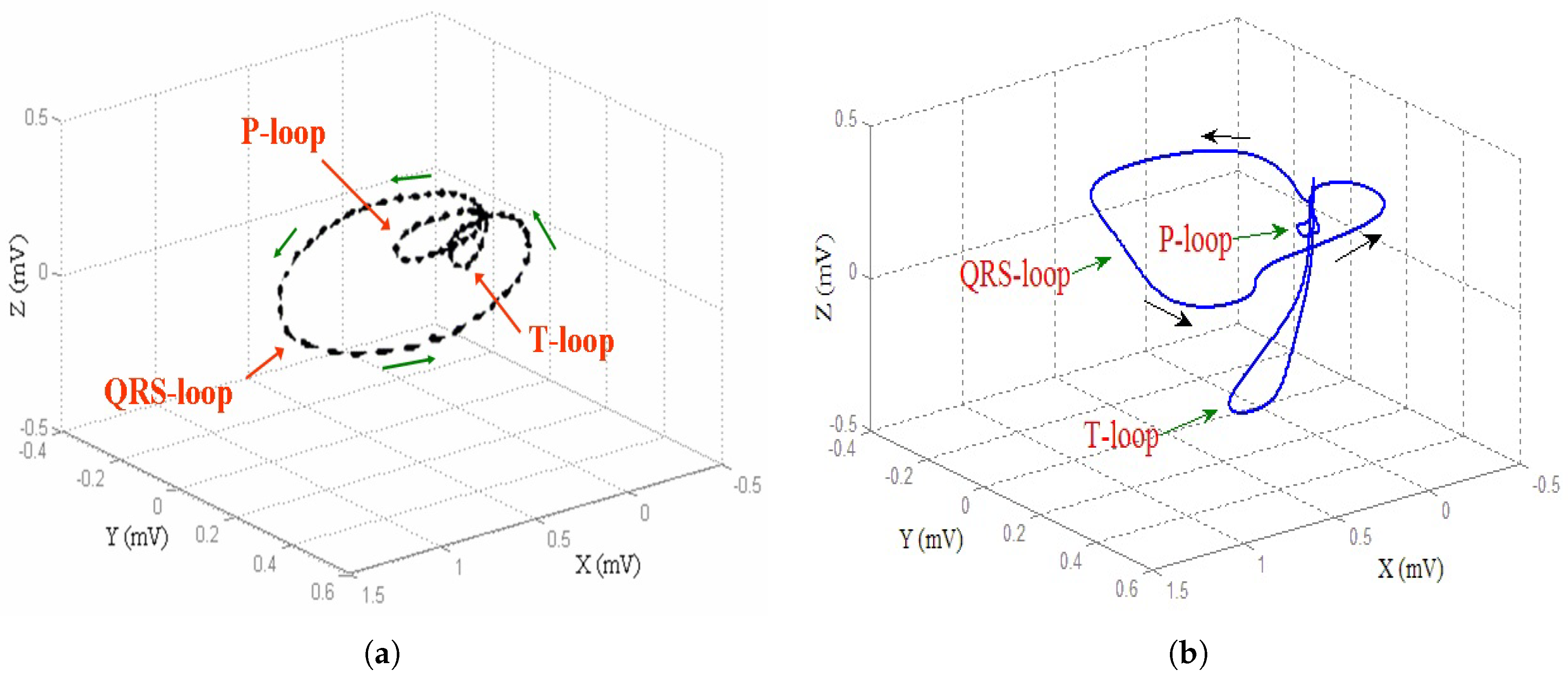
As $t\to +\infty$, $\mathbf{d}\left(t\right)$ varies cyclically in both amplitude and direction, keeping the origin fixed, depicting a 3D spatial loop in $Oxyz$ (the well-known VCG). As an example, Figure 2a displays a typical VCG loop during a normal cardiac cycle, while Figure 2b depicts the VCG loop with a nodal rhythm disease.

If $\mathbf{v}=v_x{\widehat{\mathbf{i}}}_x+v_y{\widehat{\mathbf{i}}}_y+v_z{\widehat{\mathbf{i}}}_z$ is the direction of the axis of the recording electrode, $ECG\left(t\right)$ can be written as follows:

$$ECG\left(t\right)=\mathbf{d}\left(t\right)·{\mathbf{v}}^T=v_x{d}_x\left(t\right)+v_y{d}_y\left(t\right)+v_z{d}_z\left(t\right).$$

(2)

In accordance with (1) and (2), it is possible to perform a description of the HDV 3D using three $ECG$ signals obtaining by the scalar product of $\mathbf{d}$ with each of coordinate axes ${\mathbf{v}}_1$, ${\mathbf{v}}_2$, ${\mathbf{v}}_3$.

Remark 1.

The single dipole model is not a perfect modeling of cardiac activity, so that the complete 12-lead $ECG$ system is useful (albeit redundant) for diagnosis.

The 12-lead $ECG$ system records the following 12 linearly independent signals: the three Einthoven points I, $II$, $III$; Wilson three leads $aVR$, $aVL$, $aVH$ and the six precordial leads $V1-V6$ [1,3]. However, to get a more detailed description of $ECG$ when noise, uncertainty and/or imprecision take place, we need to generalize Equation (2) considering a $3\times 3$ matrix $\mathbf{V}$, corresponding to the projection of the HDV onto the direction of the recording electrode, and a $12\times 3$ matrix, $\mathbf{H}$, that includes the body volume conductor model [1,13,17]. Then, the vector $\mathbf{ECG}{\left(t\right)}_{12-lead}$ can be achieved as follows:

$$\mathbf{ECG}{\left(t\right)}_{12-lead}=\mathbf{H}·\mathbf{V}·\mathbf{d}\left(t\right)+\mathbf{N}\left(t\right)$$

(3)

in which $\mathbf{N}\left(t\right)$, $\forall t$, represents a vector in which the components are the noise in each of the 12 $ECG$ channels. Equation (3) represents a mathematical model of the 12-lead $ECG$ system even when a pathology is in place. In the next section, we present a particular dynamic model in which the parameters are associated with certain cardiac pathologies.

Remark 2.

We observe that (3) is a typical procedure frequently used in dynamic systems (and in particular in signal processing theory) for the reconstruction of a signal in the time domain [25]. This procedure, as seen above, uses the formulation of matrices, $\mathbf{H}$, $\mathbf{V}$ and $\mathbf{N}$ as holding information contents typical of the system under study (including the components due to noise). Such matrices are usually very difficult to obtain. Therefore, this procedure is not practically exploitable to generate $ECG\left(t\right)$ in which cardiac pathologies could also be considered. Thus, for our purposes, we prefer starting from the well-known McSharry et al. dynamical model [24] to obtain a general $ECG\left(t\right)$ in which cardiac pathologies could also be taken into account.

5. The McSharry Dynamical Model

$ECG$ of Patients with Heart Disease: The McSharry Single Channel Modeling Approach

In [24], the $PQRST$ complex was obtained by a set of Gaussian functions with different parameters. If $s\left(t\right)$ is the $ECG$ signal, then:

$$\dot{s}\left(t\right)=-\sum _{i\in \{P,Q,R,S,T\}}{a}_i{|\theta -{\theta }_i|}_{2\pi }{e}^{-\frac{\left(\right|\theta -{\theta }_i{{|}_{2\pi })}^2}{2b_i^2}}-(s\left(t\right)-s_0\left(t\right))$$

(4)

where $\dot{s}\left(t\right)=\frac{ds\left(t\right)}{dt}$, ${\left|\right|}_{2\pi }$ is the module $2\pi$ operator and $({\alpha }_i,b_i,{\theta }_i)$ is a set of empirical parameters (see

Table 2. Experimental parameters for the McSharry dynamical model.

i	P	Q	R	S	T
time (s)	−0.250	−0.025	0	0.025	0.250
${\theta }_i$ (rad)	$-\pi /3$	$-\pi /12$	0	$\pi /12$	$\pi /2$
$a_i$	1.25	−5.00	30.00	−8.00	1.00
$b_i$	0.25	0.1	0.1	0.1	0.5

). Finally, $\theta$ represents an angular dynamic parameter that influences the deflections.

In [24], (4) was coupled with the following dynamical system:

$$\left\{\begin{array}{c}\dot{\chi }\left(t\right)=(1-\sqrt{{\chi }^2\left(t\right)+{\gamma }^2\left(t\right)})\chi \left(t\right)-\omega \gamma \left(t\right)\hfill \\ \dot{\gamma }\left(t\right)=(1-\sqrt{{\chi }^2\left(t\right)+{\gamma }^2\left(t\right)})\gamma \left(t\right)+\omega \chi \left(t\right)\hfill \end{array}\right.$$

(5)

in which $\omega$ is a parameter concerning the heart rate, obtaining the following dynamical model:

$$\left\{\begin{array}{c}\dot{\chi }\left(t\right)=(1-\sqrt{{\chi }^2\left(t\right)+{\gamma }^2\left(t\right)})\chi \left(t\right)-\omega \gamma \left(t\right)\hfill \\ \dot{\gamma }\left(t\right)=(1-\sqrt{{\chi }^2+{\gamma }^2\left(t\right)})\gamma \left(t\right)+\omega \chi \left(t\right)\hfill \\ \dot{s}\left(t\right)=-\sum _{i\in \{P,Q,R,S,T\}}{a}_i{|\theta -{\theta }_i|}_{2\pi }{e}^{-\frac{\left(\right|\theta -{\theta }_i{{|}_{2\pi })}^2}{2b_i^2}}-(s\left(t\right)-s_0\left(t\right))\hfill \end{array}\right.$$

(6)

where $s_0\left(t\right)=Asin\left(2\pi f_{0}t\right)$, with $A=0.15$ mV and $f_0$ ($s^{-1}$) respiratory frequency, is the artifact due to breathing. $\omega$ is the angular velocity of the trajectory [24]. Moreover, $\theta$ can be evaluated as follows [37]:

$$\theta =atan2(\gamma \left(t\right),\chi \left(t\right))=\left\{\begin{array}{c}\left(a\right)atan\left(\frac{\gamma \left(t\right)}{\chi \left(t\right)}\right),\chi \left(t\right)>0;\hfill \\ \left(b\right)atan\left(\frac{\gamma \left(t\right)}{\chi \left(t\right)}\right)+\pi ,\chi \left(t\right)<0\wedge \gamma \left(t\right)\ge 0\hfill \\ \left(c\right)atan\left(\frac{\gamma \left(t\right)}{\chi \left(t\right)}\right)-\pi ,\chi \left(t\right)<0\wedge \gamma \left(t\right)<0\hfill \\ \left(d\right)+\frac{\pi }{2},\chi \left(t\right)=0\wedge \gamma \left(t\right)>0\hfill \\ \left(e\right)-\frac{\pi }{2},\chi \left(t\right)=0\wedge \gamma \left(t\right)<0\hfill \\ \left(f\right)\mathrm{not}\mathrm{defined},\chi \left(t\right)=0\wedge \gamma \left(t\right)=0\hfill \end{array}\right.$$

(7)

so that $-\pi \le atan2\left(\gamma \right(t),\chi (t\left)\right)\le \pi$.

Remark 3.

$|atan2(\gamma \left(t\right),\chi \left(t\right))-{\theta }_i{|}_{2\pi }$ means that from the division between $atan2(\gamma ,\chi )-{\theta }_i$ and $2\pi$ only the rest must be considered. $atan2\left(\gamma \right(t),\chi (t\left)\right)$ indicates the angle between the positive semi-axis of X of a Cartesian plane and a point of coordinates $\left(\gamma \right(t),\chi (t\left)\right)$ lying on it. The angle is positive if counterclockwise (half plane of positive ordinates) and negative if clockwise (half plane of negative ordinates). The function is an extension of the $atan$ function since, unlike this, it distinguishes between diametrically opposite angles, not only considering the relationship between the arguments but also their sign.

Finally, the McSharry system (6) can be written in the following form:

$$\left\{\begin{array}{c}\dot{\chi }\left(t\right)=(1-\sqrt{{\chi }^2\left(t\right)+{\gamma }^2\left(t\right)})\chi \left(t\right)-\omega \gamma \left(t\right)\hfill \\ \dot{\gamma }\left(t\right)=(1-\sqrt{{\chi }^2\left(t\right)+{\gamma }^2\left(t\right)})\gamma \left(t\right)+\omega \chi \left(t\right)\hfill \\ \dot{s}\left(t\right)=-\sum _{i\in \{P,Q,R,S,T\}}{a}_i{|atan2(\gamma \left(t\right),\chi \left(t\right))-{\theta }_i|}_{2\pi }{e}^{-\frac{\left(\right|atan2(\gamma \left(t\right),\chi \left(t\right))-{\theta }_i{{|}_{2\pi })}^2}{2b_i^2}}-(s\left(t\right)-s_0\left(t\right))\hfill \end{array}\right.$$

(8)

Remark 4.

In [24], (5) was coupled with (4) without evaluating the presence of possibly equilibrium configurations for (5). In our work, unlike [24], we consider (5) as a system in which the solutions are the inputs for the Equation (4) where $s\left(t\right)$ represents the $ECG\left(t\right)$. Therefore, before studying the complete system (8), we study the stability of (5). This is because we have to verify that there are no traces of instability points (generating unbounded perturbations) on points admitted by (4). The following section proves how (5) admits an unstable equilibrium position, which does not belong to the set of points eligible for (4).

6. On the Stability of the System

6.1. On the Unique Equilibrium Position

The following result holds.

Proposition 1.

(5) admits the following unique equilibrium position:

$$({\chi }_0,{\gamma }_0)=(0,0).$$

(9)

Proof. 

The proof is based on the fact that if $({\chi }_0,{\gamma }_0)$ is an equilibrium position for (5), thus, $\forall t$, $(\chi \left(t\right),\gamma \left(t\right))=({\chi }_0,{\gamma }_0)$$(\dot{\chi }\left(t\right),\dot{\gamma }\left(t\right))=(0,0)$. For details, see Appendix A. □

6.2. On the Stability of the Unique Equilibrium Position

Proposition 2.

(9) is an unstable equilibrium position for (5).

Proof. 

(5) is nonlinear, so it was linearized (by Taylor series development). Afterward, the only position of equilibrium of the linearized system corresponding to the origin of the Cartesian axes was obtained. Applying the Lyapunov–Poincaré Lemma [38], it has been shown that the origin is also the only configuration of equilibrium for the nonlinearized system. Applying the first Lyapunov criterion, it has been shown that this equilibrium configuration is unstable. Therefore, these trajectories are not contained in closed curves on the phase plane. Hence the confirmation that the origin is an unstable equilibrium point. For details, see Appendix B. □

Remark 5.

We note that the only equilibrium configuration admitted by (5), (i.e., (9)) is located in the origin of the Cartesian axes. Furthermore, (9) does not belong to the domain of (7) because, in (9), (7) is not defined. Therefore, there is no instability points for (4).

In [24], (8) was solved using numerical techniques based on Runge–Kutta procedures. However, the solutions obtained could, in some cases, represent ghost solutions. In other words, the numerical procedure still provides a result that may not satisfy any analytical conditions of existence (and possibly uniqueness) of the solution. Thus, we need to verify that (8) still admits a solution and that it is unique. In this paper, we check if this happens.

7. The McSharry Dynamical Model: Existence and Uniqueness of the Solution

The uniqueness of the solution, from a clinical point of view, is very important as it ensures the one-to-one correspondence between a given pathology with a particular $ECG$.

We introduce the following definition.

Definition 1.

$f:{\mathbb{R}}^n\to {\mathbb{R}}^n$ defined on $X\subset {\mathbb{R}}^n$, with $X=\{x\ni x^{*}\le x\le x^{**}\}$, is said to be uniformly Lipschitzian if for it the ratio between the norm of the increases in f and that of the increases in x is maintained above limited. That is, there exists a number L (Lipschitz constant) such that $\{x\in X,x+\Delta x\in X\}$ from which $\{\parallel f(x+\Delta x)-f\left(x^{*}\right)\parallel \le L\parallel \Delta x\parallel \}$. The definition remains valid for a function $f(x,t)$ with $x\in X$ and with t set in T (real interval), and if then there exists a constant L for which it results that $x\in X,x+\Delta x\in X$, $t\in Tt+\Delta t\in T$, from which $\{\parallel f(x+\Delta x)-f\left(x^{*}\right)\parallel \le L\parallel \Delta x\parallel \}$, then, $f(x,t)$ is said to be uniformly Lipschitzian in $x\in X$ as t varies in T.

The following Lemma holds.

Lemma 1.

Let us consider the following Cauchy problem:

$$\left\{\begin{array}{c}\dot{x}\left(t\right)=f(x,t)\hfill \\ x\left(t_0\right)=x_0\hfill \end{array}\right.$$

(10)

in which $f(x,t)$ is continuous as $(x,t)$ varies in ${\mathbb{R}}^n\times T$, with T real interval, and uniformly Lipschitzian for $x\in {\mathbb{R}}^n$ with respect to $t\in T$. Then, however chosen $(t_0,x_0)\in X\times T$, (10) admits unique solution, $x\left(t\right)$.

Remark 6.

(8) can be written as (10). In fact, setting

$$\underline{\chi }\left(t\right)=\left(\begin{array}{c}\chi \left(t\right)\\ \gamma \left(t\right)\\ s\left(t\right)\end{array}\right);\dot{\underline{\chi }}=\left(\begin{array}{c}\dot{\chi }\left(t\right)\\ \dot{\gamma }\left(t\right)\\ \dot{s}\left(t\right)\end{array}\right);$$

(11)

$$\underline{h}(t,\underline{\chi }\left(t\right))=\left(\begin{array}{c}{h}_1(t,\underline{\chi }\left(t\right))\\ h_2(t,\underline{\chi }\left(t\right))\\ h_3(t,\underline{\chi }\left(t\right))\end{array}\right)=\left(\begin{array}{c}(1-\sqrt{{\chi }^2\left(t\right)+{\gamma }^2\left(t\right)})\chi \left(t\right)-\omega \gamma \left(t\right)\\ (1-\sqrt{{\chi }^2\left(t\right)+{\gamma }^2\left(t\right)})\gamma \left(t\right)+\omega \chi \left(t\right)\\ -\sum _{i\in \{P,Q,R,S,T\}}{a}_i|\theta -{\theta }_i{|}_{2\pi }{e}^{{(-\frac{|\theta -{\theta }_1{|}_{2\pi }}{\sqrt{2}{b}_i})}^2}+(s\left(t\right)-s_0\left(t\right))\end{array}\right),$$

(12)

we can write:

$$\left\{\begin{array}{c}\dot{\underline{\chi }}\left(t\right)=\underline{h}(t,\underline{\chi }\left(t\right))\hfill \\ \underline{\chi }\left(0\right)={\underline{\chi }}_0.\hfill \end{array}\right.$$

(13)

where $\underline{\chi }\left(0\right)={\underline{\chi }}_0$ are the initial conditions. The following results hold.

Proposition 3.

$\underline{h}(t,\underline{\chi }\left(t\right))$, as defined in (12), is continuous as $(t,\underline{\chi }\left(t\right))$ varies in ${\mathbb{R}}^3\times T$, with T real interval.

Proof. 

The proof is based on the verification of the continuity of each single addendum. For details, see Appendix C. □

Proposition 4.

$\underline{h}(t,\underline{\chi }\left(t\right))$, is uniformly Lipschitzian.

Proof. 

For details, see Appendix D. □

Theorem 1.

System (8) admits unique solution.

Proof. 

It immediately follows from Propositions 3 and 4 and from Lemma 1. □

Remark 7.

The resolution of (8) is usually numeric and techniques based on Runge–Kutta procedures are particularly suitable for this goal [24]. However, different values of $atan2\left(\gamma \right(t),\chi (t\left)\right)$ (see (7)) provide different formulations with consequent different solution. Then, in the following Section the McSharry models obtained for different values of $atan2\left(\gamma \right(t),\chi (t\left)\right)$ are presented and solved.

8. The McSharry Dynamical Model and the Study of the Trajectory: Peculiarities and Weaknesses

8.1. Case (a): $\chi \left(t\right)>0$, $atan2(\gamma \left(t\right),\chi \left(t\right))=atan\left(\frac{\gamma \left(t\right)}{\chi \left(t\right)}\right)$

Here, taking into account (7), it follows that $atan2(\gamma \left(t\right),\chi \left(t\right))=atan\left(\frac{\gamma \left(t\right)}{\chi \left(t\right)}\right)$, and considering the values in Table 2, (8) becomes:

$$\left\{\begin{array}{c}\dot{\chi }\left(t\right)=(1-\sqrt{{\chi }^2\left(t\right)+{\gamma }^2\left(t\right)})\chi \left(t\right)-\omega \gamma \left(t\right)\hfill \\ \dot{\gamma }\left(t\right)=(1-\sqrt{{\chi }^2\left(t\right)+{\gamma }^2\left(t\right)})\gamma \left(t\right)+\omega \chi \left(t\right)\hfill \\ \dot{s}\left(t\right)=-5(s\left(t\right)-0.15\left(2\pi f_{2}t\right))-1.1|atan\left(\frac{\gamma \left(t\right)}{\chi \left(t\right)}\right)+\frac{\pi }{3}{|}_{2\pi }{e}^{-{\left(\frac{|atan\left(\frac{\gamma \left(t\right)}{\chi \left(t\right)}\right)+\frac{\pi }{3}{|}_{2\pi }}{0.25\sqrt{2}}\right)}^2}-\hfill \\ -5|atan\left(\frac{\gamma \left(t\right)}{\chi \left(t\right)}\right)+\frac{\pi }{12}{|}_{2\pi }{e}^{-{\left(\frac{|atan\left(\frac{\gamma \left(t\right)}{\chi \left(t\right)}\right)+\frac{\pi }{12}{|}_{2\pi }}{0.1\sqrt{2}}\right)}^2}-30|atan\left(\frac{\gamma \left(t\right)}{\chi \left(t\right)}\right){|}_{2\pi }{e}^{-{\left(\frac{|atan\left(\frac{\gamma \left(t\right)}{\chi \left(t\right)}\right){|}_{2\pi }}{0.1\sqrt{2}}\right)}^2}+\hfill \\ +7.5|atan\left(\frac{\gamma \left(t\right)}{\chi \left(t\right)}\right)-\frac{\pi }{12}{|}_{2\pi }{e}^{-{\left(\frac{|atan\left(\frac{\gamma \left(t\right)}{\chi \left(t\right)}\right)-\frac{\pi }{12}{|}_{2\pi }}{0.1\sqrt{2}}\right)}^2}+0.75|atan\left(\frac{\gamma \left(t\right)}{\chi \left(t\right)}\right)-\frac{\pi }{2}{|}_{2\pi }{e}^{-{\left(\frac{|atan\left(\frac{\gamma \left(t\right)}{\chi \left(t\right)}\right)-\frac{\pi }{-}{|}_{2\pi }}{0.4\sqrt{2}}\right)}^2}.\hfill \end{array}\right.$$

(14)

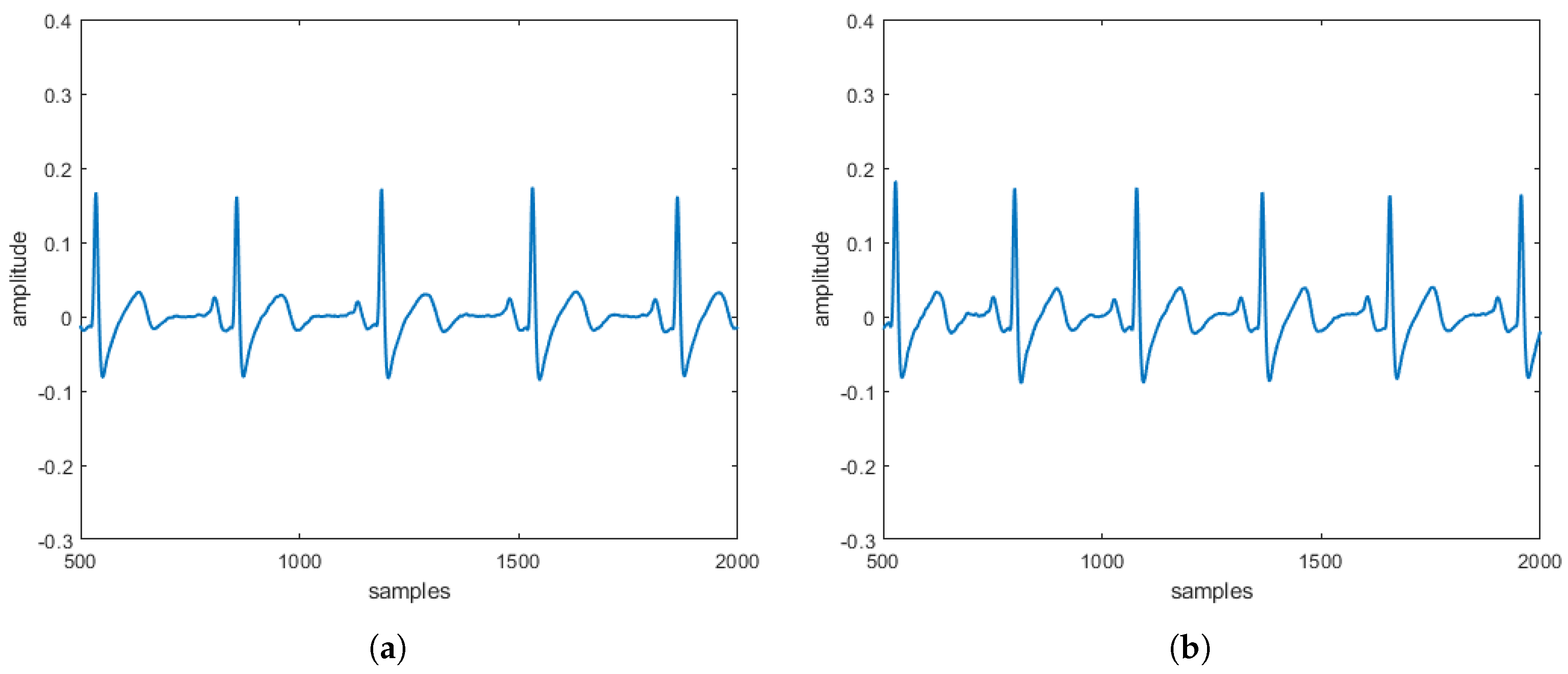
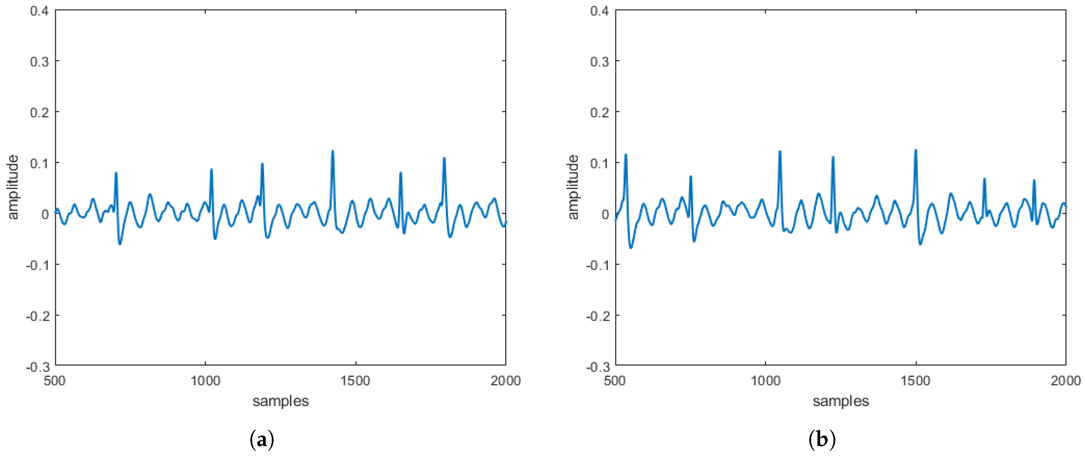
The numerical solution of (14), achieved by four-stage Lobatto IIa formula because it is a particularly suitable technique for solving nonlinear differential problems (for detail, see Appendix G), is depicted in Figure 3a, which shows the regular trend of the $ECG\left(t\right)$: the waves and relative deflections are clearly visible and determined by the periodic terms contained in $\dot{s}\left(t\right)$.

8.2. Case (b): $\chi \left(t\right)<0$ ∧ $\gamma \left(t\right)>0$, $atan2(\gamma \left(t\right),\chi \left(t\right))=atan\left(\frac{\gamma \left(t\right)}{\chi \left(t\right)}\right)+\pi$

In this case, considering (7), (8) becomes:

$$\left\{\begin{array}{c}\dot{\chi }\left(t\right)=(1-\sqrt{{\chi }^2\left(t\right)+{\gamma }^2\left(t\right)})\chi \left(t\right)-\omega \gamma \hfill \\ \dot{\gamma }\left(t\right)=(1-\sqrt{{\chi }^2\left(t\right)+{\gamma }^2\left(t\right)})\gamma +\omega \chi \hfill \\ \dot{s}\left(t\right)=-5(s\left(t\right)-0.15\left(2\pi f_{2}t\right))-1.1|atan\left(\frac{\gamma \left(t\right)}{\chi \left(t\right)}\right)+\frac{4\pi }{3}{|}_{2\pi }{e}^{-{\left(\frac{|atan\left(\frac{\gamma \left(t\right)}{\chi \left(t\right)}\right)+\frac{4\pi }{3}{|}_{2\pi }}{0.25\sqrt{2}}\right)}^2}-\hfill \\ -5|atan\left(\frac{\gamma \left(t\right)}{\chi \left(t\right)}\right)+\frac{13\pi }{12}{|}_{2\pi }{e}^{-{\left(\frac{|atan\left(\frac{\gamma \left(t\right)}{\chi \left(t\right)}\right)+\frac{13\pi }{12}{|}_{2\pi }}{0.1\sqrt{2}}\right)}^2}-30|atan\left(\frac{\gamma \left(t\right)}{\chi \left(t\right)}\right){|}_{2\pi }{e}^{-{\left(\frac{|atan\left(\frac{\gamma \left(t\right)}{\chi \left(t\right)}\right){|}_{2\pi }}{0.1\sqrt{2}}\right)}^2}+\hfill \\ +7.5|atan\left(\frac{\gamma \left(t\right)}{\chi \left(t\right)}\right)-\frac{11\pi }{12}{|}_{2\pi }{e}^{-{\left(\frac{|atan\left(\frac{\gamma \left(t\right)}{\chi \left(t\right)}\right)-\frac{\pi }{12}{|}_{2\pi }}{0.1\sqrt{2}}\right)}^2}+0.75|atan\left(\frac{\gamma \left(t\right)}{\chi \left(t\right)}\right)-\frac{\pi }{2}{|}_{2\pi }{e}^{-{\left(\frac{|atan\left(\frac{\gamma \left(t\right)}{\chi \left(t\right)}\right)-\frac{\pi }{-}{|}_{2\pi }}{0.4\sqrt{2}}\right)}^2}.\hfill \end{array}\right.$$

(15)

Also in this case the periodic terms contained in $\dot{s}\left(t\right)$ produce the deflections in the corresponding $ECG$. However, the presence of noise components (mainly due to the particular value of operative parameters in $\dot{s}\left(t\right)$) would require the use of suitable filters (see Figure 3b).

8.3. Case (c): $\chi \left(t\right)<0$ ∧ $\gamma \left(t\right)<0$, $atan2(\gamma \left(t\right),\chi \left(t\right))=atan\left(\frac{\gamma \left(t\right)}{\chi \left(t\right)}\right)-\pi$

In this case, considering (7), (8) assumes the following form:

$$\left\{\begin{array}{c}\dot{\chi }\left(t\right)=(1-\sqrt{{\chi }^2\left(t\right)+{\gamma }^2\left(t\right)})\chi \left(t\right)-\omega \gamma \hfill \\ \dot{\gamma }\left(t\right)=(1-\sqrt{{\chi }^2\left(t\right)+{\gamma }^2\left(t\right)})\gamma +\omega \chi \hfill \\ \dot{s}\left(t\right)=-5(s\left(t\right)-0.15\left(2\pi f_{2}t\right))-1.1|atan\left(\frac{\gamma \left(t\right)}{\chi \left(t\right)}\right)+\frac{4\pi }{3}{|}_{2\pi }{e}^{-{\left(\frac{|atan\left(\frac{\gamma \left(t\right)}{\chi \left(t\right)}\right)+\frac{4\pi }{3}{|}_{2\pi }}{0.25\sqrt{2}}\right)}^2}-\hfill \\ -5|atan\left(\frac{\gamma \left(t\right)}{\chi \left(t\right)}\right)+\frac{13\pi }{12}{|}_{2\pi }{e}^{-{\left(\frac{|atan\left(\frac{\gamma \left(t\right)}{\chi \left(t\right)}\right)+\frac{13\pi }{12}{|}_{2\pi }}{0.1\sqrt{2}}\right)}^2}-30|atan\left(\frac{\gamma \left(t\right)}{\chi \left(t\right)}\right){|}_{2\pi }{e}^{-{\left(\frac{|atan\left(\frac{\gamma \left(t\right)}{\chi \left(t\right)}\right){|}_{2\pi }}{0.1\sqrt{2}}\right)}^2}+\hfill \\ +7.5|atan\left(\frac{\gamma \left(t\right)}{\chi \left(t\right)}\right)-\frac{11\pi }{12}{|}_{2\pi }{e}^{-{\left(\frac{|atan\left(\frac{\gamma \left(t\right)}{\chi \left(t\right)}\right)-\frac{\pi }{12}{|}_{2\pi }}{0.1\sqrt{2}}\right)}^2}+0.75|atan\left(\frac{\gamma \left(t\right)}{\chi \left(t\right)}\right)-\frac{\pi }{2}{|}_{2\pi }{e}^{-{\left(\frac{|atan\left(\frac{\gamma \left(t\right)}{\chi \left(t\right)}\right)-\frac{\pi }{-}{|}_{2\pi }}{0.4\sqrt{2}}\right)}^2}.\hfill \end{array}\right.$$

(16)

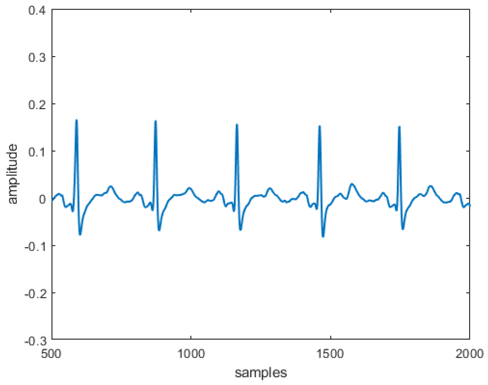
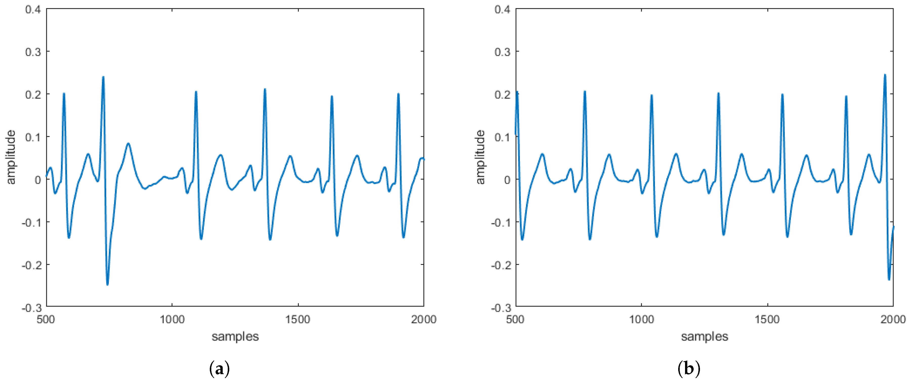
Like the two previous ones, it produces a regular $ECG$ signal in which waves and deflections are clearly visible (see Figure 4a). However, due to the operating parameters used, the signal amplitude appears reduced (albeit slightly).

8.4. Case (d): $\chi \left(t\right)=0$ ∧ $\gamma \left(t\right)>0$, $atan2(\gamma \left(t\right),\chi \left(t\right))=\frac{\pi }{2}$

In this case, system (8) becomes:

$$\left\{\begin{array}{c}\dot{\gamma }\left(t\right)=(1-\gamma \left(t\right))\gamma \left(t\right)\hfill \\ \dot{s}\left(t\right)=-8.10e^{-21}-5(z\left(t\right)-0.15\left(2\pi f_{2}t\right)).\hfill \end{array}\right.$$

(17)

However, (17) is simple to solve analytically by obtaining the following solution (for analytical details, see Appendix E):

$$\left\{\begin{array}{c}\gamma \left(t\right)=\frac{K_2{e}^t}{K_2{e}^t-1}\hfill \\ s\left(t\right)=e^{-5t}\left\{C+0.75\frac{-\frac{1}{5}sin\left(2\pi f_{2}t\right)-\frac{2\pi f_2}{25}{e}^{-5t}cos\left(2\pi f_{2}t\right)}{1+{\left(\frac{2\pi f_2}{5}\right)}^2}-8.10e^{-21}t\right\}\hfill \end{array}\right.$$

(18)

where $K_2$ and C are constant. We immediately notice that, as $t\to +\infty$, form system (18), $\gamma \left(t\right)\to 1$ and $s\left(t\right)\to 0$ so that the expected periodicity vanishes. Thus, this case must be discarded.

8.5. Case (e): $\chi \left(t\right)=0$, $\gamma \left(t\right)<0$, $atan2(\gamma \left(t\right),\chi \left(t\right))=-\frac{\pi }{2}$

In this case, system (8) becomes:

$$\left\{\begin{array}{c}\dot{\gamma }\left(t\right)=(1-\gamma \left(t\right))\gamma \left(t\right)\hfill \\ \dot{s}\left(t\right)=1.1e^{-{\left(-\frac{1}{0.25\sqrt{2}}\right)}^2}-(s\left(t\right)-0.15sin\left(2\pi f_{2}t\right)).\hfill \end{array}\right.$$

(19)

Here the solution is similar to the previous case therefore the respective system, as the previous case, results decoupled. Furthermore, the periodicity of the solution, excluding the respiratory artifact, has completely disappeared. Thus, also this case must be discarded.

8.6. Case (f): $\chi \left(t\right)=\gamma \left(t\right)=0$, $atan2\left(\gamma \right(t),\chi (t\left)\right)$ Not Defined

We note that if $\chi \left(t\right)=\gamma \left(t\right)=0$, it follows that $atan2\left(\gamma \right(t),\chi (t\left)\right)$ is not defined (see option $\left(f\right)$ in (7)). Moreover, $\chi \left(t\right)=\gamma \left(t\right)=0$ corresponds to the equilibrium position for (5) that results to be unstable. So that, in (7), position $\chi \left(t\right)=0\wedge \gamma \left(t\right)=0$ must be discarded.

Remark 8.

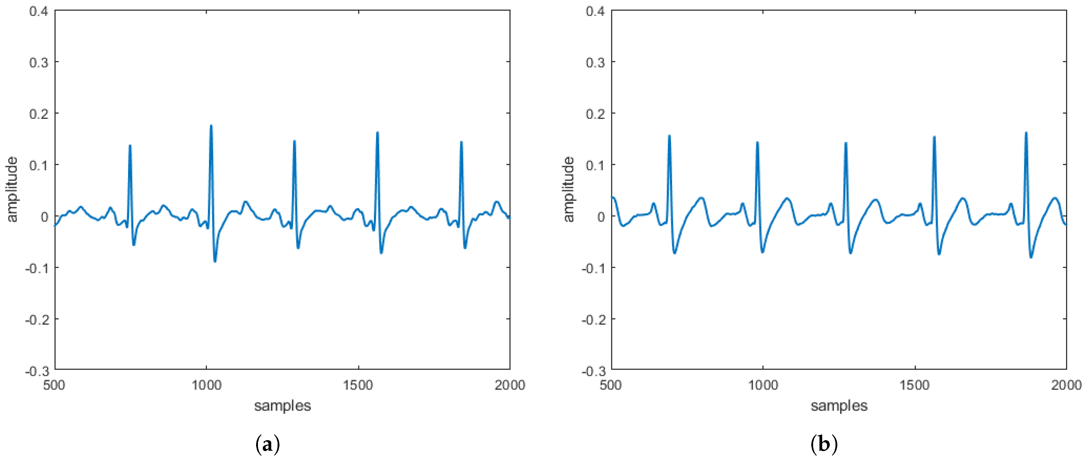
It is worth observing how the $ECG$s obtained by numerical solution of McSharry models (see Figure 3a,b and Figure 4a) are qualitatively quite similar to the $ECG$s obtained by clinical investigation of patients not affected by pathologies (a typical $ECG$ related to a subject not affected by pathologies is shown in Figure 4b). However, a quantification of this similarity is required. In this regard, please refer to Section 10.

Remark 9.

As $atan2\left(\gamma \right(t),\chi (t\left)\right)$ varies according to (7), we have six different McSharry systems. However, only three of them provided reliable results from a biomedical point of view. In particular, only (a), (b) and (c) cases in Section 8 provide reliable $ECG\left(t\right)$. Excluding the case (f) where $atan2\left(\gamma \right(t),\chi (t\left)\right)$ is not defined, cases (d) and (e) provide physically unreliable results because there $atan2(\gamma \left(t\right),\chi \left(t\right))=\pm \frac{\pi }{2}$. Finally, due to its structure, the McSharry model is unable to simulate $ECG\left(t\right)$ affected by heart disease. Therefore it is necessary to modify this model to take into account the possible alterations due to cardiac pathologies. Section 9 presents a new approach to modifying McSharry model in order to take into account heart diseases.

9. The Modified Heart Dipole Model (MHDM)

McSharry and co-authors were not able to characterize the distortion of the $PQRST$ complex [24]. Then, we propose a generalization of the $\chi -\gamma$ limit orbit by modifying (5) so that this limit orbit can be dynamically adapted. To simulate pathological $ECG$ signals, it is essential to choose a set of parameters that act as a controller of the limit orbit generalization. So, we here propose to generalize the limit cycle by an elliptic orbit introducing a linear transformation and a rotation:

$$\left(\begin{array}{c}\widehat{\chi }\left(t\right)\\ \widehat{\gamma }\left(t\right)\end{array}\right)=\underset{rotation}{\underbrace{\left(\begin{array}{cc}cos\varphi & sin\varphi \\ -sin\varphi & cos\varphi \end{array}\right)}}·\underset{lineartransformation}{\underbrace{\left(\begin{array}{cc}{k}_1& 0\\ 0& k2\end{array}\right)·\left(\begin{array}{c}\chi \left(t\right)\\ \gamma \left(t\right)\end{array}\right)}}$$

(20)

so that $\theta =atan2(\widehat{\gamma }\left(t\right),\widehat{\chi }\left(t\right))$, with $\widehat{\gamma }\left(t\right)$ and $\widehat{\chi }\left(t\right)$ computed by (20). Moreover, we note that for $k_1=k_2=1$ and $\varphi =0$, (20) does not modify (5). We also note that, as the parameters $k_1$, $k_2$ and $\varphi$ vary, the PQRST complex undergoes a distortion. Therefore, for certain values of $k_1$, $k_2$ and $\varphi$ it is possible to simulate specific heart diseases.

Table 3. Some synthetic diseases by the modified heart dipole model (MHDM).

Model Parameters	PQRST Complex Alteration	Correlated Disease
$k_1=1$, $k_2=1$, $\varphi =0$	-	normal sinus rhythm
$k_1=0.3$, $k_2=0.1$, $\varphi =\pi /8$	rapid ventricular	atrial fibrillation
	rate normal QRS
$k_1=0.5$, $k_2=0.1$, $\varphi =\pi /4$	isoelectric interval TP	atrial flutter
$k_1=0.2$, $k_2=0.3$, $\varphi =\frac{2}{3}\pi$	abnormal QRS	premature
	P wave not associated	ventricle contraction

shows some heart diseases associated with specific values of $k_1$, $k_2$ and $\varphi$.

Remark 10.

Also system (20) admits as its unique equilibrium position the origin O (see Proposition 5) verifying that the choice to use a linear transformation and a rotation does not affect the stability of the starting model. In other words, linear transformation and rotation do not generate instabilities different from the one already detected for (5) and therefore can be eliminated since the associated point is outside the domain of (7). Moreover, (20) has a twofold advantage: the computational complexity of the model is almost unvaried and, in addition, it is possible to characterize the distortion of the $PQRST$ complex setting $k_1$, $k_2$ and ϕ.

Then, the following result holds.

Proposition 5.

System (20) admits, as unique equilibrium point, the point (9).

Proof. 

For details, see Appendix F. □

MHDM Modelization

Staring from model (8) and considering the transformation (20) we can easily write:

$$\left\{\begin{array}{c}\dot{\widehat{\chi }}\left(t\right)=(1-\sqrt{{(k_1\chi \left(t\right)cos\varphi +k_2\gamma \left(t\right)sin\varphi )}^2+{(-k_1\chi \left(t\right)sin\varphi +k_2\gamma \left(t\right)cos\varphi )}^2})·\hfill \\ ·(k_1\chi \left(t\right)cos\varphi +k_2\gamma \left(t\right)sin\varphi )-\omega (-k_1\chi \left(t\right)sin\varphi +k_2\gamma \left(t\right)cos\varphi )\hfill \\ \dot{\widehat{\gamma }}\left(t\right)=(1-\sqrt{{(k_1\chi \left(t\right)cos\varphi +k_2\gamma \left(t\right)sin\varphi )}^2+{(-k_1\chi \left(t\right)sin\varphi +k_2\gamma \left(t\right)cos\varphi )}^2})·\hfill \\ ·(-k_1\chi \left(t\right)sin\varphi +k_2\gamma \left(t\right)cos\varphi )+\omega (k_1\chi \left(t\right)cos\varphi +k_2\gamma \left(t\right)sin\varphi )\hfill \\ \dot{s}\left(t\right)=-\sum _{i\in \{P,Q,R,S,T\}}{a}_i{|atan2(-k_1\chi \left(t\right)sin\varphi +k_2\gamma \left(t\right)cos\varphi ,k_1\chi \left(t\right)cos\varphi +k_2\gamma \left(t\right)sin\varphi )-{\theta }_i|}_{2\pi }·\hfill \\ ·e^{-\frac{\left(\right|atan2(-k_1\chi \left(t\right)sin\varphi +k_2\gamma \left(t\right)cos\varphi ,k_1\chi \left(t\right)cos\varphi +k_2\gamma \left(t\right)sin\varphi )-{\theta }_i{{|}_{2\pi })}^2}{2b_i^2}}-(s\left(t\right)-s_0\left(t\right)).\hfill \end{array}\right.$$

(21)

in which the parameters present have the same meaning as the cases studied above. System (21) admits different formulations as $|atan2(-k_1\chi \left(t\right)sin\varphi +k_2\gamma \left(t\right)cos\varphi ,k_1\chi \left(t\right)cos\varphi +k_2\gamma \left(t\right)sin\varphi )-{\theta }_i|$ varies according the (7). Thus, as obtained before in Section 8, we here achieve six formulations of system (21) depending on (7):

• Case (a):
  $k_1\chi \left(t\right)cos\varphi +k_2\gamma \left(t\right)sin\varphi >0$,
  $atan2(-k_1\chi \left(t\right)sin\varphi +k_2\gamma \left(t\right)cos\varphi ,k_1\chi \left(t\right)cos\varphi +k_2\gamma \left(t\right)sin\varphi )=$
  $=atan\left(\frac{-k_1\chi \left(t\right)sin\varphi +k_2\gamma \left(t\right)cos\varphi }{k_1\chi \left(t\right)cos\varphi +k_2\gamma \left(t\right)sin\varphi }\right)$;
• Case (b):
  $k_1\chi \left(t\right)cos\varphi +k_2\gamma \left(t\right)sin\varphi <0\wedge -k_1\chi \left(t\right)sin\varphi +k_2\gamma \left(t\right)cos\varphi >0$,
  $atan2(-k_1\chi \left(t\right)sin\varphi +k_2\gamma \left(t\right)cos\varphi ,k_1\chi \left(t\right)cos\varphi +k_2\gamma \left(t\right)sin\varphi )=$
  $=atan\left(\frac{-k_1\chi \left(t\right)sin\varphi +k_2\gamma \left(t\right)cos\varphi }{k_1\chi \left(t\right)cos\varphi +k_2\gamma \left(t\right)sin\varphi }\right)+\pi$;
• Case (c):
  $k_1\chi \left(t\right)cos\varphi +k_2\gamma \left(t\right)sin\varphi <0\wedge -k_1\chi \left(t\right)sin\varphi +k_2\gamma \left(t\right)cos\varphi <0$,
  $atan2(-k_1\chi \left(t\right)sin\varphi +k_2\gamma \left(t\right)cos\varphi ,k_1\chi \left(t\right)cos\varphi +k_2\gamma \left(t\right)sin\varphi )=$
  $=atan\left(\frac{-k_1\chi \left(t\right)sin\varphi +k_2\gamma \left(t\right)cos\varphi }{k_1\chi \left(t\right)cos\varphi +k_2\gamma \left(t\right)sin\varphi }\right)-\pi$;
• Case (d):
  $k_1\chi \left(t\right)cos\varphi +k_2\gamma \left(t\right)sin\varphi =0\wedge -k_1\chi \left(t\right)sin\varphi +k_2\gamma \left(t\right)cos\varphi >0$,
  $atan2(-k_1\chi \left(t\right)sin\varphi +k_2\gamma \left(t\right)cos\varphi ,k_1\chi \left(t\right)cos\varphi +k_2\gamma \left(t\right)sin\varphi )=\frac{\pi }{2}$;
• Case (e):
  $k_1\chi \left(t\right)cos\varphi +k_2\gamma \left(t\right)sin\varphi =0\wedge -k_1\chi \left(t\right)sin\varphi +k_2\gamma \left(t\right)cos\varphi <0$,
  $atan2(-k_1\chi \left(t\right)sin\varphi +k_2\gamma \left(t\right)cos\varphi ,k_1\chi \left(t\right)cos\varphi +k_2\gamma \left(t\right)sin\varphi )=-\frac{\pi }{2}$;
• Case (f):
  $k_1\chi \left(t\right)cos\varphi +k_2\gamma \left(t\right)sin\varphi =-k_1\chi \left(t\right)sin\varphi +k_2\gamma \left(t\right)cos\varphi =0$,
  $atan2(-k_1\chi \left(t\right)sin\varphi +k_2\gamma \left(t\right)cos\varphi ,k_1\chi \left(t\right)cos\varphi +k_2\gamma \left(t\right)sin\varphi )$ not defined

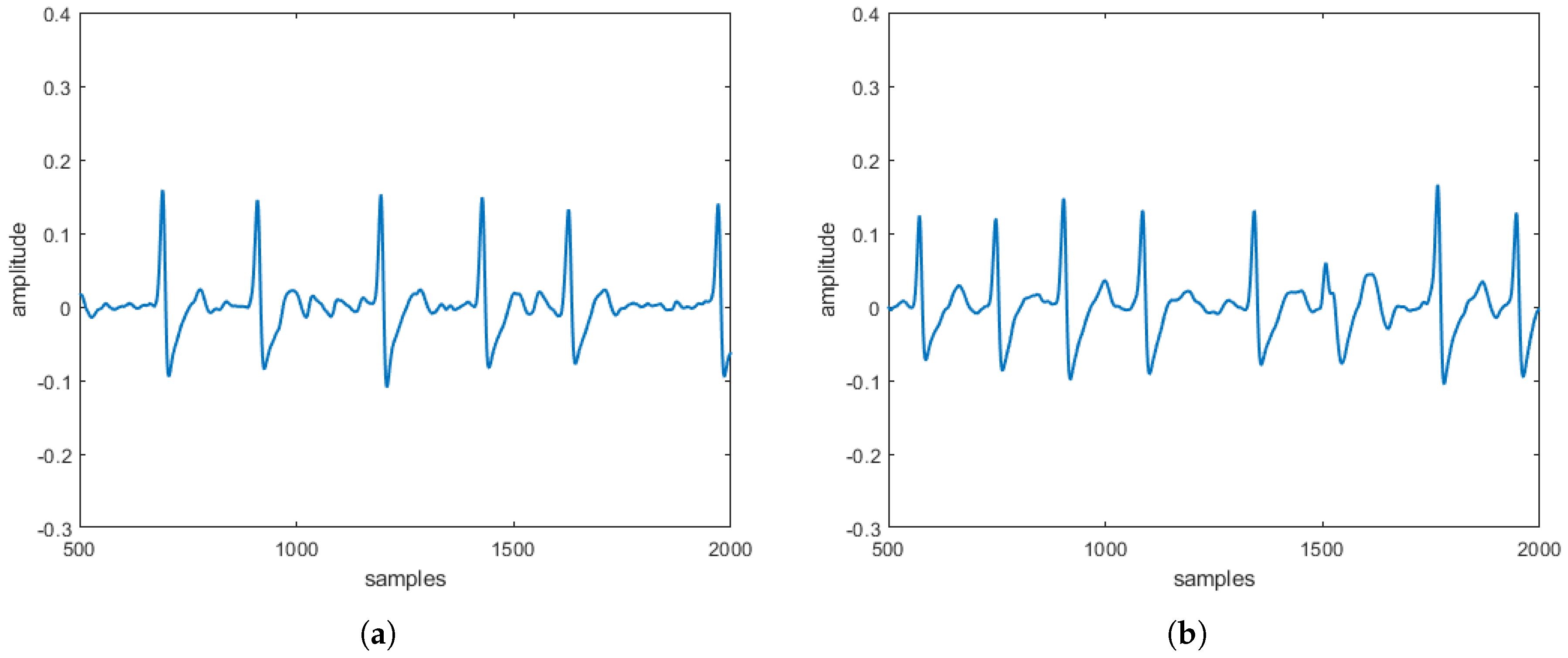
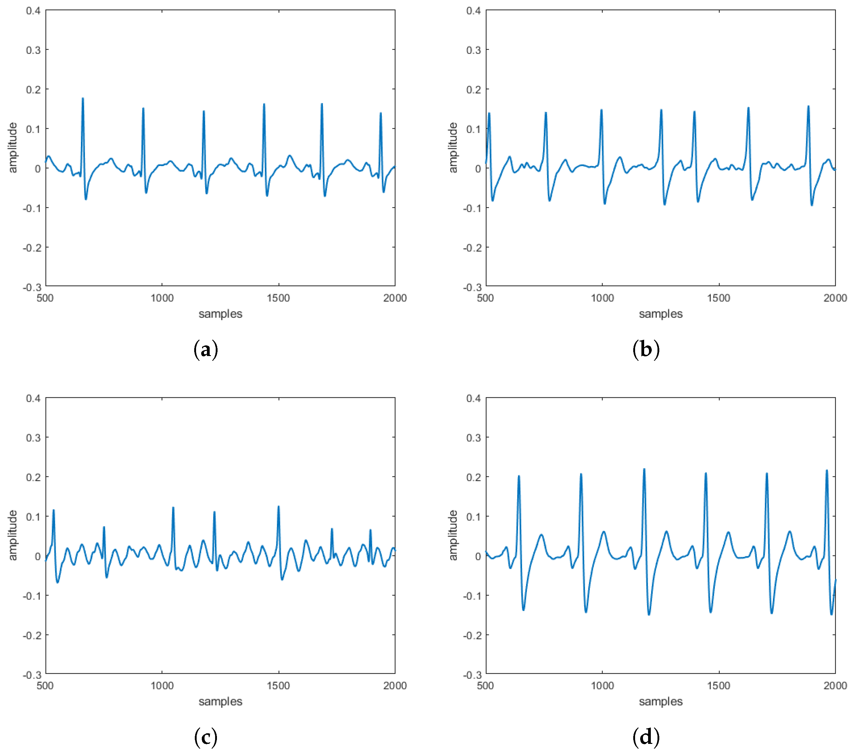
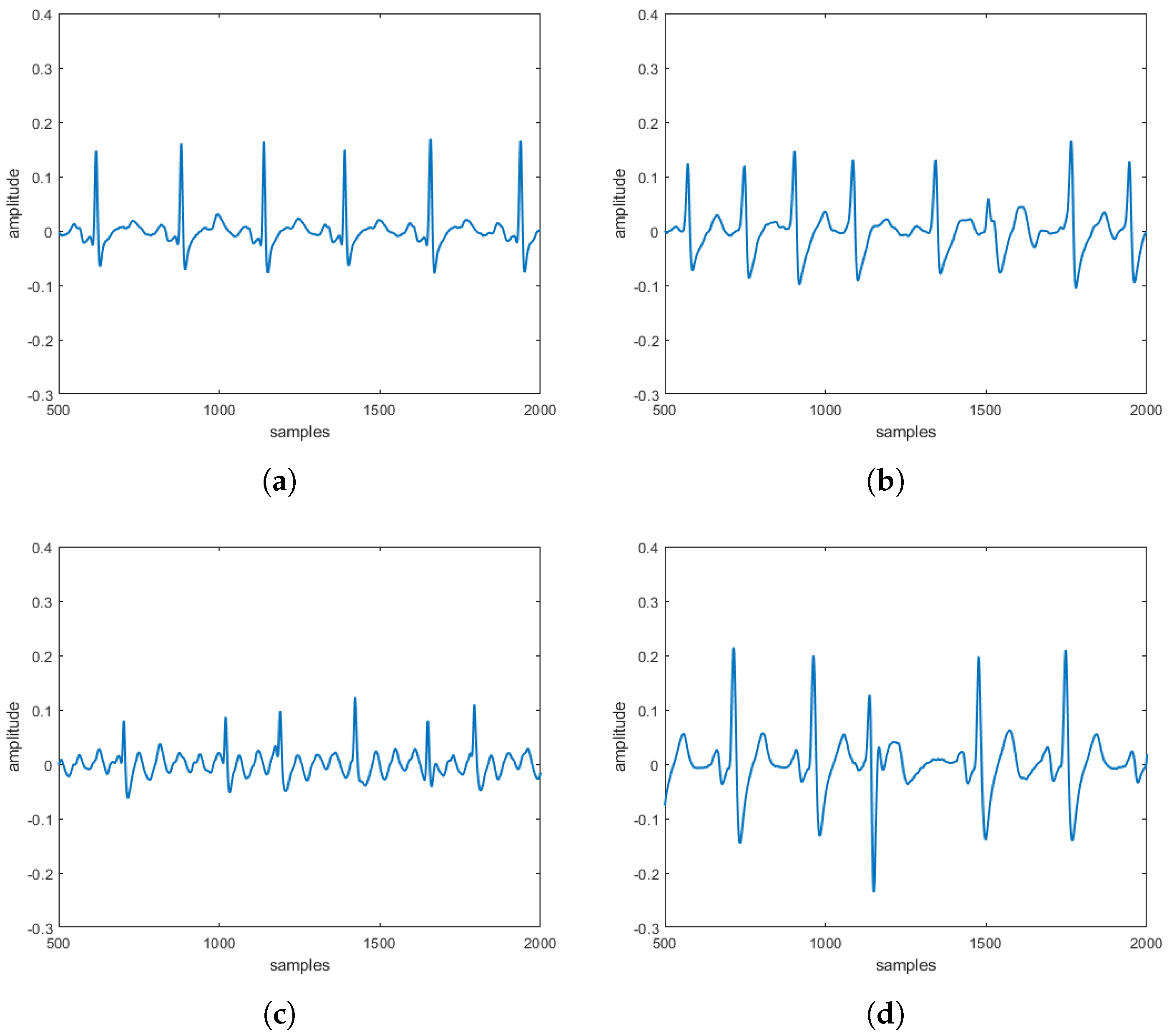
from which, by calculations completely similar to those made in Section 8, cases (d), (e) and (f) can be discarded. For each case we obtain a new formulation of the system (21) completely analogous to the formulations (14)–(16), respectively. For cases (a), (b) and (c) values of parameters $k_1$ and $k_2$ were considered such as to simulate normal conditions of heart rhythm and pathologies (atrial fibrillation, atrial flutter and premature contraction of the ventricle because they represent frequent pathologies in patients who are often highly at risk, having no obvious symptoms) as described in Table 3. By means of the four-stage Lobatto IIIa formula each system was numerically solved (for details, see Appendix G). Concerning the Case (a), Figure 5, Figure 6a, Figure 7a and Figure 8a display the $ECG$ obtained by varying $k_1$ and $k_2$ as per Table 3. $ECG\left(t\right)$ strongly adhering to real cases are highlighted, for which the methodology proposed to simulate $ECG$ pathologists provides qualitatively reliable results. Similarly, concerning Case (b) and (c) of the proposed methodology we also obtain $ECG$ conforming to real cases (see Figure 9a–d and Figure 10a–d).

Remark 11.

For Case (a) it is useful to observe that the numerically obtained $ECG$s are completely qualitatively similar to the $ECG$s sampled directly on patients as evidenced by the comparison between the Figure 4b and Figure 5; between Figure 6a,b; between Figure 7a,b and, finally, between Figure 8a,b. The same comparisons can be made for Case (b): it is sufficient to compare Figure 9a–d, with Figure 4b, Figure 6b, Figure 7b and Figure 8b respectively. Analogously, concerning Case (c), it is sufficient to compare Figure 10a–d with Figure 4b, Figure 6b, Figure 7b and Figure 8b respectively. Also in these cases, for the quantitative comparison, see Section 10.

Remark 12.

It is worth noting that the $ECG$s obtained in this work using the four-stage Lobatto IIIa formula are qualitatively better than those obtained in [24], in which an implicit fourth order Runge–Kutta procedure had been exploited. In fact, while in [24] the $ECG$s obtained needed filtering, in our work the $ECG$s obtained did not require this operation.

10. Fuzzy Similarities for Comparing $\mathit{ECG}$s

A good cardiologist is certainly able, looking at an $ECG$, to detect if a pathology is in progress or if the signal is devoid of pathological components. Cardio-logical triage in the emergency rooms of the most common hospitals is based on this principle, at least as a first approximation. In other words, in the emergency hospital clinic it is not customary to use comparison procedures between a freshly sampled $ECG$ with known $ECG$s (with or without pathologies) in order to evaluate how close (or, dually, how far away it is) an $ECG$ from a class of known $ECG$s. However, if we did not have the knowledge of an expert, surely we would need a tool that can evaluate how similar an $ECG$ is to another known $ECG$. Thus, taking into account the fact that the $ECG$s may be affected by uncertainties and/or inaccuracies, in this paper, to quantitatively evaluate how much one $ECG$ is similar to another one, we rely on the computation of Fuzzy Similarity (FS) between signals as this technique, in a fuzzy sense, quantifies a sort of “proximity” between signals which, as in this case, are affected by uncertainty and/or imprecision [39,40].

10.1. Fuzzy Similarity Concept: Aspects for Comparing $ECG$s

As known, a fuzzy set A can be defined by a membership function ${\mu }_A(·):A\to [0,1]$ or considering A as a point in a certain metric space, the distance between two fuzzy sets A and B, indicated as $d(A,B)$, indicates the distance between two points in a certain n-dimensional space. Considering A as an $ECG$ Considering A as a freshly sampled $ECG$ and B as an $ECG$ with known clinical characteristics (i.e., it is known whether it relates to a healthy patient or a known cardiac disease patient), $d(A,B)$ represents how much the $ECG$ A is next to B. Starting from the assumption that the same pathology produces very similar $ECG$s, we group the $ECG$s into classes of pathologies converging in a single fuzzy set that represents the class of $ECG$s characterized by that pathology. Furthermore, if B is the fuzzy set representing the class of $ECG$s with a particular pathology, $d(A,B)$ provides the measure, in a fuzzy sense, of how much the $ECG$ A is similar to the class B. Furthermore, the presence of a pathology in an $ECG$ is assessed by the reduction of its FS with the class of $ECG$s related to healthy patients.

Definition 2.

From the formal point of view, on the set of all fuzzy sets, $F\left(X\right)$ with X universe of discourse, we define the following normalized function [39,40,41]:

$$S:F\left(X\right)\times F\left(X\right)\to [0,1]$$

(22)

such that, for A, B, $C\in F\left(X\right)$ it follows that

$$S(A,B)=S(B,A)\mathrm{to}ensuresymmetry;$$

(23)

$$ifA\subset B\subset C\Rightarrow S(A,B)\ge S(A,C)\wedge S(B,C)\ge S(A,C)toensuremonotonicity$$

(24)

$$S(A,A)=1\mathit{to}\mathit{ensure}\mathit{reflexivity}.$$

(25)

Remark 13.

It is worth noting that the more a fuzzy set A is similar to a fuzzy set B, the more $S(A,B)$ approaches 1. If A is totally similar to B, then $S(A,B)=1$. In this case, A and B, in the fuzzy sense, are to be considered equal.

If $NP$ is the healthy $ECG$s class and $KP$ is the generic $ECG$s disease class, then the FS of a newly sampled $ECG$ (with unknown pathology) versus $NP$ or a $KP$, $FS(NP/KP)$, can be calculated by means of a function satisfying the above properties. In this work, we verified the fuzziness of the classes of $ECG$s using specific entropy indices, such as the linear index ($LI$) [39,40,41]

$$LI=\frac{2}{n}\sum _{i=1}^{n}min\left({\mu }_{NP/KP}(·)(1-{\mu }_{NP/KP}(·))\right)$$

(26)

and the fuzzy entropy index ($FE$)

$$FE=\frac{1}{n}\sum _{i=1}^{n}min(-{\mu }_{NP/KP}log\left({\mu }_{NP/KP}(·)\right)-(1-{\mu }_{NP/KP}(·))log(1-{\mu }_{NP/KP}(·))$$

(27)

and considering that high values of $LI$ and $FE$ indicate high fuzziness in the $ECG$s belonging to the class, in this paper, four different formulations of $FS$ have been used [39,40,41]:

$$F{S}_1(NP/KP)=\frac{1}{n}\sum _{i=1}^n\frac{min({\mu }_{NP/KP}(·)-{\mu }_Y(·))}{max({\mu }_{NP/KP}(·)-{\mu }_Y(·))};$$

(28)

$$F{S}_2(NP/KP)=\frac{1-\parallel {\mu }_{NP/KP}(·)-{\mu }_Y{(·)\parallel }_s}{n};$$

(29)

$$F{S}_3(NP/KP)=1-\sum _{i=1}^n\frac{\parallel {\mu }_{NP/KP}(·)-{\mu }_Y{(·)\parallel }_s}{{\mu }_{NP/KP}(·)+{\mu }_Y(·)};$$

(30)

$$F{S}_4(NP/KP)=\frac{1}{1+\parallel {\mu }_{NP/KP}(·)-{\mu }_Y{(·)\parallel }_s};$$

(31)

in which $s\in \{1,2,\infty \}$; n is the number of samples (which is the same for all $ECG$s); ${\mu }_{NP/KP}(·)$ and ${\mu }_Y(·)$ represent the membership values related to $NP$, $KP$ and Y, respectively. It is worth noting that, if Y is an $ECG$ without pathologies, then ${\mu }_Y\left(x_i\right)={\mu }_{NP}\left(x_i\right)=1$. Otherwise, if it is related to a certain pathology $KP$, then ${\mu }_Y\left(x_i\right)={\mu }_{KP}\left(x_i\right)<1$.

10.2. The Exploited Database

In this paper, MIT-BIH Arrhythmia Database by PhysioNet (public domain database of $ECG$s, https://physionet.org/content/mitdb/1.0.0/), studied by the BIH Arrhythmia Laboratory at Beth Israel Deaconess Medical Center, was exploited [42,43]. From the entire Database, the directory labeled by MLII was used. From it the following sub-directories were exploited:

• NSR sub-directory, which contains $ECG$s characterized by normal sinus rhythm;
• AFL sub-directory containing $ECG$s affected by atrial flutter;
• AFIB sub-directory in which $ECG$s with atrial fibrillation are contained;
• PVC sub-directory containing $ECG$s with premature ventricle contraction.

Particularly, each recording contains $ECG$s recorded for 20 s, digitized at 500 Hz with 12-bit resolution over a nominal $\pm 10$ mV range. The records were obtained from volunteers both healthy and suffering from heart diseases. In addition, the number of records for each person varies from 2 (collected during one day) to 20 (collected periodically over 6 months). The raw $ECG$s are rather noisy, so that they have been suitably filtered. Four classes of $ECG$s have been set up: the first class is made up of 140 $ECG$s of subjects without heart disease; the second class, also made up of 140 $ECG$s, concerns patients with atrial fibrillation; the third class, as for the previous ones formed by 140 $ECG$s, contains signals from patients suffering from atrial flutter; finally, the last class contains 140 $ECG$s of patients with premature ventricle contraction.

10.3. Some Statistical Considerations

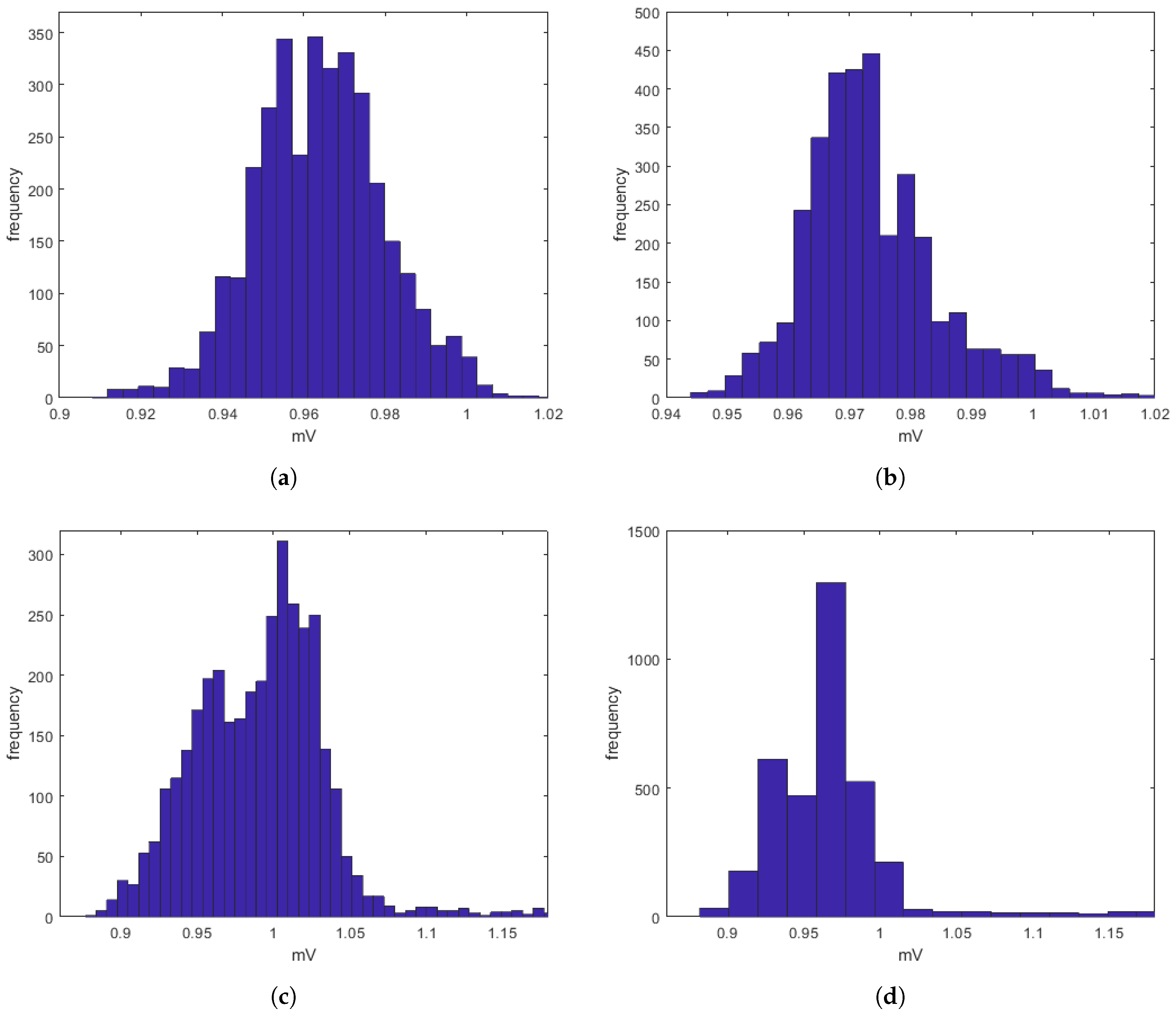
It is worth noting that the $ECG$s concerning a particular pathology are qualitatively similar to each other. This has an impact on the fact that the histograms relating to the similar $ECG$s signals show strong similarities. In parallel, also $ECG$s signals without pathologies are qualitatively similar to each other. Also in this case, the relative histograms are similar. Usually, $ECG$s histograms highlight Gaussian trends as depicted in Figure 11a–d where histograms for typical $ECG$s characterized by normal sinus rhythm, atrial fibrillation, atrial flutter and premature ventricle contraction, respectively, are shown. Therefore, it makes sense to collect $ECG$s characterized by the same pathology in one single class while all the $ECG$s without pathologies can be considered as belonging to a single class. In this way, we obtain four classes of $ECG$s signals: the first class is related to the 140 signals without pathologies (normal sinus rhythm); the second class relates to the 140 signals affected by atrial fibrillation; the third class is related to the 140 $ECG$s that show atrial flutter while the last class, the fourth, collects the 140 $ECG$s, which show premature ventricle contraction.

Thus, it is sufficient to consider mean $m_{ij}$ and standard deviation ${\sigma }_{ij}$ to characterize the ith $ECG$ belonging to the jth. Then, different $ECG$s belonging to the same class highlights light variations of both mean and standard deviation. However, we need to consider just only value for both mean and standard deviation for calculating the Gaussian fuzzy membership function related to the jth class. Therefore, if $K{P}_j$, $j\in \{1,2,3\}$, is the jth class of $ECG$s, it follows that

$${\mu }_{K{P}_j}=\frac{{\sum }_1^{140}{m}_{ij}}{140}$$

(32)

that is the mean value of the means and

$${\sigma }_{K{P}_j}=max\left\{{\sigma }_{ij}\right\}$$

(33)

that is the maximum value of all the standard deviation. Similarly, the same procedure has been applied to the class of $ECG$s without pathologies achieving $m_{NP}$ and ${\sigma }_{NP}$. To build the membership function related to each class $K{P}_j$ and $NP$ we make the relative Gaussian membership functions:

$${\mu }_{K{P}_j}=e^{-\frac{{(x-m_{K{P}_j})}^2}{2{\sigma }_{K{P}_j}^2}}$$

(34)

and

$${\mu }_{NP}=e^{-\frac{{(x-m_{N{P}_j})}^2}{2{\sigma }_{N{P}_j}^2}}.$$

(35)

In this framework, it makes sense to consider the mean of the means of the $ECG$s belonging to each class as the mean value representing that class while, for the standard deviation, we consider the maximum value of all the single standard deviations in order to cover all the $ECG$s belonging to that class.

10.4. Results of Interest

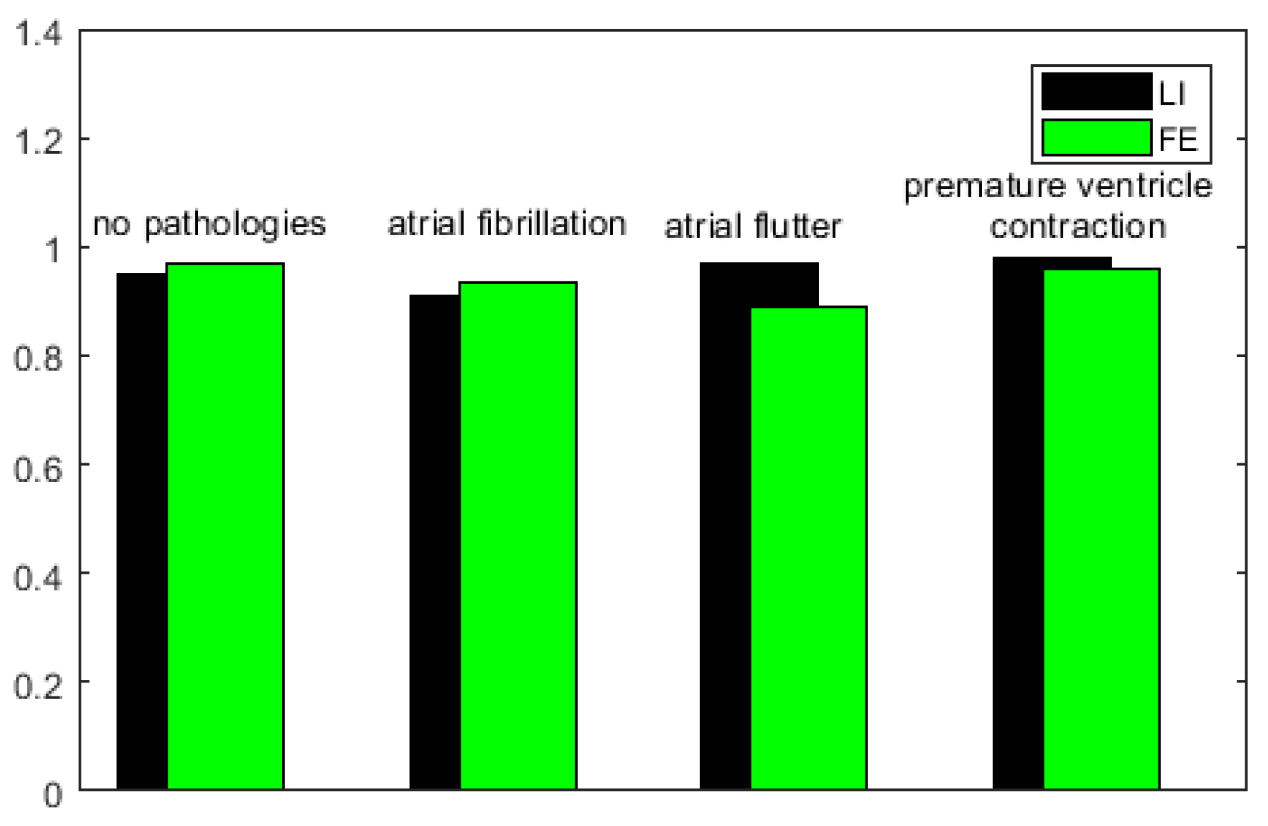
To underline the fuzziness content of each class, both fuzziness indexes ((26) and (27)) for each class were computed: the high values obtained (that is, very close to the unit value) confirmed the high level of fuzziness contained in each class (see Figure 12). In particular, the class of the $ECG$s without pathologies obtained $LI=0.97$ and $FE=0.98$, respectively, while the class of the $ECG$s with atrial fibrillation obtained $LI=0.94$ and $FE=0.95$, respectively. Moreover, concerning the class of the $ECG$s with atrial flutter achieved $LI=0.98$ and $FE=0.92$, respectively. Finally, regarding the class of the $ECG$s with premature ventricle contraction, $LI=0.97$ and $FE=0.97$ were obtained, respectively. This justifies the use of the fuzzy similarity based approach for the analysis of $ECG$s.

Thus, a unique fuzzy membership function for each class has been achieved according to Section 10.3, obtaining four membership functions (the first one related to $ECG$s without heart disease, and the other three related to $ECG$s affected by atrial fibrillation, atrial flutter and premature ventricle contraction, respectively). Therefore, for each $ECG$ numerically obtained by the McSharry dynamical model (Figure 3a,b and Figure 4a) the four fuzzy similarities, $F{S}_1$, $F{S}_2$, $F{S}_3$ and $F{S}_4$, with respect to the four classes of $ECG$s have been computed and the results have been reported in

Table 4. $F{S}_1$, $F{S}_2$, $F{S}_3$ and $F{S}_4$ achieved for $ECG$s related to Case (a).

	Figure 3a	Figure 3b	Figure 4a	Figure 5	Figure 6a	Figure 7a	Figure 8a
no pathologies
$F{S}_1$	0.96	0.99	0.99	0.97	0.12	0.09	0.15
$F{S}_2$	0.94	0.971	0.989	0.98	0.13	0.11	0.14
$F{S}_3$	0.97	0.979	0.987	0.99	0.136	0.12	0.13
$F{S}_4$	0.93	0.73	0.988	0.98	0.134	0.129	0.129
atrial fibrillation
$F{S}_1$	0.14	0.14	0.135	0.01	0.93	0.16	0.09
$F{S}_2$	0.16	0.19	0.139	0.026	0.932	0.151	0.09
$F{S}_3$	0.165	0.196	0.138	0.15	0.921	0.146	0.09
$F{S}_4$	0.17	0.09	0.138	0.165	0.909	0.144	0.08
atrial flutter
$F{S}_1$	0.18	0.16	0.14	0.164	0.14	0.98	0.07
$F{S}_2$	0.16	0.17	0.21	0.163	0.142	0.99	0.11
$F{S}_3$	0.156	0.188	0.16	0.162	0.143	0.985	0.12
$F{S}_4$	0.164	0.15	0.04	0.161	0.145	0.987	0.111
premature ventricle contraction
$F{S}_1$	0.2	0.15	0.159	0.04	0.139	0.04	0.99
$F{S}_2$	0.175	0.14	0.165	0.04	0.132	0.039	0.97
$F{S}_3$	0.161	0.142	0.145	0.048	0.138	0.041	0.98
$F{S}_4$	0.171	0.03	0.161	0.145	0.137	0.04	0.98

respectively, highlighting as Figure 3a,b and Figure 4a belongs to the class of normal $ECG$s (i.e., without heart diseases) due to the high fuzzy similarities obtained. This is supported by the fact that the fuzzy similarities values of Figure 3a,b and Figure 4a obtained with the other classes are far from reaching the unit value as shown in Table 4 (in bold). Similarly, the fuzzy similarities of the $ECG$s obtained with the proposed approach were computed with the representative $ECG$s of each class. Also in these cases the results confirmed the qualitative analysis. In particular, concerning the Case (a), Figure 5 belongs to the class of the $ECG$s of patients without cardiac pathologies because the $F{S}_1$, $F{S}_2$, $F{S}_3$ and $F{S}_4$ values obtained with respect this class are very close to the unit value (in bold), while the values of fiìuzzy similarities obtained with respect to the other classes with pathologies are extremely low (see Table 4). Moreover, Table 4 highlights that $ECG$ depicted in Figure 6a belongs to the class of $ECG$s affected by atrial fibrillation because $F{S}_1$, $F{S}_2$, $F{S}_3$ and $F{S}_4$ values achieved are very close to unity (in bold). Again, Table 4 proves that the $ECG$ shown in Figure 7a belongs to the class of $ECG$s affected by atrial flutter ($F{S}_1$, $F{S}_2$, $F{S}_3$ and $F{S}_4$ are very close to unity) (in bold). Finally, Table 4 puts in evidence that the $ECG$ depicted in Figure 8a belongs to the class of $ECG$s affected by premature ventricle contraction ($F{S}_1$, $F{S}_2$, $F{S}_3$ and $F{S}_4$ are very close to unity) (in bold). Also for Cases (b) and (c) elaborated with the approach proposed in this paper, the quantitative analysis using fuzzy similarities confirmed the qualitative considerations as shown in

Table 5. $F{S}_1$, $F{S}_2$, $F{S}_3$ and $F{S}_4$ achieved for $ECG$s related to Case (b).

	Figure 9a	Figure 9b	Figure 9c	Figure 9d
no pathologies
$F{S}_1$	0.98	0.13	0.12	0.16
$F{S}_2$	0.98	0.144	0.11	0.14
$F{S}_3$	0.96	0.134	0.13	0.12
$F{S}_4$	0.97	0.131	0.14	0.11
atrial fibrillation
$F{S}_1$	0.13	0.96	0.17	0.12
$F{S}_2$	0.133	0.955	0.132	0.11
$F{S}_3$	0.135	0.951	0.144	0.15
$F{S}_4$	0.42	0.92	0.157	0.11
atrial flutter
$F{S}_1$	0.21	0.13	0.99	0.12
$F{S}_2$	0.22	0.11	0.99	0.11
$F{S}_3$	0.21	0.123	0.99	0.13
$F{S}_4$	0.21	0.14	0.97	0.11
premature ventricle contraction
$F{S}_1$	0.21	0.16	0.169	0.99
$F{S}_2$	0.118	0.15	0.166	0.99
$F{S}_3$	0.143	0.144	0.157	0.97
$F{S}_4$	0.124	0.09	0.181	0.968

and

Table 6. $F{S}_1$, $F{S}_2$, $F{S}_3$ and $F{S}_4$ achieved for $ECG$s related to Case (c).

	Figure 10a	Figure 10b	Figure 10c	Figure 10d
no pathologies
$F{S}_1$	0.99	0.13	0.12	0.19
$F{S}_2$	0.98	0.14	0.13	0.17
$F{S}_3$	0.99	0.155	0.132	0.15
$F{S}_4$	0.98	0.159	0.131	0.137
atrial fibrillation
$F{S}_1$	0.12	0.97	0.17	0.11
$F{S}_2$	0.122	0.952	0.17	0.1
$F{S}_3$	0.139	0.93	0.162	0.12
$F{S}_4$	0.169	0.94	0.139	0.13
atrial flutter
$F{S}_1$	0.16	0.15	0.99	0.11
$F{S}_2$	0.156	0.15	0.99	0.21
$F{S}_3$	0.146	0.177	0.984	0.22
$F{S}_4$	0.154	0.12	0.97	0.211
premature ventricle contraction
$F{S}_1$	0.21	0.16	0.162	0.98
$F{S}_2$	0.18	0.144	0.155	0.975
$F{S}_3$	0.169	0.153	0.151	0.99
$F{S}_4$	0.177	0.11	0.119	0.99

, respectively.

11. Conclusions

11.1. Some Considerations on the Stability of the Equilibrium Position

In this paper, we have analyzed in-depth the McSharry model [24]. The dynamic system (5) (a part of the McSharry model (6)) was studied, highlighting the behavior of the single equilibrium position (9), which was found to be unstable (Propositions 1 and 2). This unstable equilibrium position, located at the origin of the coordinate reference system, corresponds to the cusp of the T wave (thought as a strong distortion) of the QRST complex. Furthermore, this unstable equilibrium position corresponds to a point not admitted by the generating equation of the $ECG\left(t\right)$, so that this undesirable instability is, in fact, eliminated.

11.2. On the Uniqueness of the Solution for the McSharry Model and Numerical Approach

Firstly, we observed that the McSharry model depends on the trigonometric function $atan2$ (see (7)), thus that the six specific McSharry systems have been derived, according to the value assumed by $atan2$ (systems (14)–(17), (19) and case (f) in Section 8.6). Furthermore, once that the McSharry model was written in the form (13) as a Cauchy problem and verified that $\underline{h}(t,\chi \left(t\right))$ results in a continuous (Proposition 3) and uniformly Lipschitzian (Proposition 4), we have demonstrated that this modified system admits a unique solution (Theorem 1). We observe that the fact that $\underline{h}(t,\chi \left(t\right))$ is not only continuous but also the Lipschitzian suggests that it has limited growth in the sense that the ratio between the variation of the ordinate and the variation of the abscissa can never exceed a fixed value. Lipschitzianity plays a key role in the uniqueness of solutions in Cauchy problems related to ordinary differential equations. It is, in fact, a condition that guarantees the existence and uniqueness of the solution for a certain initial condition. Also in this case the six models obtained as a function of the different values of $atan2$ admit unique solutions (Theorem 1). However, three of these systems have been discarded as providing solutions that do not adhere to the clinical reality (some terms of the respective solutions cancel out as t increases, see (17)—case (f) in Section 8.6. This is due to the fact that the solutions obtained are functions having terms in the form of negative exponential with a high time constant, so that the transient quickly extinguishes, leaving a term depending on the respiratory artifact. The three remaining systems (14)–(16) have been solved numerically through a procedure based on the four-stage Lobatto IIIa formula implemented in MatLab^® R2017a using the bvp5c subroutine, once the starting problem has been transformed into an equivalent boundary value problem [25,44]. The solutions obtained by solving these three systems, as shown in Figure 3a,b and Figure 4a, show a good regularity of the QRST wave complex comparable with those provided by the McSharry model. In these cases, the regularity of the solutions obtained largely depends on the fact that the respiratory artifact is no longer preponderant (as in the excluded cases) while the effects due to the trigonometric terms in which the arguments depend on the dynamic parameters of the system prevail.

11.3. On the Proposed Approach for Modifying the McSharry Model

The core of this paper is represented by the modification of the McSharry system (5) to simulate $ECG$ affected by cardiac pathologies. These consist in algebraically modifying the system (5) by applying a linear transformation (with numeric parameters $k_1$ and $k_2$) and a rotation function of an angle $\varphi$, as detailed in (20). Obviously, by varying these parameters, different cardiac pathologies can be simulated since by altering these variables we can alter the PQRST complex as well (we point out that, if $k_1=k_2=1$ and $\varphi =0$, the normal sinus rhythm takes place). Three heart diseases have been taken into account: atrial fibrillation, atrial flutter and premature ventricle contraction (as they are the most common heart diseases not associated with specific symptoms and therefore at high risk), in which the parameters $k_1$, $k_2$ and $\varphi$ are specified in Table 3. After verifying that the new system (20) admits the same unstable equilibrium position as (5) (and therefore, as specified above, eliminated) only three cases have been studied (as for the McSharry model (6)) because the remaining three models provide clinically meaningless results. As far as normal sinus rhythm is concerned, all the three considered cases have provided regular trends that can be completely superimposed on $ECG$s taken directly by patients. Once $k_1$ and $k_2$ are set to simulate the presence of atrial fibrillation (see Table 3) the $ECG$ obtained in the three cases considered are shown in the Figure 6a, Figure 9b and Figure 10b, which show how the proposed model is able to reproduce the deformation of the QRST complex related to this pathology. In these cases, according to the $ECG$ traces taken directly on patients affected by atrial fibrillation, an increase in heart rate and an irregular R-R rhythm (at variable distances) are highlighted. The QRS complex appears narrow while the P waves are almost absent and replaced by waves with a different morphology from each other. The P-QRS ratio is not valuable. By setting $k_1$, $k_2$ and $\varphi$ to simulate the atrial flutter (see Table 3), for the three cases studied, the traces are displayed in Figure 7a, Figure 9c and Figure 10c. Also in these cases, in adherence to the typical clinical $ECG$ detected directly on patients, reliable results are obtained as the obtained $ECG$ trends show a continuous and regular atrial activation with a saw-tooth pattern, evident in the lower leads. Finally, by setting $k_1$, $k_2$ and $\varphi$ to simulate premature ventricle contraction, Figure 8a, Figure 9d and Figure 10d show, as clinically expected, large QRS complexes, not preceded by the P wave and therefore clearly distinguishable from sinus ones. In this case, retro activation of the atria may or may not occur. The qualitative analysis was also confirmed from the quantitative point of view. In particular, since the $ECG$s are often affected by uncertainty and/or imprecision due to various types of artifacts (such as breathing, incorrect application of the electrodes), they take on an evident fuzzy connotation and therefore need to be treated in the fuzzy domain. Once the fuzziness content of each $ECG$ has been highlighted using two specific indices formulated in (26) and (27) respectively (in the sense that the high values obtained showed a high content of fuzziness in each signal), this qualitative analysis was quantitatively confirmed through the computation of particular four indices of fuzzy similarities, $F{S}_1$, $F{S}_2$ $F{S}_3$ and $F{S}_4$ as formulated in (28)–(31) respectively. Each $ECG$ obtained was compared to four classes of $ECG$s obtained directly on patients (one class for $ECG$ without pathologies, three classes for the three pathologies chosen, respectively). Where it is not possible to directly observe the pathology form a direct qualitative analysis of the $ECG$, the procedure proposed registers the presence of a pathology (far from the fuzzy similarities unitary value) without classifying the type of the pathology because the fuzzy similarity values are dissimilar to the one typical of each class. Moreover, the classification puts in evidence that the detection of the presence of pathologies in an $ECG$ is marked by comparing the same $ECG$ with a benchmark (that is, an $ECG$ without pathologies). In addition, each detection (for each class of pathology) presents ranges of possible values for fuzzy similarities, so that, by comparison, the kind of pathology can be deduced. The results obtained confirm the good quality of the proposed procedure. Specifically, in terms of detection, the system is able to record the presence of a pathology in an $ECG$ so that the proposed method can be considered to all intents and purposes a classification system of cardiac pathologies present in $ECG$s If the system detects the presence of a cardiac anomaly in an $ECG$ without, however, classifying it, it is possible to create an additional class of pathologies that do not fall into those considered. From the analysis of the results obtained, we deduce that the approach proposed in this paper for the generalization of the McSharry model presented in [24], appears valid in simulating certain cardiac pathologies, highlighting $ECG$s that are completely consistent with a real clinic. Moreover, the results obtained are encouraging as they emphasize the capacity to develop a database of pathological $ECG$ signals with a sufficient level of differentiation as the pathology changes. In addition, the fuzzy similarity approach obtains relevant results in terms of detection and classification of pathologies in $ECG$s. Being the procedure characterized by a low computational complexity, it is easy to design a hardware system able to perform the classification really useful for real-time applications. Furthermore, uncertainty and imprecision are well highlighted by computation of suitable indexes of fuzziness and the proposed approach does not require pre-processing of the $ECG$s because the procedure works well on raw data.

12. Future Perspectives

However, there is no doubt that any heart disease presents, from a clinical point of view, different levels of severity. Therefore, in the future, it will be desirable to take this important aspect into account by generalizing the proposed procedure in order to simulate $ECG$ with pathologies of different severity levels. Finally, since the $ECG$ is affected by numerous artifacts (not only due to breathing but also, for example, to the incorrect positioning of the electrodes on the skin), it will be desirable, to integrate the model with terms that take into account such eventualities.

References

1. Hampton, J. The ECG Made Easy; Elsevier: London, UK; New York, NY, USA; Oxford, UK; Philadelphia, PA, USA, 2019. [Google Scholar]
2. Gargiulo, G.D.; Bifulco, P.; Cesarelli, M.; McEwan, A.L.; Moeinzadeh, H.; O’Loughlin, A.; Shugman, I.M.; Tapson, J.; Thiagalingam, A. On the Einthoven Triangle: A Critical Analysis of the Single Rotating Dipole Hypothesis. Sensors 2018, 18, 2353. [Google Scholar]
3. Labatin, R.D.; Munoz, E.; Piuri, V.; Sassi, R.; Scotti, F. Deep-ECG: Convolutional Neural Newtorks for ECG biometric Recognition. Pattern Recognit. Lett. 2019, 20, 168–181. [Google Scholar]
4. Biglu, M.H.; Ghavami, M.; Biglu, S. Cardiovascular Diseases in the Mirror of Science. J. Cardiovasc. Thorac. Res. 2016, 8, 158–163. [Google Scholar] [PubMed] [Green Version]
5. La Foresta, F.; Morabito, F.C.; Azzerboni, B.; Ipsale, M. PCA and ICA for the extraction of EEG dominant components in cerebral death assessment. Proc. Int. Jt. Conf. Neural Netw. 2005, 4, 32532–32537. [Google Scholar]
6. La Foresta, F.; Mammone, N.; Morabito, F.C. Independent component and wavelet analysis for ECG extraction: The ST waveform evaluation. In Proceedings of the 2005 IEEE International Conference on Computational Intelligence for Measurement Systems and Applications, Messina, Italy, 20–22 July 2005; pp. 86–90. [Google Scholar]
7. Alqudah, A.M.; Albadarneh, A.; Abu-Qasmieh, I.; Alquran, H. Developing of Robust and High Accurate ECG Beat Classification by Combining Gaussian Mixture s and Wavelets Features. Australas. Phys. Eng. Sci. Med. 2019, 42, 149–157. [Google Scholar]
8. Attia, Z.I.; DeSimone, C.V.; Dillon, J.J.; Sapir, Y.; Somers, V.K.; Dugan, J.L.; Bruce, C.J.; Ackerman, M.J.; Asirvatham, S.J.; Striemer, B.L.; et al. Novel Bloodless Potassium Determination Using a Signal-Processed Single-Lead ECG. J. Am. Heart Assoc. 2016. [Google Scholar] [CrossRef] [Green Version]
9. Němcová, A.; Smíšek, R.; Maršánová, L.; Smital, L.; Vítek, M. A Comparative Analysis of Methods for Evaluation of ECG Signal Quality after Compression. BioMed Res. Int. 2018, 2018, 1–26. [Google Scholar]
10. Stauffer, F.; Thielen, M.; Sauter, C.; Chardonnens, S.; Bachmann, S.; Tybrandt, K.; Peters, C.; Hierold, C.; Vörös, J. Skin Conformal Polymer Electrodes for Clinical ECG and EEG Recording. Adv. Healthc. Mater. 2018, 12, 422–441. [Google Scholar]
11. Manikandan, M.S.; Dandapat, S. Wavelet Energy Based Diagnostic Distortion Measure for ECG. Biomed. Signal Process. Control 2007, 2, 80–96. [Google Scholar]
12. Strodthoff, N.; Strdothoff, C. Detecting and Interpreting Myocardial Infarction Using Fully Convolutional Neural Networks. Physiol. Meas. 2019, 40, 015001. [Google Scholar]
13. Selder, J.L.; Breukel, L.; Block, S.; van Rossum, A.C.; Tulevski, I.I.; Allaart, C.P. A Mobile One-Lead ECG Device Incorporated in a Symptom-Driven Remote Arrhythmia Monitoring Programm. The First 5982 Hartwacht ECGs. Neth. Hearth J. 2019, 27, 38–45. [Google Scholar]
14. Tabassum, T.; Ahmed, M. A Simplified Cardiac Conduction Model and Twelve-Lead ECG Generation. In Proceedings of the IEEE International Conference on Computer, Electrical & Comunication Engineering (ICCECE), Kolkata, India, 17–18 January 2020; pp. 1–5. [Google Scholar]
15. Hernandez-Caceres, J.L.; Gonzales-Fernandez, R.; Ontivero-Ortega, M.; Molte, G. Introducing BisQ, A Bicoherence-Based Nonlinear Index to Explore the Heart Rhythm. Math. Comput. Appl. 2020, 25, 45. [Google Scholar]
16. Trayanova, N.A. Whole Heart Modeling: Applications to Cardiac Electrophysiology and Electromechanics. Circ. Res. 2012, 108, 113–128. [Google Scholar]
17. Vinciguerra, V.; Ambra, E.; Maddiona, L.; Romeo, M.; Mazzillo, M.; Rundo, F.; Fallica, G.; Pompeo, F.; Chiarelli, A.M.; Zappasodi, F.; et al. PPG/ECG Multisite Combo System Based on SiPM Technology. In CNS 2018. Lecture Notes in Electrical Engineering; Springer: Cham, Switzerland, 2018; p. 53. [Google Scholar]
18. Quiroz-Juárez, M.A.; Jiménez-Ramírez, O.; Vázquez-Medina, R.; Brena-Medina, V.F.; Aragón, J.L.; Barrio, R.A. Generation of ECG Signals from a Reaction-Diffusion Model Spatially Discretized. Sci. Rep. 2019, 9. [Google Scholar] [CrossRef] [Green Version]
19. Sornmo, L.; Laguna, P. Electrocardiogram (ECG) Signal Processing. In Wiley Encyclopedia of Biomedical Engineering; Wiley: New York, NY, USA, 2006. [Google Scholar]
20. Rai, H.M.; Trivedi, A.; Shukla, S. ECG Signal Processing for Abnormalities Detection Using Multi-Resolution Wavelet Transform and Artificial Neural Newtork Classifier. Measurement 2013, 46, 3238–3246. [Google Scholar]
21. Gacek, A. An Introduction to ECG Signal Processing and Analysis; Gacek, A., Pedrycz, W., Eds.; Springer: London, UK, 2012; pp. 21–46. [Google Scholar]
22. Jaros, R.; Martinek, R.; Kahankova, R. Non-Adaptive Methods for Fetal ECG Signal Processing: A Review and Appraisal. Sensors 2018, 18, 3648. [Google Scholar]
23. Sameni, R.; Clifford, G.D. A Review of Fetal ECG Signal Processing: Issues and Promising Directions. Open Spacing Electrophysiol. Ther. J. 2010, 1, 4–20. [Google Scholar]
24. McSharry, P.E.; Clifford, G.D.; Tarassenk, L.; Smith, L.A. A Dynamical Model for Generating Synthetic Electrocardiogram Signals. IEEE Trans. Biomed. Eng. 2003, 50, 289–294. [Google Scholar]
25. Quarteroni, A.; Sacco, R.; Saleri, F. Numerical Mathematics; Springer: Berlin/Heidelberg, Germany, 2007. [Google Scholar]
26. Sayadi, O.; Mohammad, B.S.; Gari, D.C. Synthetic ECG generation and Bayesian filtering using a Gaussian wave-based dynamical model. Physiol. Meas. 2010, 31, 1309. [Google Scholar]
27. Jackson, S.; Cogswell, M.E.; Zhao, L.; Terry, A.L.; Wang, C.Y.; Wright, J.; King, S.M.C.; Bowman, B.; Chen, T.-C.; Merritt, R.; et al. Association Between Urinary Sodium and Potassium Excretion and Blood Pressure Among Adults ioon the United States, National Health and Nutrition Examination Survey. Circulation 2018, 137, 237–246. [Google Scholar]
28. Aaron, K.J.; Sanders, P.W. Role of Dietary Salt and Potassium Intake in Cardiovascular Health and Disease: A Review of the Evidence. Mayo Clin. Proc. 2014, 11, 9. [Google Scholar]
29. Vicente, J.; Zusterzeel, R.; Johannesen, L.; Ochoa-Jimenez, R.; Mason, J.W.; Sanabria, C.; Kemp, S.; Sager, P.T.; Patel, V.; Matta, M.K.; et al. Assessment of Multi-Ion Channel Block in a Phase I Randomized Study Design: Results of the CiPA Phase I ECG Biomarker Validation Study. Clin. Pharmacol. Ther. 2018, 105, 111–129. [Google Scholar]
30. Garcia, M.D.; Tomas, B. 12 Lead ECG: The Art of Interpretation; Pearson: London, UK, 2014. [Google Scholar]
31. Goldberger, A.L.; Goldberger, Z.D.; Shvilkin, A. Goldberger’s Clinical Electrocardiography; Elsevier: Amsterdam, The Netherlands, 2017. [Google Scholar]
32. Versaci, M. Soft Computing Approach to Predict Intracranial Pressure Values. Am. J. Appl. Sci. 2014, 11, 844–850. [Google Scholar]
33. Versaci, M.; Morabito, F.C. Fuzzy Time Series Approach for Disruption Prediction in Tokamak Reactors. IEEE Trans. Magn. 2003, 39, 1503–1506. [Google Scholar]
34. Cacciola, M.; La Foresta, F.; Morabito, F.C.; Versaci, M. Advanced Use of Soft Computing and Eddy Current Test to Evaluate Mechanical Integrity of Metallic Plates. NdT E Int. 2007, 40, 357–362. [Google Scholar]
35. Angiulli, G.; Jannelli, A.; Morabito, F.C.; Versaci, M. Reconstructing the Membrane Detection of a 1D Electrostatic-Driven MEMS Device by the Shooting Method: Convergence Analysis and Ghost Solutions Identification. Comput. Appl. Math. 2018, 37, 4484–4498. [Google Scholar]
36. Schmidt, R.F.; Thews, G. Human Physiology; Springer: Berlin/Heidelberg, Germany, 1989. [Google Scholar]
37. Agarwal, A.M. Trigonometry; Arihant: Delhi, India, 2018. [Google Scholar]
38. Barreira, L.; Valls, C. Dynamical Systems; Springer: London, UK, 2013. [Google Scholar]
39. Cacciola, M.; Calcagno, S.; Morabito, F.C.; Versaci, M. Swarm Optimization for Imaging of Corrosion by Impedance Measurements in Eddy Current Tests. IEEE Trans. Magn. 2007, 43, 1853–1856. [Google Scholar]
40. Cacciola, M.; Pellicanó, D.; Megali, G.; Lay-Ekuakille, A.; Versaci, M.; Morabito, F.C. Aspects About Air Pollution Prediction on Urban Environment. In Proceedings of the 4th IMEKO TC19 Symposium on Environmental Instrumentation and Measurements 2013: Protection Environment, Climate Changes and Pollution Control, Lecce, Italy, 3–4 June 2013; pp. 15–20. [Google Scholar]
41. Coletti, G.; Bouchon-Meunier, B. Fuzzy Similarity Measures and Measurement Theory. In Proceedings of the 2019 IEEE International Conference on Fuzzy Systems (FUZZ-IEEE), New Orleans, LA, USA, 23–26 June 2019; pp. 1–8. [Google Scholar]
42. Moody, G.B.; Mark, R.G. The impact of the MIT-BIH Arrhythmia Database. IEEE Eng. Med. Biol. 2001, 20, 45–50. [Google Scholar]
43. Goldberger, A.L.; Amaral, L.A.N.; Glass, L.; Hausdorff, J.M.; Ivanov, P.C.; Mark, R.G.; Mietus, J.E.; Moody, G.B.; Peng, C.-K.; Stanley, H.E. PhysioBank, PhysioToolkit, and PhysioNet: Components of a new research resource for complex physiologic signals. Circulation 2000, 101, e215–e220. [Google Scholar]
44. Iserles, A. A First Course in the Numerical Analysis of Differential Equations; Cambridge University Press: Cambridge, UK, 2009. [Google Scholar]
Figure 1. (a) Sagittal plane ( x z plane), frontal plane ( y z plane) and transverse plane ( x y plane) (public domain image). (b) Typical E C G signals: continuous line represents a normal E C G . Dotted and dashed lines represent pathological E C G s.
Computation 08 00092 g001
Figure 2. (a) A typical vector cardiogram (VCG) loop for a normal cardiac cycle. (b) A typical VCG loop characterized by a nodal rhythm disease.
Computation 08 00092 g002
Figure 3. E C G reconstruction by (a) System (14) (case (a)) and (b) System (15) (case (b)).
Computation 08 00092 g003
Figure 4. (a) E C G reconstruction by system (16) (case (c)). (b) Typical E C G obtained from a patient not suffering from any cardiac disease.
Computation 08 00092 g004
Figure 5. Case (a) of the proposed methodology: normal sinus rhythm.
Computation 08 00092 g005
Figure 6. Case (a) of the proposed methodology: (a) atrial fibrillation and (b) typical E C G with atrial fibrillation.
Computation 08 00092 g006
Figure 7. Case (a) of the proposed methodology: (a) atrial flutter and (b) typical E C G with atrial flutter.
Computation 08 00092 g007
Figure 8. Case (a) of the proposed methodology: (a) premature ventricle contraction and (b) typical E C G with premature ventricle contraction.
Computation 08 00092 g008
Figure 9. Case (b) of the proposed methodology: (a) normal sinus rhythm (b) atrial fibrillation (c) atrial flutter (d) premature ventricle contraction.
Computation 08 00092 g009
Figure 10. Case (c) of the proposed methodology: (a) normal sinus rhythm (b) atrial fibrillation (c) atrial flutter (d) premature ventricle contraction.
Computation 08 00092 g010
Figure 11. Histograms for typical E C G s characterized by (a) normal sinus rhythm, (b) atrial fibrillation, (c) atrial flutter, (d) premature ventricle contraction.
Computation 08 00092 g011
Figure 12. Evaluation of linear index (LI) and fuzzy entropy (FE) for each category of E C G s.
Computation 08 00092 g012