Colebrook’s Flow Friction Explicit Approximations Based on Fixed-Point Iterative Cycles and Symbolic Regression

Abstract

The logarithmic Colebrook flow friction equation is implicitly given in respect to an unknown flow friction factor. Traditionally, an explicit approximation of the Colebrook equation requires evaluation of computationally demanding transcendental functions, such as logarithmic, exponential, non-integer power, Lambert W and Wright Ω functions. Conversely, we herein present several computationally cheap explicit approximations of the Colebrook equation that require only one logarithmic function in the initial stage, whilst for the remaining iterations the cheap Padé approximant of the first order is used instead. Moreover, symbolic regression was used for the development of a novel starting point, which significantly reduces the error of internal iterations compared with the fixed value staring point. Despite the starting point using a simple rational function, it reduces the relative error of the approximation with one internal cycle from 1.81% to 0.156% (i.e., by a factor of 11.6), whereas the relative error of the approximation with two internal cycles is reduced from 0.317% to 0.0259% (i.e., by a factor of 12.24). This error analysis uses a sample with 2 million quasi-Monte Carlo points and the Sobol sequence.

1. Introduction

The Colebrook equation, Equation (1) [1], is implicitly given in respect to the unknown flow friction factor $f$, which is captured implicitly in a logarithmic expression in a way that can be expressed explicitly only using special functions such as the Lambert W function or its cognate Wright Ω [2,3,4,5,6,7,8,9]. In the latter instance, the Colebrook equation can be solved only numerically using iterative procedures [10] or using specially developed explicit approximations [11,12,13,14,15].

$$\frac{1}{\sqrt{f}}=-2·{\log }_{10}\left(\frac{2.51}{\mathit{Re}}·\frac{1}{\sqrt{f}}+\frac{\epsilon }{3.71}\right),$$

(1)

where f is the Darcy flow friction factor (dimensionless), Re is the Reynolds number (dimensionless) and ε is the relative roughness of inner pipe surface (dimensionless).

The Colebrook equation has been known since the end of the 1930s and is based on an experiment by Colebrook and White [16] that had been performed a few years earlier using pipes with different inner surface roughness, from smooth to very rough. As the Colebrook equation is empirical [1,16], its accuracy can be disputed [17,18] (e.g., the new Oregon and Princeton experiment related to pipe friction [18]); nevertheless, the equation is widely accepted as a standard and is in common use in the design of water and gas pipe networks [19]. It can be also adapted for special cases such as air flow through fuel cells [20], water flow in rivers [21,22] and blood flow in blood vessels [23].

Praks and Brkić [24] recently showed a Newton–Raphson iterative solution of the Colebrook equation based on Padé approximants [25,26,27,28,29]. Based on their solution, one simplified approach and a novel starting point that significantly reduces numerical error will be offered herein.

The simplified method is based on the fixed-point method, a variant of the Newton–Raphson method in which the first derivative of the unknown function is equalized to 1 [30]. In the worst case, the demonstrated iterative procedures need up to seven iterations to reach the final accurate solution [10], whereas in this study the explicit approximations derived from the iterative procedure will have relative errors of up to 1.81% and 0.317% in the case of one internal and two internal iterative steps, respectively. Moreover, when the novel simple rational function $p_0$ of Equation (2) is used as a starting point, the relative errors are significantly reduced to 0.156% and 0.0259%, respectively. Such small values of the relative error are acceptable for engineering applications, given the empirical nature of the Colebrook equation [17,18].

The approach with Padé approximants offers an iterative procedure in which the repetition of the computationally expensive logarithmic function is avoided [24]. Using only one logarithmic function together with simple rational functions and avoiding computationally expensive functions, such as exponential functions or functions with non-integer powers, the presented method saves the processor time [7,8,9,12,13,14], which is essential for effective simulations of large pipe networks [19].

The presented approximations are in a form suitable for computer codes and for application in software packages for everyday engineering use.

2. A Fixed-Point Iterative Procedure Based on Padé Approximants

The logarithmic function can be accurately approximated in a certain relatively narrow domain using Padé approximants (an approximation of the given function by a rational function of given order) [24]. For example, ${\log }_{10}\left(97\right)$ can be cheaply approximated knowing that ${\log }_{10}\left(100\right)=2$, and using the fact that ${\log }_{10}\left(97\right)={\log }_{10}\left(\frac{100}{\frac{100}{97}}\right)={\log }_{10}\left(100\right)-{\log }_{10}\left(\frac{100}{97}\right)$, where $\frac{100}{97}\approx 1.0309$, which is close to 1. Consequently, ${\log }_{10}\left(1.0309\right)$ can be accurately estimated by its Padé approximant at the expansion point $x=1$. This simple idea can be used for solving the logarithmic-based Colebrook equation. Starting from the initial point $x_0=\frac{1}{\sqrt{f_0}}\to y_0=\frac{2.51·x_0}{\mathit{Re}}+\frac{\epsilon }{3.71}$, the next value can be calculated as $x_1=-2·{\log }_{10}\left(y_0\right)$. The pre-computed numerical value $\zeta$; $\zeta ={\log }_{10}\left(y_0\right)$ should be used in all the following iterations [24]. The next value $y_1=\frac{2.51·x_1}{\mathit{Re}}+\frac{\epsilon }{3.71}$ and the previous value $y_0$ should be used as the argument of the Padé approximant $z_{01}=\frac{y_0}{y_1}$, where the chosen Padé approximant is $p_{01}=\frac{z_{01}·\left(z_{01}+4\right)-5}{4·z_{01}+2}$. Now, the new value ${\log }_{10}\left(y_1\right)=\zeta +0.8686·p_{01}$ should be used for the calculation $x_1=-2·\zeta +0.8686·p_{01}$ where $0.8686\approx \frac{2}{\ln \left(10\right)}$.

To solve the Colebrook equation using a numerical fixed-point iterative procedure, the steps shown in Figure 1 should be followed. Figure 1 includes a simplified procedure compared with [24], where the Newton–Raphson iterative procedure is used instead of the herein presented fixed-point iterative procedure.

The initial starting point $x_0=\frac{1}{\sqrt{f_0}}$ should be chosen from the domain of applicability of the Colebrook equation, which is $0<\epsilon <0.05$ and $4000<\mathit{Re}<{10}^8$. Every initial starting point chosen from this domain will be suitable, but to reduce the required number of iterations, different strategies are offered [10]. We will demonstrate the approach with the fixed-value initial starting point, but also the approach with the starting point given by the rational function:

$$\begin{array}{cc}\hfill p_0=x_0=\frac{1}{\sqrt{f_0}}=& \frac{2600·\mathit{Re}}{657.7·\mathit{Re}+214600·\mathit{Re}·\epsilon +12970000}-13.58·\epsilon \hfill \\ & +\frac{0.0001165·\mathit{Re}}{0.00002536·\mathit{Re}+\mathit{Re}·\epsilon +105.5}+4.227\hfill \end{array}$$

(2)

Equation (2) was found using the symbolic regression tool Eureqa [31,32] following the approach of Gholamy and Kreinovich [33], in which existing absolute error minimizing software was used to minimize the relative error (various artificial intelligence tools have been used recently for the Colebrook equation, such as symbolic regression [34], novel artificial bee colony programming (ABCP) methods [35], artificial neural networks [36], genetic algorithms [37], etc.). The novel starting point given by Equation (2) has a maximal relative error of only 6.7%, whereas the previous version of the starting point [34] had a maximal relative error of 40%. Thus, we can observe that the approach Gholamy and Kreinovich [33] used was very useful for symbolic regression of the Colebrook equation.

Calculation of ${\log }_{10}\left(y_0\right)$ should not be repeated in each iteration, but its numerical value $\zeta$ should be used in a combination with the Padé approximant in every iteration (with the exception of the first) [24].

Instead of $z_{01}=\frac{y_0}{y_1}$, $z_{02}=\frac{y_0}{y_2}$, $z_{03}=\frac{y_0}{y_3}$, and so on, the adapted chain can be used as $z_{01}=\frac{y_0}{y_1}$, $z_{12}=\frac{y_1}{y_2}$, $z_{23}=\frac{y_2}{y_3}$, etc. [24].

The Padé approximant $\frac{z_{01}·\left(z_{01}+4\right)-5}{4·z_{01}+2}$ used is of the order /1,1/, referring to the polynomial order in the numerator and in the denominator, respectively [24]. As the expansion point $z=1$ is the root of $\ln \left(z\right)$, the accuracy of the Padé approximant decreases. For this reason, setting the OrderMode option in the Matlab Padé command to relative compensates for the decreased accuracy. Consequently, the numerator of the Padé approximant of the order /1,1/ includes the polynomial of the second order.

Possible software implementation of developed algorithms is summarized in Section 4.

3. Explicit Approximations Based on Padé Approximants

Two explicit approximations of the Colebrook equation based on the algorithm from Figure 1 will be shown here. The approximation with one internal iterative cycle will be shown in Section 3.1, while the approximation with two internal iterative cycles will be presented in Section 3.2. The iterative procedures are sensitive, depending on the chosen initial starting point [38], and therefore carefully conducted numerical tests are provided separately for the approximation with one and two internal iterative cycles. In both cases, fixed numerical values for the initial starting points are chosen in such a way as to reduce the final maximal relative error over the domain of applicability of the Colebrook equation. Alternatively, the novel rational function, Equation (2), is used as the initial starting point. We show that this alternative approach significantly reduces the relative error of approximations.

In order to perform a deeper analysis of the turbulent flow, the emphasis of this section is on the Reynolds number $Re$ between 10⁴ and 10⁸ (the analysis is compatible with [39]). However, the error aggregates in the zone between 4000 and 10⁴, where it is still possible that a laminar flow can exist.

3.1. Explicit Approximations with One Internal Iterative Cycle

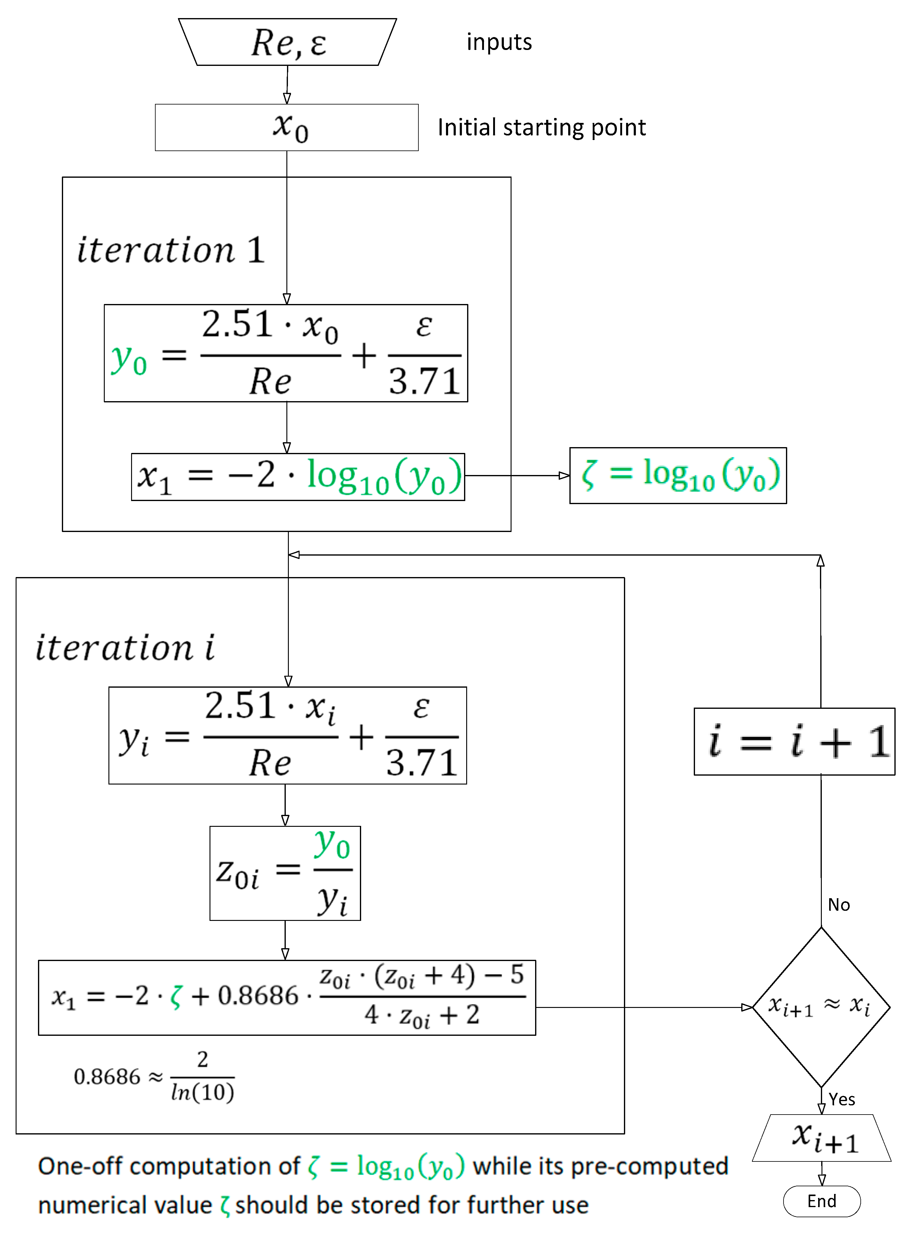
3.1.1. An Explicit Approximation with One Internal Iterative Cycle and a Numerical Fix-Value Starting Point

After numerous numerical tests, it is clear that the algorithm from Figure 1 gives the smallest relative error in the domain of applicability of the Colebrook equation for the approximation with one internal cycle, Equation (3), if the initial starting point is set as $f_0=0.022058\to x_0=\frac{1}{\sqrt{f_0}}=6.73306$ (the numerical value 16.9 of the parameter c in Equation (3) is computed as 2.51 × 6.73306). The maximal relative error of Equation (3) is up to 0.79% and its distribution can be seen in Figure 2.

$$\begin{array}{c}\frac{1}{\sqrt{f}}\approx b+0.8686·\frac{a·\left(a+4\right)-5}{4·a+2}\\ a=\frac{c}{\frac{\epsilon }{3.71}+\frac{2.51·b}{\mathit{Re}}}\\ \begin{array}{c}b=-2·{\log }_{10}\left(c\right)\\ c=\frac{16.9}{\mathit{Re}}+\frac{\epsilon }{3.71}\end{array}\end{array}\},$$

(3)

3.1.2. An Explicit Approximation with One Internal Iterative Cycle and a Starting Point Given by a Rational Function

Using the rational function $p_0$, Equation (2) for the initial starting point $x_0$ and the proposed approximation, Equation (4) has a maximal relative error of 0.101%. The distribution of its relative error is shown in Figure 3. In comparison with the fixed point version, Equation (3)—the novel staring point—Equation (2) reduces the maximal relative error for one internal iterative cycle by a factor of 7.82 (=0.79%/0.101%).

$$\begin{array}{c}\frac{1}{\sqrt{f}}\approx b+0.8686·\frac{a·\left(a+4\right)-5}{4·a+2}\\ a=\frac{c}{\frac{\epsilon }{3.71}+\frac{2.51·b}{\mathit{Re}}}\\ \begin{array}{c}b=-2·{\log }_{10}\left(c\right)\\ c=\frac{2.51·p_o}{\mathit{Re}}+\frac{\epsilon }{3.71}\end{array}\end{array}\},$$

(4)

where $p_o$ is from Equation (2).

3.2. Explicit Approximations with Two Internal Iterative Cycles

3.2.1. An Explicit Approximation with Two Internal Iterative Cycles and a Fixed Starting Point

The explicit approximation of the Colebrook formula with two internal iterative cycles is given in Equation (5). The numerical fixed value 18.15 of the parameter $c$ of Equation (5) depends on the initial starting point, which is carefully chosen to reduce the maximal relative error and corresponds to the initial starting point set as $f_0=0.01912468\to x_0=\frac{1}{\sqrt{f_0}}=7.2310756,$ where $18.15\approx 2.51\times 7.2310756.$ The maximal relative error of Equation (5) is up to 0.172% and its distribution is shown in Figure 4.

$$\begin{array}{c}\frac{1}{\sqrt{f}}\approx b+0.8686·\frac{d·\left(d+4\right)-5}{4·d+2}\\ a=\frac{c}{\frac{\epsilon }{3.71}+\frac{2.51·b}{\mathit{Re}}}\\ \begin{array}{c}b=-2·{\log }_{10}\left(c\right)\\ \begin{array}{c}c=\frac{18.15}{\mathit{Re}}+\frac{\epsilon }{3.71}\\ d=\frac{c}{\frac{\epsilon }{3.71}+\frac{2.51}{\mathit{Re}}·(b+0.8686·\frac{a·(a+4)-5}{4·a+2})}\end{array}\end{array}\end{array}\},$$

(5)

3.2.2. An Explicit Approximation with Two Internal Iterative Cycles and a Starting Point Given by a Rational Function

The introduction of a starting point given by the rational function Equation (2) instead of a fixed point significantly reduces the relative error from 0.172% in Equation (5) to no more than 0.0154% in Equation 6 (i.e., by a factor of 11.16). Equation (6) presents the new explicit approximation with two internal iterative cycles and a starting point given by the rational function, Equation (2), while the distribution of its relative error is shown in Figure 5.

$$\begin{array}{c}\frac{1}{\sqrt{f}}\approx b+0.8686·\frac{d·\left(d+4\right)-5}{4·d+2}\\ a=\frac{c}{\frac{\epsilon }{3.71}+\frac{2.51·b}{\mathit{Re}}}\\ \begin{array}{c}b=-2·{\log }_{10}\left(c\right)\\ \begin{array}{c}c=\frac{2.51·p_o}{\mathit{Re}}+\frac{\epsilon }{3.71}\\ d=\frac{c}{\frac{\epsilon }{3.71}+\frac{2.51}{\mathit{Re}}·\left(b+0.8686·\frac{a·\left(a+4\right)-5}{4·a+2}\right)}\end{array}\end{array}\end{array}\},$$

(6)

where p_o is from Equation (2).

3.3. Further Error Analysis and Comparisons

Table 1. Comparison of maximal relative error (in %) for the first and second iteration without the Padé approximant and with a Padé approximant of the order /1,1/ for the Reynolds number Re from 4000 to 10⁸.

Padé Approximant	No		/1,1/
solution version 1	x = x1 + 0.8686*log(z)		x = x1 + 0.8686*(z*(z + 4) − 5)/(4*z + 2)
Iteration	1	2	1	2
Fixed starting point	1.81%	−0.317%	1.81%	−0.317%
Starting point by Equation (2)	−0.156%	0.0259%	−0.156%	0.0259%

¹ Notation from Matlab codes from Section 4; symbol log(z) of the solution update represents the natural logarithm; both Matlab and MS Excel codes are mathematically equivalent: they use the same function, the natural logarithm. In MS Excel, the natural logarithm is expressed by the symbol ln(x), whereas in Matlab, the natural logarithm is expressed by the symbol log(x).

summarize the results of error analysis for 2 million quasi Monte-Carlo points using the Sobol sequence [40,41] related to Equations (3)–(6). The domain for this analysis in respect to the Reynolds number $\mathit{Re}$ is from 4000 to 10⁸, while for the sample of 740 points, which was used for Figure 2, Figure 3, Figure 4 and Figure 5, the domain is from 10⁴ to 10⁸.

Table 1 shows that iterations using the Padé approximant of the first order /1,1/ ln11(z) = (z*(z + 4) − 5)/(4*z + 2) have the same relative error as iterations using the natural logarithm. For the method with one internal cycle (denoted as Iteration 1 in Table 1), the maximal relative error is approximately 1.81% or 0.156%, whereas for the method with two internal cycles (denoted as Iteration 2 in Table 1), the maximal relative error is only 0.317% or 0.0259%. This analysis also shows that the novel starting point given with Equation (2) is very useful.

Compared with analysis performed in MS Excel where 740 points are used, analysis with 2 million quasi Monte-Carlo points using the Sobol sequence detected additional peaks of error, as shown in

Table 2. Analysis of error performed in MS Excel with 740 points compared with analysis from Matlab with 2 million Monte Carlo samples using the Sobol sequence.

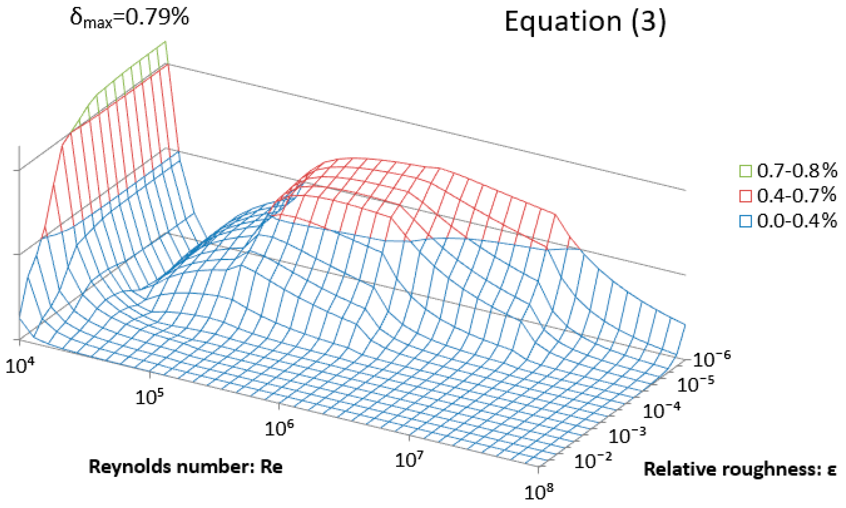
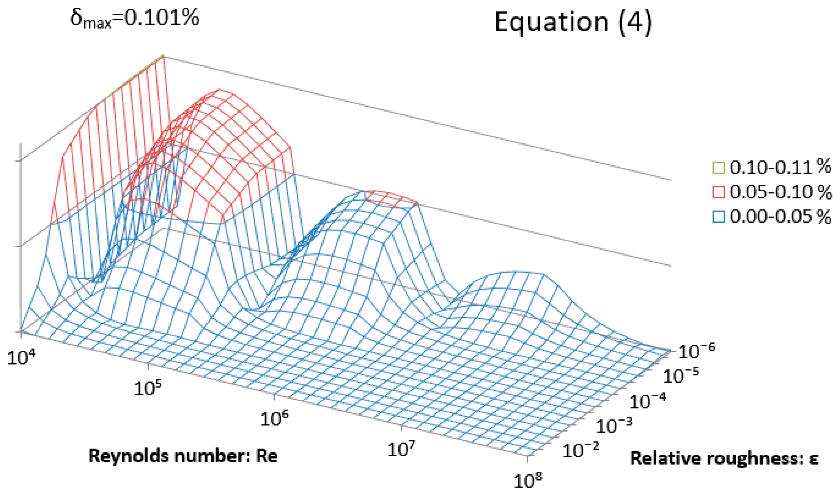
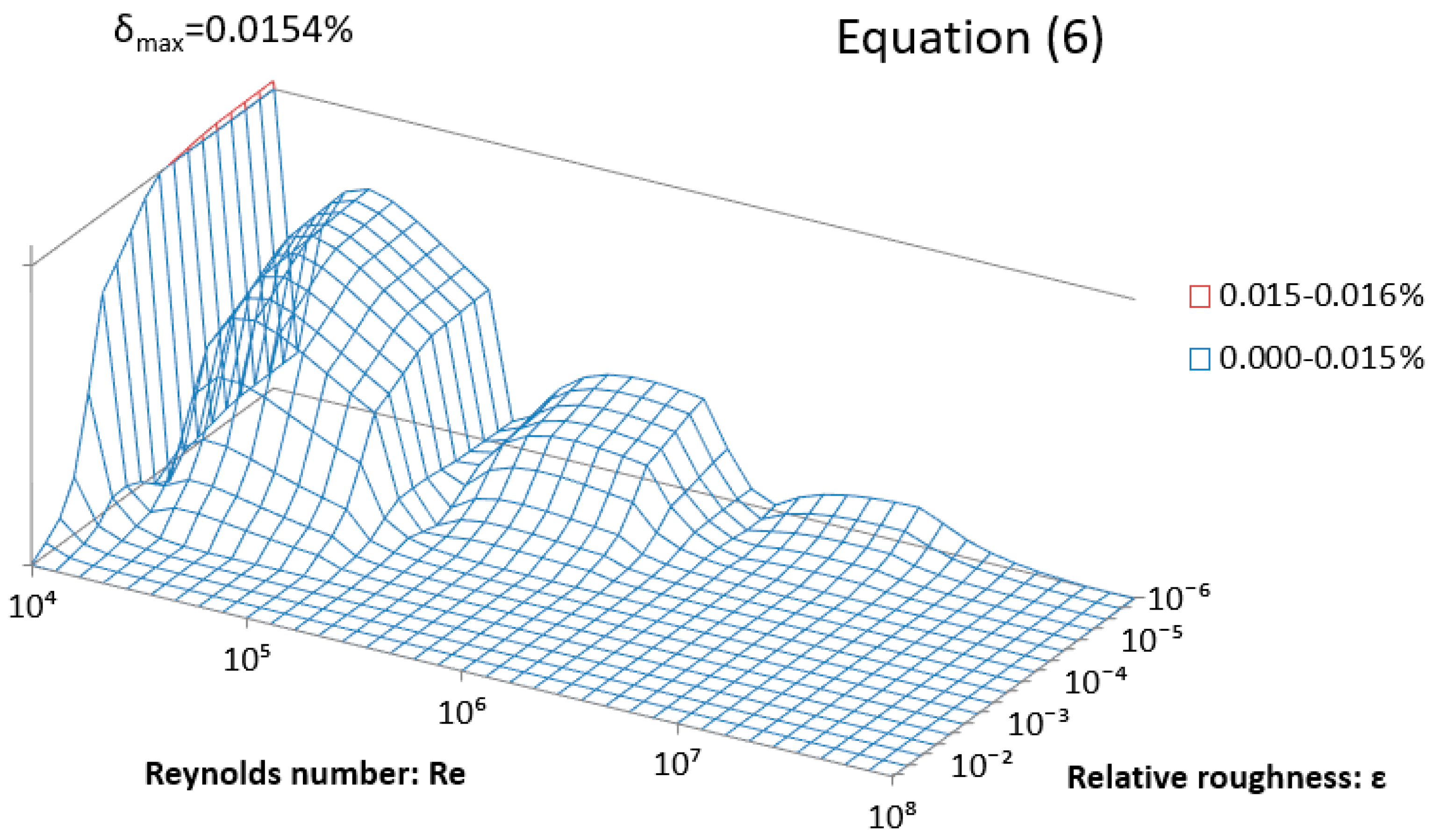
Max. Rel. Error %	740 Test Points 1	2 Million Test Point 2
Equation (3)	0.79%	1.81%
Equation (4)	0.101%	0.156%
Equation (5)	0.172%	0.317%
Equation (6)	0.0154%	0.0259%

¹ Reynolds number Re from 10⁴ to 10⁸. ² Reynolds number Re from 4000 to 10⁸.

. The same value of the maximal error is detected for even 2000 quasi Monte-Carlo points. Thus, this analysis confirms that the Sobol sequence of 2 million quasi Monte-Carlo points sufficiently covers the whole domain. For example, for Equation (6), the largest relative error is detected for the input pair Re = 5263 and $\epsilon$ = 3.1707 × 10⁻⁷, which corresponds to the zone with lower Reynolds numbers. Although this input pair is not shown in Figure 2, Figure 3, Figure 4 and Figure 5, the figures clearly indicate a tendency towards higher relative errors when the Reynolds number $Re$ and the relative roughness of the inner pipe surface $\epsilon$ are smaller.

As shown in Figure 6, additional analysis in MS Excel for the zone 4000 < $\mathit{Re}$ < 10⁴ shows very good agreement with the results obtained in Matlab.

4. Description of Software

The presented approximations were thoroughly tested at IT4Innovations, National Supercomputing Center, VŠB (Technical University of Ostrava, Czech Republic). For simplicity, the codes were expressed in MS Excel format [42] and in Matlab. The Matlab codes also work in GNU Octave, but they can be easily translated in any programming language.

Software codes in MS Excel are given in Supplementary Materials. However, we provide Matlab codes here, in order to support the benchmark study of the Colebrook equation [35] (in addition these Matlab codes are also given in Supplementary Materials).

Equation (3): An explicit approximation with one internal iterative cycle and with a fixed starting point.

Matlab code:

x = 16.9/2.51;
y0 = 2.51*x./R + K./3.71;
x1 = −2*log10(y0);
z = y0./((K/3.71) + (2.51*x1./R));
ln11 = @(z) (z.*(z + 4) − 5)./(4*z + 2);
x = x1 + 0.8686*ln11(z);
f = 1./x.^2;

In the Matlab codes, the Reynolds number Re is noted as R, while the relative roughness of the inner pipe surface ε is K.

Equation (4): An explicit approximation with one internal iterative cycle and a rational starting point given by Equation (2).

Matlab code:

For the rational starting point, x is given by Equation (2), as follows:

x = (2600*R)./(657.7*R + 214600*R.*K + 12970000) − 13.58*K + (0.0001165*R)./(0.00002536*R + R.*K + 105.5) + 4.227;

The rest of the Matlab code is unchanged.

Equation (5): An explicit approximation with two internal iterative cycles and a fixed starting point.

Matlab code:

x = 16.9/2.51;
y0 = 2.51*x./R + K./3.71;
x1 = −2*log10(y0);
z = y0./((K/3.71) + (2.51*x1./R));
ln11 = @(z) (z.*(z + 4) − 5)./(4*z + 2);
x = x1 + 0.8686*ln11(z);
z = y0./((K/3.71) + (2.51*x./R));
x = x1 + 0.8686*ln11(z);
f = 1./x.^2;

Equation (6): An explicit approximation with two internal iterative cycles and a rational starting point given by Equation (2).

Matlab code:

For the rational starting point, x is given by Equation (2). The rest of the Matlab code is unchanged.

5. Conclusions

This article presents simplified, but still precise algorithms for solving the Colebrook equation based on a fixed-point iterative procedure in which the logarithm is replaced by its Padé approximant in all iterations except the first one [24]. Moreover, a novel simple starting point, which was found by symbolic regression, significantly reduces the error of internal iterations. Consequently, a cheap Padé approximant of the first order is suitable for approximations. Depending on the stopping criteria and number of iterations, this algorithm can solve the Colebrook equation with any desired accuracy. As the computationally expensive logarithmic function is used only in the first step, this algorithm can be used efficiently for simulations of a complex pipe network. This is because the carefully selected Padé approximants can save computational time. For a good balance between efficiency and accuracy [9], two explicit approximations have been demonstrated based on a simplified iterative procedure with a maximal relative error of no more than 1.81% and 0.156% for the variant with one internal iterative cycle, and of no more than 0.317% and 0.0259% for two internal cycles (higher error values are for the fixed initial starting point, while lower error values are for the initial starting point given by the rational function, Equation (2), respectively). The value of the relative error, and also the tendency of its distribution, are confirmed by 2 million quasi Monte-Carlo points using the Sobol sequence for 4000 < Re < 10⁸ and for 0 < ε < 0.05.

The presented approximations have an acceptable level of accuracy [43], especially in light of the fact that the Colebrook equation is empirical and by its nature not always accurate. We can see that iterations with the cheap Padé approximant of the first order have a nearly identical relative error to iterations with the logarithm. Consequently, the herein presented approximations are favorable, as they do not contain computationally demanding evaluations such as special functions, exponential functions, or non-integer powers.

References

- Colebrook, C.F. Turbulent flow in pipes with particular reference to the transition region between the smooth and rough pipe laws. J. Inst. Civ. Eng. 1939, 11, 133–156. [Google Scholar] [CrossRef]
- Corless, R.M.; Gonnet, G.H.; Hare, D.E.; Jeffrey, D.J.; Knuth, D.E. On the LambertW function. Adv. Comput. Math. 1996, 5, 329–359. [Google Scholar] [CrossRef]
- Hayes, B. Why W? On the Lambert W function, a candidate for a new elementary function in mathematics. Am. Sci. 2005, 93, 104–108. [Google Scholar] [CrossRef]
- Keady, G. Colebrook-White formula for pipe flows. J. Hydraul. Eng. 1998, 124, 96–97. [Google Scholar] [CrossRef]
- Sonnad, J.R.; Goudar, C.T. Constraints for using Lambert W function-based explicit Colebrook–White equation. J. Hydraul. Eng. 2004, 130, 929–931. [Google Scholar] [CrossRef]
- More, A.A. Analytical solutions for the Colebrook and White equation and for pressure drop in ideal gas flow in pipes. Chem. Eng. Sci. 2006, 61, 5515–5519. [Google Scholar] [CrossRef]
- Clamond, D. Efficient resolution of the Colebrook equation. Ind. Eng. Chem. Res. 2009, 48, 3665–3671. [Google Scholar] [CrossRef]
- Biberg, D. Fast and accurate approximations for the Colebrook equation. J. Fluids Eng. 2017, 139, 031401. [Google Scholar] [CrossRef]
- Brkić, D.; Praks, P. Accurate and efficient explicit approximations of the Colebrook flow friction equation based on the Wright ω-function. Mathematics 2019, 7, 34. [Google Scholar] [CrossRef]
- Praks, P.; Brkić, D. Choosing the optimal multi-point iterative method for the Colebrook flow friction equation. Processes 2018, 6, 130. [Google Scholar] [CrossRef]
- Zigrang, D.J.; Sylvester, N.D. Explicit approximations to the solution of Colebrook’s friction factor equation. AIChE J. 1982, 28, 514–515. [Google Scholar] [CrossRef]
- Winning, H.K.; Coole, T. Explicit friction factor accuracy and computational efficiency for turbulent flow in pipes. Flow Turbul. Combust. 2013, 90, 1–27. [Google Scholar] [CrossRef]
- Winning, H.K.; Coole, T. Improved method of determining friction factor in pipes. Int. J. Numer. Methods Heat Fluid Flow 2015, 25, 941–949. [Google Scholar] [CrossRef]
- Vatankhah, A.R. Approximate analytical solutions for the Colebrook equation. J. Hydraul. Eng. 2018, 144, 06018007. [Google Scholar] [CrossRef]
- Pimenta, B.D.; Robaina, A.D.; Peiter, M.X.; Mezzomo, W.; Kirchner, J.H.; Ben, L.H. Performance of explicit approximations of the coefficient of head loss for pressurized conduits. Rev. Bras. Eng. Agrícola Ambient. 2018, 22, 301–307. [Google Scholar] [CrossRef]
- Colebrook, C.; White, C. Experiments with fluid friction in roughened pipes. Proc. R. Soc. Lond. Ser. A Math. Phys. Sci. 1937, 161, 367–381. [Google Scholar] [CrossRef]
- Díaz-Damacillo, L.; Plascencia, G. A new six parameter model to estimate the friction factor. AIChE J. 2019, 65, 1144–1148. [Google Scholar] [CrossRef]
- McKeon, B.J.; Zagarola, M.V.; Smits, A.J. A new friction factor relationship for fully developed pipe flow. J. Fluid Mech. 2005, 538, 429–443. [Google Scholar] [CrossRef]
- Ekhtiari, A.; Dassios, I.; Liu, M.; Syron, E. A novel approach to model a gas network. Appl. Sci. 2019, 9, 1047. [Google Scholar] [CrossRef]
- Barreras, F.; López, A.M.; Lozano, A.; Barranco, J.E. Experimental study of the pressure drop in the cathode side of air-forced open-cathode proton exchange membrane fuel cells. Int. J. Hydrogen Energy 2011, 36, 7612–7620. [Google Scholar] [CrossRef]
- Stubbs, A.; Stoesser, T.; Bockelmann-Evans, B. Developing an approximation of a natural, rough gravel riverbed both physically and numerically. Geosciences 2018, 8, 449. [Google Scholar] [CrossRef]
- Möws, R.; Koll, K. Roughness Effect of submerged groyne fields with varying length, groyne distance, and groyne types. Water 2019, 11, 1253. [Google Scholar] [CrossRef]
- Mouza, A.A.; Skordia, O.D.; Tzouganatos, I.D.; Paras, S.V. A simplified model for predicting friction factors of laminar blood flow in small-caliber vessels. Fluids 2018, 3, 75. [Google Scholar] [CrossRef]
- Praks, P.; Brkić, D. One-log call iterative solution of the Colebrook equation for flow friction based on Padé polynomials. Energies 2018, 11, 1825. [Google Scholar] [CrossRef]
- Baker, G.A.; Graves-Morris, P. Padé Approximants, 2nd ed.; Cambridge University Press: Cambridge, UK, 1996. [Google Scholar]
- Copley, L. Padé Approximants. In Mathematics for the Physical Sciences; De Gruyter: Berlin, Germany, 2014; Chapter 7; pp. 163–179. [Google Scholar] [CrossRef]
- Kalateh Bojdi, Z.; Ahmadi-Asl, S.; Aminataei, A. A new extended Padé approximation and its application. Adv. Numer. Anal. 2013, 2013, 263467. [Google Scholar] [CrossRef]
- Peker, H.A.; Karaoğlu, O.; Oturanç, G. The differential transformation method and Padé approximant for a form of Blasius equation. Math. Comput. Appl. 2011, 16, 507–513. [Google Scholar] [CrossRef]
- Li, S.; Liu, X.; Zhang, X. A few iterative methods by using [1,n]-order Padé approximation of function and the improvements. Mathematics 2019, 7, 55. [Google Scholar] [CrossRef]
- Alfaro-Guerra, M.; Guerra-Rojas, R.; Olivares-Gallardo, A. Evaluación experimental de la solución analítica exacta de la ecuación de Colebrook-White (Experimental evaluation of exact analytical solution of the Colebrook-White Equation). Ingeniería Investigación y Tecnología 2019, 20, 1–11. (In Spanish) [Google Scholar] [CrossRef]
- Dubčáková, R. Eureqa: Software review. Genet. Program. Evol. Mach. 2011, 12, 173–178. [Google Scholar] [CrossRef]
- Schmidt, M.; Lipson, H. Distilling free-form natural laws from experimental data. Science 2009, 324, 81–85. [Google Scholar] [CrossRef]
- Gholamy, A.; Kreinovich, V. How to use absolute-error-minimizing software to minimize relative error: Practitioner’s guide. Int. Math. Forum 2017, 12, 763–770. [Google Scholar] [CrossRef][Green Version]
- Praks, P.; Brkić, D. Symbolic regression-based genetic approximations of the Colebrook equation for flow friction. Water 2018, 10, 1175. [Google Scholar] [CrossRef]
- Gorkemli, B.; Karaboga, D. A quick semantic artificial bee colony programming (qsABCP) for symbolic regression. Inf. Sci. 2019, 502, 346–362. [Google Scholar] [CrossRef]
- Brkić, D.; Ćojbašić, Ž. Intelligent flow friction estimation. Comput. Intell. Neurosci. 2016, 2016, 5242596. [Google Scholar] [CrossRef] [PubMed]
- Brkić, D.; Ćojbašić, Ž. Evolutionary optimization of Colebrook’s turbulent flow friction approximations. Fluids 2017, 2, 15. [Google Scholar] [CrossRef]
- Praks, P.; Brkić, D. Advanced iterative procedures for solving the implicit Colebrook equation for fluid flow friction. Adv. Civ. Eng. 2018, 2018, 5451034. [Google Scholar] [CrossRef]
- Brkić, D. Review of explicit approximations to the Colebrook relation for flow friction. J. Pet. Sci. Eng. 2011, 77, 34–48. [Google Scholar] [CrossRef]
- Sobol’, I.M.; Turchaninov, V.I.; Levitan, Y.L.; Shukhman, B.V. Quasi-Random Sequence Generators; Distributed by OECD/NEA Data Bank; Keldysh Institute of Applied Mathematics; Russian Academy of Sciences: Moscow, Russia, 1992; Available online: https://europa.eu/ (accessed on 28 August 2019).
- Bratley, P.; Fox, B.L. Algorithm 659: Implementing Sobol’s quasirandom sequence generator. ACM Trans. Math. Softw. 1988, 14, 88–100. [Google Scholar] [CrossRef]
- Brkić, D. Solution of the implicit Colebrook equation for flow friction using Excel. Spreadsheets Educ. 2017, 10, 4663. Available online: https://sie.scholasticahq.com/article/4663.pdf (accessed on 19 August 2019).
- Pérez-Pupo, J.R.; Navarro-Ojeda, M.N.; Pérez-Guerrero, J.N.; Batista-Zaldívar, M.A. On the explicit expressions for the determination of the friction factor in turbulent regime. Rev. Mex. Ing. Chim. 2020, 19, 313–334. [Google Scholar] [CrossRef]