Numerical Simulation Using Finite-Difference Schemes with Continuous Symmetries for Processes of Gas Flow in Porous Media

Abstract

This article presents the applications of continuous symmetry groups to the computational fluid dynamics simulation of gas flow in porous media. The family of equations for one-phase flow in porous media, such as equations of gas flow with the Klinkenberg effect, is considered. This consideration has been made in terms of difference scheme constructions with the preservation of continuous symmetries, which are presented in original parabolic differential equations. A new method of numerical solution generation using continuous symmetry groups has been developed for the equation of gas flow in porous media. Four classes of invariant difference schemes have been found by using known group classifications of parabolic differential equations with partial derivatives. Invariance of necessary conditions for stability has been shown for the difference schemes from the presented classes. Comparison with the classical approach for seeking numerical solutions for a particular case from the presented classes has shown that the calculation speed is greater by several orders than for the classical approach. Analysis of the accuracy for the presented method of numerical solution generation on the basis of continuous symmetries shows that the accuracy of generated numerical solutions depends on the accuracy of initial solutions for generations.

1. Introduction

Modern problems in modeling of natural oil and gas reservoirs require the use of complex coupled equations for physically different unsteady processes such as multiphase seepage, geomechanics, and multicomponent thermodynamical processes for three spatial dimensions. It would seem that simple models are not very useful nowadays. However, consideration of all processes straightly and completely at the same moment is extremely difficult, for example [1]. That is why one of the most popular topics in mathematical modeling of processes related to natural oil and gas reservoirs is how to simplify a model to a stage where it is still interesting and can be numerically solved with acceptable results [2]. All these approaches require reliable benchmark models, such as the mentioned simple equations, and a basis for their construction and numerical solving, for example, for a more effective choice of initial iterations. Moreover, methods with simple models can help in understanding how to use them in more complicated situations. Another application of simple models is for fast calculations in the field of petroleum engineering, where time is more important than model complexity in some cases.

Most real-life problems in modeling cannot be solved analytically and have to be replaced by some numerical algorithms from computational fluid dynamics. However, a particular numerical method should be reliable and fast enough to conduct many similar calculations when such algorithms are frequently used for different problems. Thus, they must be analyzed using different analytical methods, which can be originally created only for theoretical models. This analysis can help to speed up numerical calculations and increase their reliability.

A good example of the mentioned analytical methods is using Lie groups of transformations for difference schemes [3] as considered in this study. This theory was initially applied for differential equations [4] and proved to be a powerful instrument in analysis. It provides an opportunity to look at solving of equations systematically and classify similar equations in a sense of their symmetries. It means looking at different methods of solving differential equation from one point of view, namely, from theory of Lie symmetry groups. During the last century, Lie’s theory was improved, and many results for different types of partial differential equations appeared [5,6].

This approach is used for other types of equations; for example, there are a number of results about group analysis of difference equations [3,7], differential-difference equations [8], and discrete dynamical systems [9], but there are no precise answers in a sense of numerical benefits from using invariant different schemes. Moreover, this question is almost avoided because of its complexity. Thus, the main purpose of this study is to find and underline useful properties of the Lie point symmetry preservation for difference schemes in terms of computational fluid dynamics simulation.

2. Continuous Symmetries of Parabolic Equations of Flow in Porous Media

2.1. Lie Point Symmetries

Local Lie groups of transformations in a multidimensional Euclidian space are used in this article. These families of transformations depend on some continuous parameter and all together form a group in the meaning of abstract algebra. However, they fulfill group properties only locally, which means that some small open neighborhood of a continuous parameter exists for every value of a parameter where a family of transformations is a group.

Let us consider an r-parameter Lie group of transformations [5], i.e., a family of transformations with local group properties that depends on r essential parameters $a=(a_1,a_2,\dots ,a_r)\in {ℝ}^r$ and is defined as $x^{\prime }=f(x,a)$, where $x^{\prime },x\in D\subseteq {ℝ}^r$. For group analysis using this type of groups, another very important concept is an infinitesimal operator [6], which is defined as a differential operator

$$X={{\displaystyle \sum _{i=1}^n\frac{\partial f^i(x,a)}{\partial a}}|}_{a=0}\frac{\partial }{\partial x^i}={\displaystyle \sum _{i=1}^n{\xi }^i}(x)\frac{\partial }{\partial x^i},$$

where $x^{\prime }=f(x,a)$ is a one-parameter Lie group. This operator is the tangent space $\xi (x)=({\xi }^1(x),{\xi }^2(x),\dots ,{\xi }^n(x))$ of a continuous group of transformations.

Invariants of defined groups of transformations play an important role in group analysis of equations. They are functions $F(x),x\in {ℝ}^n$, which remain the same under the action of their transformation groups. A concept of an infinitesimal operator gives an opportunity to use the infinitesimal criterion [6] of invariance, which can be written as (1):

$$XF(x)={\displaystyle \sum _{i=1}^n{\xi }^i}\frac{\partial F}{\partial x^i}=0.$$

(1)

An invariant manifold for a Lie group of transformations is a manifold whose points are transformed into points of this manifold under the action of this symmetry group. The infinitesimal criterion for manifolds is almost the same apart from the necessity to cancel variables, which can be expressed explicitly via the definition of a manifold.

The approach of Lie groups of continuous symmetries allows to work with different types of equations as manifolds in a correspondent space. Thus, continuous or finite-difference derivatives are considered as other independent variables. The concept of Lie groups’ action prolongation helps to define new additional variables (for a transformation group), which are presented in an equation apart from the variables of a group. These new variables are considered with initial variables in the same way. One says that this group is a continuous symmetry group for this equation or this equation admits this continuous group if an equation is an invariant for the prolonged continuous group. In this concept within this article, different additional variables can be derivatives for differential equations or finite-difference derivatives for difference equations.

The presence of a continuous symmetry for an equation defines a structure of connections between its solutions. Solutions can be transformed into each other by applying the group of transformations. This property gives an opportunity to generate families of solutions via one non-invariant solution and one symmetry group. It is demonstrated below for numerical solutions of constructed invariant different schemes.

This section is intended to provide basic ideas of theory of Lie groups for differential and difference equations. One can find more information about group analysis of differential equations in [5,6]. The results referring to the discrete case can be found in [3].

2.2. Group Classification Results for Parabolic Type Equations

One type of partial differential equations is considered in this article—the equations of gas flow in one-dimensional porous media [10]. The equations are as follows:

$$\frac{d\left(\rho (P)\phi (P)\right)}{dP}\frac{\partial P}{\partial t}-\frac{\partial }{\partial x}\left(\frac{K(P)\rho (P)}{\mu (P)}\frac{\partial P}{\partial x}\right)=0.$$

(2)

These equations represent an example of simple models for problems of gas flow in porous media, which are mentioned in the introduction. They can be written in the following form:

$$\frac{d\alpha }{dP}\frac{\partial P}{\partial t}-\frac{\partial }{\partial x}\left(\beta (P)\frac{\partial P}{\partial x}\right)=0,$$

(3)

what gives clear understanding that they are similar to the corresponding heat transfer equations. Different types of heat transfer equations are well researched in terms of group analysis by using Lie groups of point transformations [11]. Coefficients $\alpha$ and $\beta$ are used further for group classifications of these differential equations and their corresponding finite-difference representations. The group analysis is performed for this family of Equations (3) and can be found in [12] for the differential case. The group analysis results are partly presented in the section below for constructing of difference schemes with the preservation of continuous symmetries.

2.3. Gas Flow Equation with Klinkenberg Effect

Let us consider a particular example of Equations (2) with the equation of state for ideal gas with constant temperature $\rho =\chi P$ and with the Klinkenberg relationship for permeability [10,13], which is given by (4) as follows:

$$K(P)=K_1(1+K_2/P),$$

(4)

where $\phi =const$ and $\mu =const$. The equation for these coefficients can be written as

$$\frac{\partial P}{\partial t}-\gamma \frac{\partial }{\partial x}\left((P+K_2)\frac{\partial P}{\partial x}\right)=0,\gamma =\frac{K_1}{\mu \phi }.$$

(5)

This equation has four one-parameter groups of continuous symmetries with the infinitesimal operators [11,12]:

$$X_1=\frac{\partial }{\partial t},X_2=\frac{\partial }{\partial x},X_3=2t\frac{\partial }{\partial t}+x\frac{\partial }{\partial x},X_4=-t\frac{\partial }{\partial t}+(P+K_2)\frac{\partial }{\partial P}.$$

(6)

Continuous symmetries for differential equations may contain crucial properties of equations because these symmetries define connections between solutions. It is a very important property of symmetry groups as mentioned above, namely, the approach for solution generations using these transformation groups. For considered particular Equation (5), symmetries with $X_1$ and $X_2$ stand for translations of time and spatial variable, respectively. Thus, Equation (5) does not explicitly present time and spatial variables. The operator $X_3$ is responsible for the dilation symmetry of (5) or, to be more precise, for the parabolic differential structure of the equation. The symmetry with the operator $X_4$ is due to the particular form of the coefficient $\beta$ from (3).

3. Construction of Invariant Difference Schemes

3.1. Difference Scheme Construction with Preservation of Symmetries

Difference scheme construction with the preservation of continuous symmetries for an original differential equation has been previously presented in [3]. This method is used in this study to obtain all possible invariant difference schemes without restrictions to certain forms of finite-difference derivatives or neighboring points for the current point of a mesh.

Let us consider some differential equation

$$F_i(x,y,\underset{1}{y},\underset{2}{y},\dots ,\underset{p}{y})=0,i=1\dots q,x\in {ℝ}^n,y\in {ℝ}^m,$$

(7)

where $\underset{j}{y}$ is a set of $j$ order derivatives for the function $y(x)$ and $p$ is the order of (7). Let Equation (7) has an $r$-parameter symmetry group of transformations, which is a Lie group

$$\begin{array}{l}{\overline{x}}^i=f^i(x,y,a),{\overline{y}}^j=g^j(x,y,a),\\ a\in {ℝ}^r,\overline{x}\in {ℝ}^n,\overline{y}\in {ℝ}^m,i=1\dots n,j=1\dots m\end{array}$$

(8)

with $r$ infinitesimal operators

$$X_j={\displaystyle \sum _{i=1}^n{\xi }_j^i(x,y)\frac{\partial }{\partial x^i}}+{\displaystyle \sum _{i=1}^m{\eta }_j^i(x,y)}\frac{\partial }{\partial y^i}.$$

(9)

Equation (7) can be written via differential invariants $I_j$ [5,6] of the symmetry group (8), which can be found from Equation (1) and written as

$${\mathsf{\Phi }}_i(I_1,I_2,\dots ,I_s)=0,i=1\dots q,I_j=I_j(x,y,\underset{1}{y},\underset{2}{y},\dots ,\underset{p}{y}),j=1\dots s.$$

(10)

This set of functions $I_j$ is not unique because any smooth enough function of invariants is an invariant. Let us consider some difference scheme in the following form [14]:

$$\begin{array}{l}{E}_i(x_{k_0},y_{k_0},x_{k_1},y_{k_1},\dots ,x_{k_l},y_{k_l})=0,i=1\dots \overline{q},k_0,k_1,\dots ,k_l\in K\subset {\mathbb{Z}}^n,\\ M_j(x_{k_0},y_{k_0},x_{k_1},y_{k_1},\dots ,x_{k_l},y_{k_l})=0,j=1\dots \overline{n},x\in {ℝ}^n,y\in {ℝ}^m,\end{array}$$

(11)

where $E_i$ stands for a difference equation; $M_j$ stands for a mesh; $l$ is the order of the difference scheme (11); $k_0,k_1,\dots ,k_l\in K$ are n-tuples, which are responsible for positions on a mesh $M$ from an n-dimensional space. One says that this group of transformations is a symmetry group for Equation (11) if this equation defines an invariant manifold for the group of transformations (8), which is rewritten for all indices $k$ from (11) as follows:

$${\overline{x}}_k^i=f^i(x_k,y_k,a),{\overline{y}}_k^j=g^j(x_k,y_k,a),i=1\dots n,j=1\dots m,k\in K.$$

(12)

One says that (11) is an invariant difference scheme for differential Equation (7), or in (11), all symmetries of (7) are preserved if the difference scheme (11) in the limit tends to (7). Tending to the limit in this definition means that quantity $h_{\max }\to 0$ where

$$h_{\max }=\underset{\left|k_i-k_j\right|\le n,k_i,k_j\in K}{\max }\left|x_{k_i}-x_{k_j}\right|,$$

which means that neighboring points of a mesh tend to be closer. Difference invariants for the continuous group (12) should be determined to find an invariant difference scheme. Difference invariants can be found from the following system of equations:

$$\begin{array}{l}\underset{K}{X_j}Q(x_{k_0},y_{k_0},x_{k_1},y_{k_1},\dots ,x_{k_l},y_{k_l})=0,j=1\dots r,\\ \underset{K}{X_j}={\displaystyle \sum _{k\in K}^{}\left({\displaystyle \sum _{i=1}^n{\xi }_j^i(x_k,y_k)\frac{\partial }{\partial x_k^i}}+{\displaystyle \sum _{i=1}^m{\eta }_j^i(x_k,y_k)}\frac{\partial }{\partial y_k^i}\right)},\end{array}$$

(13)

where $\underset{K}{X_j}$ are prolongations of operators X_j for variables $x_{k_0},y_{k_0},x_{k_1},y_{k_1},\dots ,x_{k_l},y_{k_l},$ which are values for independent and dependent variables in points of a mesh with the set of indices $K$ for every point. Let functions $J_j(x_{k_0},y_{k_0},x_{k_1},y_{k_1},\dots ,x_{k_l},y_{k_l})=const,j=1\dots \overline{s}$ be the difference invariants, which are found from the system of Equations (13). The approximation of differential invariants (10) via difference invariance (13) is the next step for constructing invariant difference schemes, which can be written as

$$I_j(x,y,\underset{1}{y},\underset{2}{y},\dots ,\underset{p}{y})={\mathsf{\Phi }}_j(J_1,J_2,\dots ,J_{\overline{s}})+O(h_{\max }^{n_j}),j=1\dots s,$$

(14)

where $h_{\max }\to 0$, $n_j$ is the order of approximation. Invariant difference schemes for a differential equation are constructed by the following steps:

• Identify continuous symmetries for a differential equation of the form (7);
• Express a differential equation in terms of differential invariants as it is shown in Equation (10);
• Construct difference invariants for a symmetry group of the form (12);
• Approximate differential invariants (10) via difference invariants from (13);
• Notate Equation (10) via approximations (14) of differential invariants;
• Seek functions $M_j$ for a definition of a mesh, i.e., obtain expressions for independent variables.

The aforementioned definition is not rigorous and is intended to outline the concept. However, in the further usage of this definition, every arbitrary function, such as $F_i$, $E_i$, and $M_i$, are sufficient to define corresponding types of equations or other objects, for example, a continuous group of transformations. Of course, there can be a situation for this definition with just an invariant system of equations of type (11) and without a limit of type (7), but this approach allows all possible invariant schemes, including one with or without a limit.

Invariant difference schemes have essentially the same continuous symmetries, which, as it is shown below for (5), may contain important information about an equation. The main question of this article what are numerical benefits of using this type of difference schemes and it arises from several studies (for example [3]), which have complete theory of group analysis of difference schemes using theory of Lie groups but almost without analysis of stability, approximation, convergence, and applications in practical problems for invariant difference schemes.

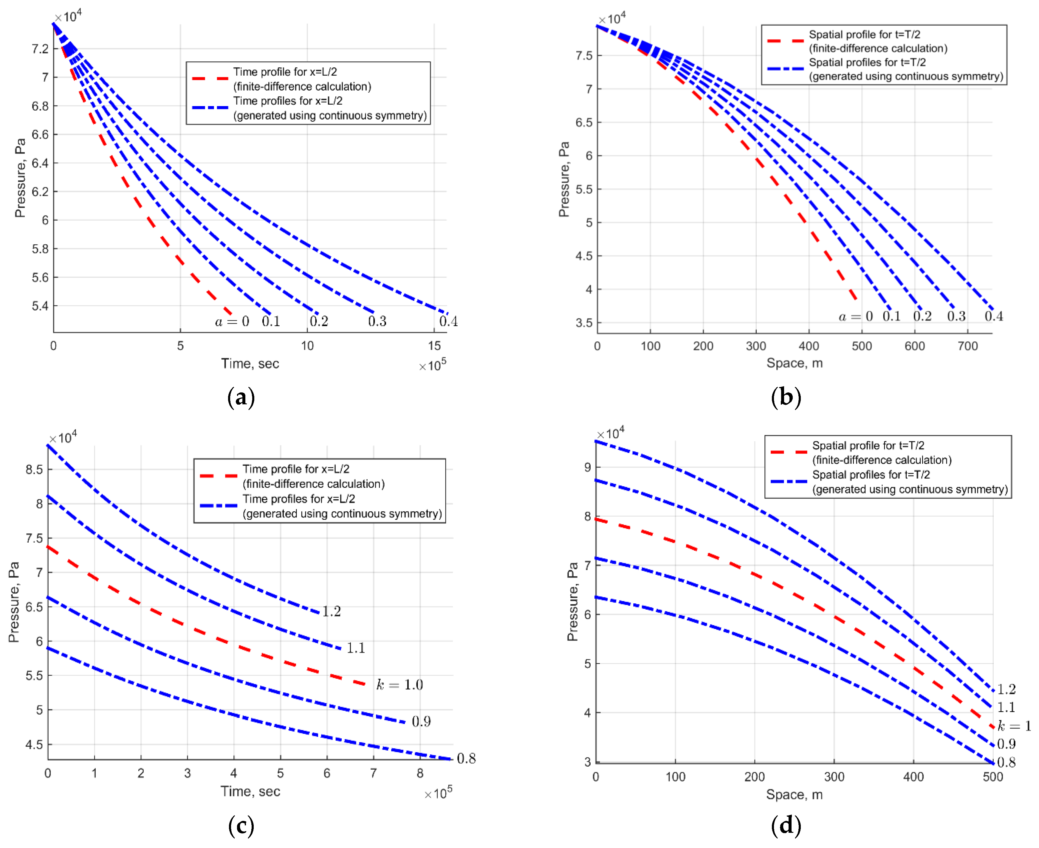
3.2. Numerical Solution Generation Using Continuous Symmetries

It is pointed out above that a particular solution can be transformed into another solution (providing that the first solution is not invariant) if a group of continuous symmetry is known. Therefore, one can obtain a family of solutions depending on a parameter of a group. This approach has been applied widely for differential equations and can be applied for difference schemes as well [3]. It provides an opportunity for calculating a numerical solution once and obtaining others by using a continuous group of symmetries but for some types of boundary and initial conditions, which must be transformed one into another by using the continuous group of symmetries. This problem is known and discussed in, for example, [15].

Let us consider a particular numerical solution, which is a set of points $\left\{(x_k,y_k)\right\}$, where k is an index on a mesh, $x_k$ is a vector of independent variables, and $y_k$ is a vector of dependent variables. It is an “ideal” numerical solution that is calculated using an “ideal” computer, which can avoid errors of truncations. Let us consider errors of truncations ${\epsilon }_k^1$ and ${\epsilon }_k^2$; thus, a “real” solution can be written as a set of points $\left\{(x_k+{\epsilon }_k^1,y_k+{\epsilon }_k^2)\right\}$. The errors are transformed when a transformation from some symmetry group is used for a correspondent difference scheme (which has the mentioned numerical solution) and new errors can be written as

$$\begin{array}{l}\overline{x}=f(x,a),\overline{y}=g(y,a),\\ {\overline{\epsilon }}_k^1=f(x_k+{\epsilon }_k^1,a)-f(x_k,a)+{\epsilon }_k^3(x_k,{\epsilon }_k^1,a),\\ {\overline{\epsilon }}_k^2=g(y_k+{\epsilon }_k^2,a)-g(y_k,a)+{\epsilon }_k^4(y_k,{\epsilon }_k^2,a),\end{array}$$

where ${\overline{\epsilon }}_k^1$ and ${\overline{\epsilon }}_k^2$ are errors for a generated solution using a continuous group of symmetry, ${\epsilon }_k^3$ and ${\epsilon }_k^4$ are errors for calculations of functions $f$ and $g$ using a “real” computer. Errors ${\overline{\epsilon }}_k^1$ and ${\overline{\epsilon }}_k^2$ tend to zero if ${\epsilon }_k^1$, ${\epsilon }_k^2$, ${\epsilon }_k^3$, and ${\epsilon }_k^4$ tend to zero. It is assumed that functions $f$ and $g$ are continuous and some converging algorithm is used to calculate them. Therefore, errors for solutions can be controlled and decreased when solutions are generated by symmetry groups. The nature of a used particular solution is not discussed in this section, so it can be, for example, unstable. However, it is not important in the case of this section.

3.3. Example of Invariant Difference Scheme Construction for Gas Flow Equation

Let us return to example (5) and conduct all the steps from the definition above. First of all, it is suggested to change the dependent variable $P$ using the following substitution:

$$\overline{P}={\displaystyle \underset{0}{\overset{P}{\int }}\gamma (x+K_2)}dx.$$

Thus, Equation (5) can be rewritten as

$$\frac{\partial P}{\partial t}-\sqrt{2\gamma P+{(\gamma K_2)}^2}\frac{{\partial }^{2}P}{\partial x^2}=0,$$

(15)

where the bar above for the new variable $\overline{P}$ is omitted in this section for the sake of convenience. This change of variables is made only for the following stability analysis. The symmetry group operators are the same (operators (6)) apart from the last for the new equation:

$$X_1,X_2,X_3,X_4=-t\frac{\partial }{\partial t}+(2P+\gamma K_2^2)\frac{\partial }{\partial P}.$$

(16)

For the symmetry group on the basis of (16), a differential invariant for an invariant notation of the form (10) can be chosen as follows:

$$I_1=\frac{P_{xx}\sqrt{2\gamma P+{(\gamma K_2)}^2}}{P_t}.$$

the continuous group from (16) has three other differential invariants, but they are omitted because the invariant notation for Equation (15) is $I_1=1$. Difference invariants for (16) can be written as follows

$$\begin{array}{l}{J}_1=\frac{{(x_{k+p_1}-x_{k+p_2})}^2}{(t^{n+p_3}-t^{n+p_4})\sqrt{2\gamma P_{k+p_5}^{n+p_6}+{(\gamma K_2)}^2}},J_2=\frac{2P_{k+p_7}^{n+p_8}+\gamma K_2^2}{2P_{k+p_9}^{n+p_{10}}+\gamma K_2^2},\\ J_3=\frac{x_{k+p_{11}}-x_{k+p_{12}}}{x_{k+p_{13}}-x_{k+p_{14}}},p_i\in \mathbb{Z}\end{array}$$

(17)

and can be obtained from the system of first-order partial differential equations of the form (13) with prolonged operators for (16). The numbers of invariants depend on the number (four in this case) of independent operators (in a sense of functional independence in the space of all discrete variables) and on the number of all discrete variables. The number of discrete variables can be chosen for this case as 17 for time (two time layers), spatial, and pressure variables in five nods of a mesh: central, top, bottom, left, and right nods. The number of invariants is greater than three, but there are only three different forms (17) of these invariants. The constants $p_i\in \mathbb{Z}$ are needed for expressing of all invariants and wider sets of invariant difference schemes, for example, for using different numbers of neighbor points for approximations of differential derivatives. These translations (constants $p_i$) are possible because of the specific form of operators (16), which can be shown as

$$X_j={\displaystyle \sum _{i=1}^n{\xi }_j^i(x^i)\frac{\partial }{\partial x^i}}+{\displaystyle \sum _{i=1}^m{\eta }_j^i(y^i)}\frac{\partial }{\partial y^i}.$$

The invariant $J_1$ allows to define the next time step according to the spatial variable steps and the current values of pressure $P_k^n$. The invariant $J_3$ defines possible spatial meshes including uniform meshes and $J_2$ comes from the operator $X_4$, which allows to scale pressure according to time.

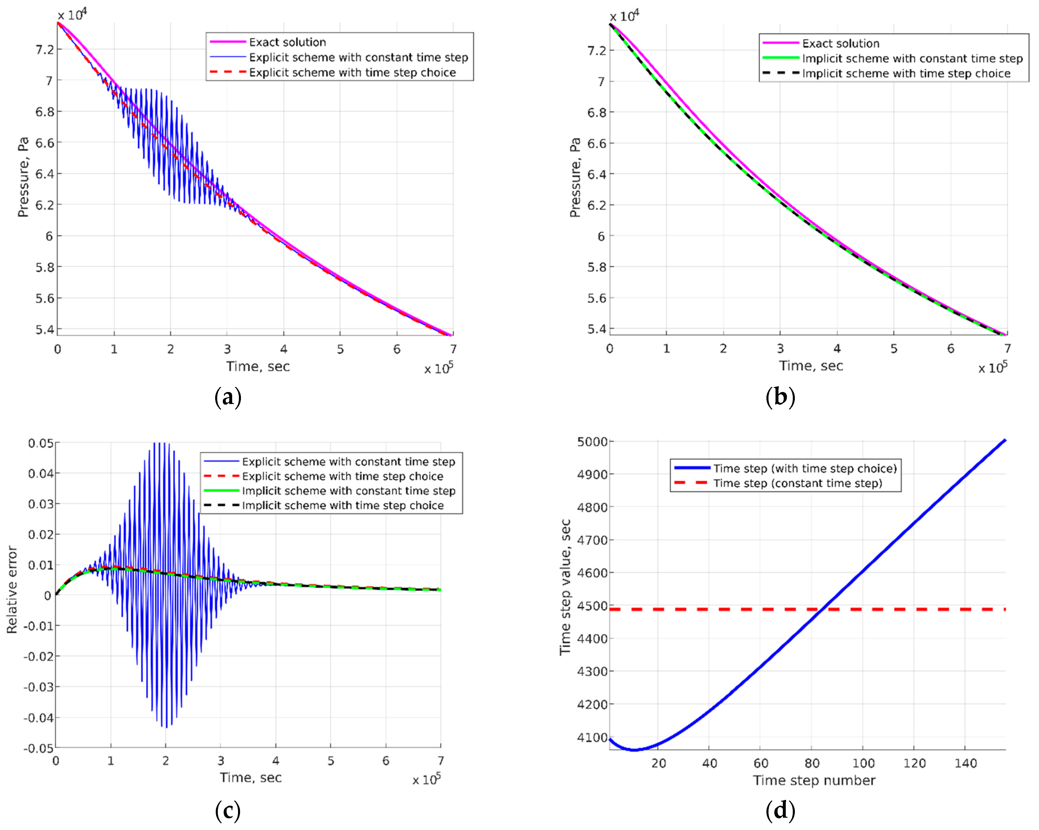
Let us consider two invariant difference schemes for deeper understanding of the difference invariant $J_1$: explicit

$$\frac{P_k^{n+1}-P_k^n}{t^{n+1}-t^n}-\frac{\sqrt{2\gamma P_k^n+{(\gamma K_2)}^2}(P_{k+1}^n-2P_k^n+P_{k-1}^n)}{(x_{k+1}-x_k)(x_k-x_{k-1})}=0$$

(18)

and implicit

$$\frac{P_k^{n+1}-P_k^n}{t^{n+1}-t^n}-\frac{\sqrt{2\gamma P_k^n+{(\gamma K_2)}^2}(P_{k+1}^{n+1}-2P_k^{n+1}+P_{k-1}^{n+1})}{(x_{k+1}-x_k)(x_k-x_{k-1})}=0$$

(19)

difference schemes. These difference schemes can be obtained via difference invariants (17). One can obtain necessary conditions for stability of the difference schemes (18) and (19) using the method of frozen coefficients [16]:

$$\frac{2(t^{n+1}-t^n)\underset{k}{\max }\sqrt{2\gamma P_k^n+{(\gamma K_2)}^2}}{(x_{k+1}-x_k)(x_k-x_{k-1})}<1,\frac{2(t^{n+1}-t^n)\underset{k}{\max }\sqrt{2\gamma P_k^n+{(\gamma K_2)}^2}}{(x_{k+1}-x_k)(x_k-x_{k-1})}>0.$$

(20)

The invariant $J_1$ can be rewritten as

$$J_1=\frac{{(x_{k+1}-x_k)}^2}{(t^{n+1}-t^n)\underset{k}{\max }\sqrt{2\gamma P_k^n+{(\gamma K_2)}^2}}=C=const.$$

It indicates that necessary conditions (20) for (18) and (19) are invariants but for different sets of values for the constant $C$. This fact gives an example of the continuous symmetry preservation importance for difference schemes. Of course, there are examples of difference schemes that can have more fruitful properties for numerical calculations and cannot be invariant. However, the described above approach allows us to have a very wide choice of difference schemes, which can be potentially better.

3.4. Families of Invariant Difference Schemes

The example from the last section shows very close connections between symmetries and properties of equations. It is applicable for both differential and difference cases. Differential equations of the type (3), which represents different problems for gas flow in porous media, are well researched by using theory of Lie groups. As it is mentioned above, this type of equations has group classifications, which can be found in [11,12]. These results and results from the last sections are used in the current section to obtain the families of invariant difference schemes for differential equations of the type (3), which stand for the physical problem (2). The aim of this section is to present only differential equations and their invariant difference schemes with coefficients, which can be chosen from real physical problems of gas flow in porous media. Thus, the results in

Table 1. Invariant difference schemes for gas flow equations.

No.	$\mathit{\alpha }$	$\mathit{\beta }$	Operators	Difference Invariants
1	$\alpha =c_{1}P+c_2$	$\beta =c_3{e}^P$	$X_1,X_2,X_3,$ ${\overline{X}}_4=x\frac{\partial }{\partial x}+2\frac{\partial }{\partial P}$	$J_1=\frac{(x_{k+p_1}-x_{k+p_2})(x_{k+p_3}-x_{k+p_4})}{(t^{n+p_5}-t^{n+p_6})e^{P_{k+p_{{}_8}}^{n+p_{{}_7}}}},$ $J_2=P_{k+p_{10}}^{n+p_9}-P_{k+p_{12}}^{n+p_{11}},$ $J_3=\frac{t^{n+p_{13}}-t^{n+p_{14}}}{t^{n+p_{15}}-t^{n+p_{16}}}$
2	$\alpha =c_{1}P+c_2$	$\beta =c_3{P}^{c_4},$ $c_4\ne 0,-\frac{4}{3}$	$X_1,X_2,X_3,$ ${\overline{X}}_4=\frac{c_4}{2}x\frac{\partial }{\partial x}+P\frac{\partial }{\partial P}$	$J_1=\frac{(x_{k+p_1}-x_{k+p_2})(x_{k+p_3}-x_{k+p_4})}{(t^{n+p_5}-t^{n+p_6}){(P_{k+p_8}^{n+p_7})}^{c_4}},$ $J_2=P_{k+p_{10}}^{n+p_9}/P_{k+p_{12}}^{n+p_{11}},$ $J_3=\frac{t^{n+p_{13}}-t^{n+p_{14}}}{t^{n+p_{15}}-t^{n+p_{16}}}$
3	$\alpha =c_{1}P+c_2$	$\beta =c_3{P}^{-4/3}$	$X_1,X_2,X_3,$ ${\overline{X}}_4=-\frac{2}{3}x\frac{\partial }{\partial x}+P\frac{\partial }{\partial P},$ ${\overline{X}}_5=-x^2\frac{\partial }{\partial x}+3xP\frac{\partial }{\partial P},$	$\begin{array}{c}{J}_1=\frac{P_{k+p_2}^{n+p_1}{(x_{k+p_2}-x_{k+p_3})}^{3/2}}{{(x_{k+p_3}-x_{k+p_4})}^{3/2}}\times \\ \times \frac{{(x_{k+p_2}-x_{k+p_4})}^{3/2}}{{(t^{n+p_5}-t^{n+p_6})}^{3/4}},\end{array}$ $J_2=\frac{t^{n+p_7}-t^{n+p_8}}{t^{n+p_9}-t^{n+p_{10}}},$ $J_3=\frac{(x_{k+p_{11}}-x_{k+p_{12}})(x_{k+p_{13}}-x_{k+p_{14}})}{(x_{k+p_{12}}-x_{k+p_{14}})(x_{k+p_{11}}-x_{k+p_{13}})}$
4	$\begin{array}{l}\frac{d\alpha }{dP}=c_3{e}^{-P}\times \\ \times {(c_1-e^{-P})}^{c_2}\end{array}$	$\beta =c_4{e}^{-P}$	$X_1,X_2,$ $\begin{array}{l}{\overline{X}}_3=c_{2}t\frac{\partial }{\partial t}+\\ +(c_1{e}^P-1)\frac{\partial }{\partial P},\end{array}$	$J_1=\frac{(t^{n+p_1}-t^{n+p_2})e^{c_2{P}_{k+p_4}^{n+p_3}}}{{(c_1{e}^{P_{k+p_4}^{n+p_3}}-1)}^{c_2}},$ $J_2=\frac{(c_1{e}^{P_{k+p_6}^{n+p_5}}-1)}{(c_1{e}^{P_{k+p_8}^{n+p_7}}-1)}{e}^{P_{k+p_8}^{n+p_7}-P_{k+p_6}^{n+p_5}},$ $J_3=x_{k+p_5}-x_{k+p_6}.$

are not intended to cover all equations from the known classifications.

In Table 1, $p_i\in \mathbb{Z}$ and $c_j\in ℝ$ are arbitral constants, and operators $X_1$, $X_2$, and $X_3$ are from (6). The results from Table 1 match results from [17] for cases 1–3 and certain constants $p_i$. The example (5) and all results for (15) belong to case 2 in Table 1 (with changing of variables $\overline{P}=P+K_2$) with coefficients $\frac{d\alpha }{dP}=P$ and $\beta =P$.

The one-dimensional case is considered for simplicity, and all results of this article can be generalized for the multidimensional case. All cases from Table 1 can have certain coefficients with certain physical meanings, and difference invariants can be used for constructing a wide set of invariant difference schemes. Another reason of class choices from known group classifications of differential equations of the parabolic type is the possibility of finding explicit forms for difference invariants and transformations from continuous symmetry groups, which can both be found from their corresponding equations.

Equation (2) and its classes from Table 1 can represent wide spectrums of problems for flow in porous media on different scales: microscale of pores, macroscale of fields, and other intermediate scales. For example, problems of CO₂ geological storage [18] or, in particular, problems of CO₂ injection on macroscales of porous media [19] can be studied using the results obtained from this study. There are several results for microscales that can be studied using results of this article for some specific cases of initial and boundary conditions, forms of pore network models and methods for calculating conductivities: suggested models for gas flow in [20], one-phase flow in [21], multiphase flow in [22], and modeling of films in gas–liquid–capillary systems in [23].

4. Numerical Results and Discussion

4.1. Choice of Time Step in Accordance with Difference Invariants

Example (5) is used for further results in this section. The explicit difference equation

$$\frac{P_k^{n+1}-P_k^n}{{\tau }^n}-\frac{\gamma }{h^2}\left((P_{k+1}^n-P_k^n)(P_k^n+K_2)-(P_k^n-P_{k-1}^n)(P_{k-1}^n+K_2)\right)=0,$$

(21)

the implicit difference equation

$$\frac{P_k^{n+1}-P_k^n}{{\tau }^n}-\frac{\gamma }{h^2}\left((P_{k+1}^{n+1}-P_k^{n+1})(P_k^n+K_2)-(P_k^{n+1}-P_{k-1}^{n+1})(P_{k-1}^n+K_2)\right)=0,$$

(22)

and the difference mesh

$$h=x_{k+1}-x_k=const,{\tau }^n=t^{n+1}-t^n=\frac{A{h}^2}{({\overline{P}}_{}^n+K_2)},$$

(23)

are used for numerical calculations, where $A$ is a coefficient that depends on the maximum time value and

Table 2. Parameters for numerical calculations.

Parameter	Value
$P_{left}$	100,000 Pa
$P_{right}$	10,000 Pa
$T$	700,000 s
$L$	500 m
$N_t$	157
$N_x$	10
$\phi$	0.20
$\mu$	10-6 Pa·s
$K_1$	10-12 m2
$K_2$	10 Pa
$C_2$	150,000 s

gives parameters for numerical calculations. The explicit difference scheme (21) and (23) were chosen for the sake of application demonstrations of the obtained invariant necessary conditions for stability. Figure 1 shows a comparison of numerical solutions for the difference scheme (21) and (23) and the difference scheme (22) and (23) (with the constant time step and with the time step choosing) and the exact solution, which is from [24]. The exact solution can be written as

$$P(t,x)=-\frac{{(x+C_1)}^2}{6\gamma (t+C_2)}+\frac{C_3}{{\left|t+C_2\right|}^{\frac{1}{3}}}-K_2,$$

where constants $C_1$ and $C_3$ depend on initial pressures (on the left and right boundaries) and constant $C_2$ is for the initial time value. Initial and boundary conditions for the difference scheme are chosen in accordance with the aforementioned solution. The comparison (Figure 1) of implicit difference schemes with (the time step choosing) and without (the constant time step) continuous symmetry groups from Table 1 shows almost no difference in numerical solutions. The comparison of explicit difference schemes shows that the time step choice (the case with continuous symmetries) from (23) helps to stabilize the explicit difference scheme (21) with the same number of constant time steps (the case without continuous symmetries).

Table A3. Comparisons of average absolute values of relative errors (in comparison with the exact solution) for used difference schemes and the generation method.

${\mathit{N}}_{\mathit{t}}$	${\mathit{N}}_{\mathit{x}}$
	5	10	15	20	25	30
91	0.006037	>1	>1	>1	>1	>1
	0.005821	>1	>1	>1	>1	>1
	0.005652	0.003276	0.002113	0.001473	0.001072	0.000797
	0.005424	0.003106	0.001989	0.001375	0.000989	0.000724
	0.005652	0.003276	0.002113	0.001473	0.001072	0.000797
157	0.006038	0.003699	>1	>1	>1	>1
	0.005842	0.006621	>1	>1	>1	>1
	0.005813	0.003498	0.002353	0.001722	0.001325	0.001054
	0.005611	0.003344	0.002242	0.001635	0.001253	0.000992
	0.005813	0.003498	0.002353	0.001722	0.001325	0.001054
393	0.006058	0.003767	0.002629	>1	>1	>1
	0.005859	0.003625	>1	>1	>1	>1
	0.005968	0.003686	0.002555	0.001934	0.001541	0.001272
	0.005766	0.003541	0.002453	0.001851	0.001473	0.001214
	0.005968	0.003686	0.002555	0.001934	0.001541	0.001272
778	0.006057	0.003787	0.002662	0.002039	>1	>1
	0.005864	0.003649	0.002561	>1	>1	>1
	0.006011	0.003745	0.002624	0.002003	0.001612	0.001343
	0.005817	0.003607	0.002522	0.001922	0.001546	0.001288
	0.006011	0.003745	0.002624	0.002003	0.001612	0.001343
1327	0.006058	0.003797	0.002675	0.002053	0.001662	>1
	0.005866	0.003659	0.002574	0.001975	0.01036	>1
	0.006031	0.003772	0.002652	0.002032	0.001642	0.001374
	0.005839	0.003634	0.002551	0.001953	0.001576	0.001319
	0.006031	0.003772	0.002652	0.002032	0.001642	0.001374
1830	0.00606	0.003799	0.002679	0.002058	0.001668	0.001498
	0.005867	0.003663	0.002579	0.00198	0.001604	>1
	0.006041	0.003782	0.002663	0.002043	0.001653	0.001386
	0.005847	0.003645	0.002563	0.001964	0.001588	0.001331
	0.006041	0.003782	0.002663	0.002043	0.001653	0.001386

and

Table A4. Comparisons of maximum absolute values of relative errors (in comparison with the exact solution) for used difference schemes and the generation method.

${\mathit{N}}_{\mathit{t}}$	${\mathit{N}}_{\mathit{x}}$
	5	10	15	20	25	30
91	0.028301	>1	>1	>1	>1	>1
	0.02818	>1	>1	>1	>1	>1
	0.027267	0.013512	0.008603	0.00599	0.004361	0.003294
	0.02706	0.013277	0.008376	0.005749	0.004129	0.003056
	0.027267	0.013512	0.008603	0.00599	0.004361	0.003294
157	0.028784	0.014194	>1	>1	>1	>1
	0.028729	0.062449	>1	>1	>1	>1
	0.028171	0.01446	0.009529	0.006937	0.005313	0.004233
	0.02806	0.014325	0.009397	0.006799	0.005176	0.004097
	0.028171	0.01446	0.009529	0.006937	0.005313	0.004233
393	0.029195	0.015153	0.009979	>1	>1	>1
	0.029169	0.015088	>1	>1	>1	>1
	0.028944	0.015264	0.010311	0.007739	0.006125	0.00503
	0.028895	0.01521	0.010258	0.007683	0.006068	0.004972
	0.028944	0.015264	0.010311	0.007739	0.006125	0.00503
778	0.029329	0.015475	0.010363	0.007758	>1	>1
	0.029316	0.015443	0.010322	>1	>1	>1
	0.029201	0.015531	0.010571	0.008006	0.006395	0.005301
	0.029177	0.015504	0.010544	0.007977	0.006366	0.005272
	0.029201	0.015531	0.010571	0.008006	0.006395	0.005301
1327	0.029385	0.015612	0.01054	0.007973	0.006361	>1
	0.029378	0.015593	0.01051	0.007941	0.57243	>1
	0.02931	0.015645	0.010682	0.008119	0.00651	0.005416
	0.029296	0.015629	0.010666	0.008102	0.006493	0.005399
	0.02931	0.015645	0.010682	0.008119	0.00651	0.005416
1830	0.029407	0.015666	0.010622	0.008057	0.006446	0.020468
	0.029402	0.015652	0.0106	0.008034	0.006423	>1
	0.029353	0.015689	0.010725	0.008163	0.006554	0.005461
	0.029343	0.015678	0.010714	0.008151	0.006542	0.005449
	0.029353	0.015689	0.010725	0.008163	0.006554	0.005461

show errors for different methods and meshes.

The comparison in Figure 1 shows the advantages for calculations with the time step choice from (23). This approach for time steps is well-known (see for example [16]), but it arises from analysis using continuous symmetries. According to the method used for constructing the invariant difference schemes, this condition for stability does not have to appear at first sight. The parameters from Table 2 are chosen to provide graphical examples for the obtained numerical results and their plots.

4.2. Generation of Numerical Solutions

This section is intended to present results of generations of numerical solutions for the difference scheme (22) and (23) of differential Equation (5) of gas flow in porous media. There are results of numerical solution generations [25] for the Rapoport–Leas equation [26], which is a generalization of the Buckley–Leverett problem. For symmetry groups with operators $X_1$ and $X_2$ from (6), transformations for solutions mean translations for time and spatial variables, respectively. It means only moving of the meshes without changes for the difference equations. It would be more interesting for the generation to consider operators $X_3$ and $X_4$ from (6). The groups of transformations are

$$\begin{array}{l}\overline{t}=e^{2a}t,\overline{x}=e^{a}x,\overline{P}=P,\\ \overline{t}=e^{-a}t,\overline{x}=x,\overline{P}=\left(P+K_2\right)e^a-K_2\end{array}$$

(24)

for $X_3$ and $X_4$, respectively. In Figure 2, actions of (24) for the numerical solution from Figure 1 (the implicit scheme (22) and (23) with the continuous symmetry groups (24)) are used to show the concept of the solution generation method.

The used initial and boundary conditions were chosen for the sake of testing. Classes of initial and boundary conditions are not restricted to those from exact solutions. For example, classes of initial and boundary conditions can be constructed on the basis of two smooth enough functions, which provide sensible numerical solutions for difference schemes with continuous symmetries. Classes of conditions are constructed by applying transformations from these continuous symmetry groups to these two functions.

The use of the generation algorithm via continuous symmetries is faster by several orders than the use of difference schemes as it has been obtained during numerical calculations of this section and in [25].

Table A1. Comparisons of demanded memory (bytes) for used difference schemes and the generation method.

${\mathit{N}}_{\mathit{t}}$	${\mathit{N}}_{\mathit{x}}$
	5	10	15	20	25	30
91	11,280	-	-	-	-	-
	11,240	-	-	-	-	-
	11,456	22,736	34,536	46,736	59,336	72,336
	11,416	22,696	34,496	46,696	59,296	72,296
	11,200	22,000	32,920	43,840	54,760	65,680
157	19,320	37,920	-	-	-	-
	19,280	37,880	-	-	-	-
	19,496	38,576	58,296	78,416	98,936	119,856
	19,456	38,536	58,256	78,376	98,896	119,816
	19,240	37,840	56,680	75,520	94,360	113,200
393	47,880	94,560	141,720	-	-	-
	47,840	94,520	-	-	-	-
	48,056	95,216	143,256	191,216	239,936	289,056
	48,016	95,176	143,216	191,176	239,896	289,016
	47,800	94,480	141,640	188,320	235,360	282,400
778	94,560	186,960	279,600	372,240	-	-
	94,520	186,920	279,560	-	-	-
	94,736	187,616	281,136	375,056	469,736	564,816
	94,696	187,576	281,096	375,016	469,696	564,776
	94,480	186,880	279,520	372,160	465,160	558,160
1327	161,160	318,720	476,880	635,280	793,440	-
	161,120	318,680	476,840	635,240	793,400	-
	161,336	319,376	478,416	638,096	797,936	958,656
	161,296	319,336	478,376	638,056	797,896	958,616
	161,080	318,640	476,800	635,200	793,360	952,000
1830	222,120	439,680	657,960	876,240	1,094,640	1,312,800
	222,080	439,640	657,920	876,200	1,094,600	-
	222,296	440,336	659,496	879,056	1,099,136	1,319,376
	222,256	440,296	659,456	879,016	1,099,096	1,319,336
	222,040	439,600	657,880	876,160	1,094,560	1,312,720

and

Table A2. Comparisons of the calculation time (seconds) for used difference schemes and the generation method.

${\mathit{N}}_{\mathit{t}}$	${\mathit{N}}_{\mathit{x}}$
	5	10	15	20	25	30
91	0.00005	-	-	-	-	-
	0.00004	-	-	-	-	-
	0.000453	0.000531	0.000723	0.000915	0.00096	0.001142
	0.000522	0.000493	0.00064	0.000889	0.000905	0.001037
	0.000007	0.00001	0.000008	0.00001	0.000009	0.000012
157	0.000074	0.000087	-	-	-	-
	0.000064	0.000074	-	-	-	-
	0.000695	0.000879	0.001104	0.001379	0.001637	0.001803
	0.000626	0.000801	0.001042	0.001235	0.001469	0.00169
	0.000007	0.000007	0.000011	0.000011	0.000012	0.000013
393	0.000169	0.000189	0.000217	-	-	-
	0.000154	0.000171	-	-	-	-
	0.001765	0.002007	0.002667	0.003127	0.003826	0.00441
	0.001499	0.001889	0.002482	0.00302	0.003691	0.004244
	0.000007	0.000012	0.000016	0.000019	0.000057	0.00004
778	0.000325	0.000606	0.000649	0.00047	-	-
	0.000301	0.000466	0.000519	-	-	-
	0.003149	0.006344	0.008676	0.006607	0.007358	0.009251
	0.002967	0.006046	0.008522	0.005953	0.007102	0.008982
	0.000012	0.00002	0.000056	0.000047	0.000058	0.00006
1327	0.000546	0.000627	0.000704	0.000777	0.000877	-
	0.000507	0.000577	0.000652	0.000699	0.000777	-
	0.005217	0.006465	0.008528	0.010208	0.01245	0.015874
	0.004937	0.006182	0.008253	0.009838	0.012067	0.01505
	0.000015	0.00004	0.00005	0.000079	0.00009	0.000095
1830	0.000754	0.000855	0.000988	0.001091	0.001233	0.001353
	0.000696	0.000786	0.000884	0.000979	0.001093	-
	0.007129	0.008863	0.011792	0.014185	0.017199	0.021577
	0.006866	0.00908	0.011447	0.013763	0.016761	0.020993
	0.000035	0.000058	0.000078	0.000095	0.0001	0.000127

present demanded memory and calculation time, respectively, for different methods and meshes. This advantage allows faster and more effective solutions of many problems, which demand a considerable number of multivariate calculations: uncertainty analysis, history matching and upscaling. Moreover, the proposed approach of numerical solution generation can be accelerated by parallelization of three steps of the method:

• The first step of obtaining initial numerical solutions can be paralleled by using some known parallel algorithms for solving arising systems of linear algebraic equations [27];
• The second step of group parameters seeking for transformations can be paralleled using some known parallel algorithms for solving arising systems of nonlinear (in the general case) algebraic equations [28] but there is no need for that in our case because group parameters can be analytically expressed via functions of initial and boundary conditions;
• The last step of numerical solution generation using continuous groups of symmetries can be paralleled because every mesh point and pressure value of a new generated solution are calculated independently.

The obtained results encourage further attempts to understand connections of stability and continuous symmetries for difference schemes in general cases, for example, two- and three-dimensional cases of multiphase flow equations in porous media. Moreover, the question of conservation laws [29,30] is close to continuous symmetries and not discussed in this article. It can help in a wider understanding of problems, which are considered in the article.

The following are the main disadvantages of the presented method:

• It is difficult to find continuous symmetry groups for all known and widely used differential equations and difference schemes;
• One must know explicit forms of transformations from symmetry groups;
• Initial and boundary conditions must be from an invariant family of conditions.

A future goal of this study is to partly reduce the effect of these factors.

5. Conclusions

It is very important to have an opportunity for fast and reliable calculations for the practical usage of numerical algorithms in many fields. The presence of continuous symmetries gives a method of solution generations using only these continuous groups. One must calculate one numerical solution for an invariant difference scheme, which must not be trivial or invariant. Thereafter, a family of numerical solutions can be obtained using a continuous group of transformations.

Constructing difference schemes with the preservation of continuous Lie point symmetries is considered using the examples of the equations of gas flow in porous media. The examples and results of numerical calculations show very close connections between symmetries and properties of difference schemes such as invariant necessary conditions and the opportunity for numerical solution generations. Calculated difference invariants and given classifications for the considered family of differential equations can be used for checking frequently used difference schemes and for constructing new schemes. The described method of numerical solution generation can be applied for increasing accuracy and speed of computational fluid dynamics simulation of gas flow in porous media.

References

1. Islam, M.R.; Hossain, M.E.; Mousavizadegan, S.H.; Mustafiz, S.; Abou-Kassem, J.H. Advanced Petroleum Reservoir Simulation: Towards Developing Reservoir Emulators, 2nd ed.; Wiley: Hoboken, NJ, USA, 2016; pp. 1–592. [Google Scholar]
2. Aziz, K. Ten golden rules for simulation engineers. JPT 1989, 41, 1157. [Google Scholar]
3. Dorodnitsyn, V. Applications of Lie Groups to Difference Equations, 1st ed.; Taylor and Francis Group: Boca Raton, FL, USA, 2011; pp. 1–265. [Google Scholar]
4. Lie, S. Vorlesungen Uber Differentialgleichungen Mit Bekannten Infinitesimalen Transformationen; Teubner: Leipzig, Germany, 1891; pp. 1–568. [Google Scholar]
5. Ibragimov, N.H. A Practical Course in Differential Equations and Mathematical Modelling: Classical and New Methods. Nonlinear Mathematical Models. Symmetry and Invariance Principles; Higher Education Press, World Scientific: Singapore, 2009; pp. 1–364. [Google Scholar]
6. Ovsyannikov, L.V. Lectures on the Theory of Group Properties of Differential Equations, 1st ed.; Higher Education Press Limited Company: Beijing, China, 2013; pp. 1–140. [Google Scholar]
7. Bihlo, A.; Valiquette, F. Symmetry-Preserving Numerical Schemes. Symmetries Integr. Differ. Equ. 2017. Available online: https://arxiv.org/pdf/1608.02557.pdf (accessed on 24 August 2019).
8. Shen, S.; Jin, Y. Group classification of differential-difference equations: Low-dimensional Lie algebras. Acta Math. Appl. Sin. Engl. Ser. 2017, 33, 345–362. [Google Scholar] [CrossRef]
9. Markov, P.V. Group classification of discrete dynamical systems. Rus. J. Nonlin. Dyn. 2013, 9, 641–649. [Google Scholar]
10. Paulini, P. A Two-Parametric Model for Gas Flow in Low-Permeable Porous Materials. Transp. Porous Med. 2019, 128, 303–318. [Google Scholar] [CrossRef]
11. Lagno, V.I.; Spichak, S.V.; Stogniy, V.I. Symmetry Analysis of Evolutional Type Equations, 1st ed.; Institute of Computer Research: Moscow, Russia, 2004; pp. 1–392. [Google Scholar]
12. Baikov, V.A.; Gazizov, R.K.; Ibragimov, N.H.; Kovalev, V.F. Water Redistribution in Irrigated Soil Profiles: Invariant Solutions of the Governing Equation. Nonlinear Dyn. 1997, 13, 395–409. [Google Scholar] [CrossRef]
13. Zhang, C.; Ranjith, P.G. Experimental Study of Matrix Permeability of Gas Shale: An Application to CO2-Based Shale Fracturing. Energies 2018, 11, 702. [Google Scholar] [CrossRef]
14. Levi, D.; Olver, P.; Thomova, Z.; Winternitz, P. Symmetries and Integrability of Difference Equations, 1st ed.; Cambridge University Press: Cambridge, UK, 2011; pp. 1–360. [Google Scholar]
15. Zhang, Z.-Y. Partial symmetry of initial value problems. J. Math. Anal. Appl. 2017, 450, 814–828. [Google Scholar] [CrossRef]
16. Ryaben’kii, V.S.; Tsynkov, S.V. A Theoretical Introduction to Numerical Analysis, 1st ed.; Chapman and Hall/CRC: Boca Raton, FL, USA, 2006; pp. 1–552. [Google Scholar]
17. Dorodnitsyn, V.; Kozlov, R. The whole set of symmetry preserving discrete versions of a heat transfer equation with a source. J. Nonlinear Math. Phys. 1997, 10, 16–50. [Google Scholar] [CrossRef]
18. Aliakbar, K.; Ali, V.; Mohammadreza, R.; Reza, A. Carbon Dioxide Geological Storage (CGS)—Current Status and Opportunities. In Greenhouse Gases, 1st ed.; Llamas, B., Pous, J., Eds.; IntechOpen: London, UK, 2016; pp. 155–177. [Google Scholar]
19. Saini, D. Engineering Aspects of Geologic CO2 Storage. Synergy between Enhanced Oil Recovery and Storage, 1st ed.; Springer: Berlin, Germany, 2017; pp. 1–73. [Google Scholar]
20. Zhang, P.; Hu, L.; Meegoda, J.N.; Gao, S. Micro/Nano-pore Network Analysis of Gas Flow in Shale Matrix. Sci. Rep. 2015, 5, 1–11. [Google Scholar] [CrossRef] [PubMed]
21. Baychev, T.G.; Jivkov, A.P.; Rabbani, A.; Raeini, A.Q.; Xiong, Q.; Lowe, T.; Withers, P.J. Reliability of Algorithms Interpreting Topological and Geometric Properties of Porous Media for Pore Network Modelling. Transp. Porous Med. 2019, 128, 271–301. [Google Scholar] [CrossRef] [Green Version]
22. Yin, X.; Aslannejad, H.; de Vries, E.T.; Raoof, A.; Hassanizadeh, S.M. Droplet Imbibition into Paper Coating Layer: Pore-Network Modeling Simulation. Transp. Porous Med. 2018, 125, 239–258. [Google Scholar] [CrossRef] [PubMed] [Green Version]
23. Yiotis, A.G.; Stubos, A.K.; Boudouvis, A.G.; Tsimpanogiannis, I.N.; Yortsos, Y.C. Pore-Network Modeling of Isothermal Drying in Porous Media. Transp. Porous Med. 2005, 58, 63–86. [Google Scholar] [CrossRef]
24. Polyanin, A.D.; Zaitsev, V.F. Handbook of Nonlinear Partial Differential Equations, 2nd ed.; Chapman & Hall/CRC: Boca Raton, FL, USA, 2012; pp. 1–1912. [Google Scholar]
25. Markov, P.V.; Rodionov, S.P. The method of accelerations of serial numerical calculations for multiphase flow equations in porous media using continuous groups of symmetries. Autom. Telemech. Commun. Oil Ind. 2015, 12, 23–30. [Google Scholar]
26. Bibikov, P. Group classification of Rapoport–Leas equations. Lobachevskii J. Math. 2017, 38, 116–124. [Google Scholar] [CrossRef]
27. Rauber, T.; Rünger, G. Parallel Programming for Multicore and Cluster Systems, 2nd ed.; Springer: Berlin, Germany, 2013; pp. 1–516. [Google Scholar]
28. Bistran, I.; Maruster, S.; Mafteiu-Scai, L.O. Parallel Variants of Broyden’s Method. Algorithms 2015, 8, 774–785. [Google Scholar] [CrossRef]
29. Folly-Gbetoula, M.K.; Mamba, S.; Kara, A.H. Symmetry analysis and conservation laws of some third-order difference equations. J. Differ. Equ. Appl. 2018, 24, 1–14. [Google Scholar] [CrossRef]
30. Baikov, V.A.; Ibragimov, N.H.; Zheltova, I.S.; Yakovlev, A.A. Conservation laws for two-phase filtration models. Commun. Nonlinear Sci. Numer. Simul. 2014, 19, 383–389. [Google Scholar] [CrossRef]
Figure 1. Comparisons between numerical solutions: Plot (a,b) show the comparison (time profiles for x = L / 2 ) between the exact solution and numerical solutions for (21) and (22) with the time step choice (23) and with the constant time step; plot (c) shows relative errors for numerical solutions of (21) and (22); plot (d) represents the comparison between time steps.
Computation 07 00045 g001
Figure 2. Numerical solution generations for the solution (Figure 1) obtained using the implicit scheme with the time step choice. Plots (a,b) show generations using dilations for time and spatial variables (infinitesimal operator X 3 ) with certain values of the group parameter a ; plots (c,d) show the applications of X 4 , which defines dilations of time and the combination of dilations and translations for pressure (the set initial left boundary pressures define group parameters for generations, where k is the factor for P l e f t ).
Computation 07 00045 g002