Article

Search for Global Maxima in Multimodal Functions by Applying Numerical Optimization Algorithms: A Comparison between Golden Section and Simulated Annealing

by
Jordan Guillot
1,2,*,
Diego Restrepo-Leal
1,
Carlos Robles-Algarín
1 and
Ingrid Oliveros
2
1
Facultad de Ingeniería, Universidad del Magdalena, Santa Marta 470003, Colombia
2
Departamento de Ingeniería Eléctrica y Electrónica, Universidad del Norte, Barranquilla 080015, Colombia
*
Author to whom correspondence should be addressed.
Computation 2019, 7(3), 43; https://doi.org/10.3390/computation7030043
Submission received: 13 June 2019 / Revised: 1 August 2019 / Accepted: 6 August 2019 / Published: 22 August 2019
(This article belongs to the Section Computational Engineering)

Abstract

:
In the field of engineering when a situation is not resolved analytically, efforts are made to develop methods that approximate a possible solution. These efforts have originated the numerical methods known at present, which allow formulating mathematical problems that can be solved using logical and arithmetic operations. This paper presents a comparison between the numerical optimization algorithms golden section search and simulated annealing, which are tested in four different scenarios. These scenarios are functions implemented with a feedforward neural network, which emulate a partial shading behavior in photovoltaic modules with local and global maxima. The presence of the local maxima makes it difficult to track the maximum power point, necessary to obtain the highest possible performance of the photovoltaic module. The programming of the algorithms was performed in C language. The results demonstrate the effectiveness of the algorithms to find global maxima. However, the golden section search method showed a better performance in terms of percentage of error, computation time and number of iterations, except in test scenario number three, where a better percentage of error was obtained with the simulated annealing algorithm for a computational temperature of 1000.

1. Introduction

Finding the extremes of multimodal functions has been a major research problem addressed by many researchers because the performance of most engineering optimization problems is like to that of systems with multimodal functions [1,2,3,4,5].
One of these situations is partial shading that occurs in photovoltaic (PV) modules [6]. Objects interfering with the solar irradiance on the surface of the PV module cause that in the characteristic curve that usually has a single global maximum [6,7,8], there are multiple local maxima [9,10,11]. This situation makes it difficult to implement maximum power point tracking (MPPT) controllers [12,13,14]. All these circumstances cause power losses and therefore inefficient system performance.
In order to solve this problem, the evaluation of numerical optimization methods is proposed to find the global maximum of functions with multiple maximums [15,16,17,18,19]. In this investigation, four multimodal evaluation functions were used, which represent extreme situations of partial shading in photovoltaic (PV) modules.
The numerical optimization algorithms are of great interest because they provide a good relationship between complexity and performance. These methods are simpler than more robust techniques such as fuzzy logic [20], neural networks [21,22,23], among other technologies belonging to soft computing.
In the literature, there are different studies in the field of renewable energies in which the golden section search (GSS) method has been used. The authors in [24] used this method to simulate the power output of a wind generator and a PV module, in the framework of research of a multiobjective optimization model based on the Pareto principle. In [25] a solar energy boat was designed, for which the authors used the golden section method to optimize the power consumption of the propeller. The researchers in [26] proposed a methodology based on a wavelet neural network, to select the location and the calculation of the size of distributed renewable generation. The results obtained were compared with the golden section, in terms of power and energy losses.
Similarly, there are studies that use the simulated annealing (SA) algorithm in the field of renewable energies. It highlights the work done in [27], in the framework of an investigation to select a suitable location for a wind power plant. The simulated annealing was used to minimize the distance between the method proposed in the research and the existing methods. The authors in [28] used this algorithm in a hybrid configuration in order to carry out the optimal sizing of a standalone hybrid (solar-wind) system.
In [15,16,29] the authors used the golden section for tracking the MPP of a PV array, for different environmental test conditions. In addition, in [30,31] the simulated annealing algorithm was used in MPPT controllers for PV modules considering mismatch conditions and non-uniform environmental conditions.
Therefore, in this work the algorithms of the golden section [15,16] and the simulated annealing [17,18] were implemented. These algorithms were tested in four different cases, in order to evaluate their performance under the same conditions. Based on this premise, the number of iterations and the computation time of each algorithm were evaluated. The four functions used as a case study emulate the performance of PV modules in partial shading conditions. In this way, with the work done, the following contributions can be highlighted:
  • Standardization of case studies with neural networks (multilayer perceptron). This provides uniformity when evaluating the performance of each algorithm.
  • Comparison between two numerical optimization algorithms applied to different evaluation functions that emulate the performance of PV modules for sudden changes in operating conditions.
  • Implementation of algorithms in C language in order to facilitate future implementation in microcontrollers.
This paper is organized as follows: Functions with multiple maximums are developed in Section 2. Section 3 presents the numerical optimization algorithms. Section 4 corresponds to the results and finally the conclusions are presented in Section 5.

2. Functions with Multiple Maximums

In this section, the test functions that will be used to evaluate the performance of the numerical methods studied in this research are defined. Next, we describe the effect of partial shading that represents our case study.

2.1. Partial Shading of a Photovoltaic Module

The possible variations in the irradiance that affects a PV module or an array of modules, causes the characteristic curve of the module to change and local maxima to appear. In this study, functions with a global maximum and many local maximums were designed.

2.1.1. Mathematical Model of the PV Module

To obtain the expected performance for the test functions, the partial shading condition of a PV module is emulated using the mathematical model described by Equations (1)–(3) [12,13,14].
I ( V ) = I x 1 e ( 1 b ) [ 1 e ( V b V x 1 b ) ]
V x = s E i E i N T C V ( T T N ) + s V m a x s ( V m a x   V m i n ) e ( E i E i N ln | V m a x V o c V m a x V m i n | )
I x = p E i E i N [ I s c + T C i ( T T N ) ]
where:
Ei: Solar irradiance,
EiN: Irradiance constant of 1000 W/m2,
Isc: Short circuit current,
p: Number of PV modules in parallel,
s: Number of PV modules in series,
T: Operating temperature,
TN: Temperature constant of 25 °C,
Voc: Open circuit voltage,
Vmax: It is the 103% of V o c ,
Vmin: It is the 85% of V o c ,
b: Curve fitting parameter.

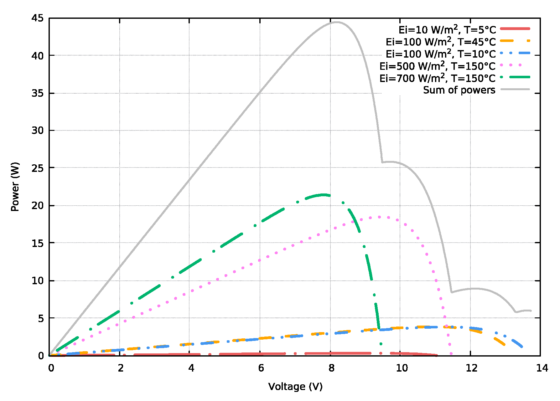
2.1.2. Design of Partial Shading Functions

The behavior that emulates a PV module or an array of PV modules under conditions of partial shading is achieved by simulating several modules, in our case 5, and applying variable values of irradiance and temperature in Equation (1). In this way, five partial functions were developed, which were subsequently added in order to obtain a test function necessary to evaluate the performance of numerical methods (See Figure 1).
Taking into account the number of curves in Figure 1, it is necessary to implement a method to unify the contributions of all functions in a single expression, maintaining the same structure for the four case studies in order to facilitate comparison between the optimization algorithms.
For this reason, an approach with artificial neural networks (ANN) was implemented because with the same architecture the approximation of the four case studies was carried out; which would not be achieved using polynomial approximation methods.
Figure 1 shows that the contribution of all PV modules generates several local maximums in the resulting function.

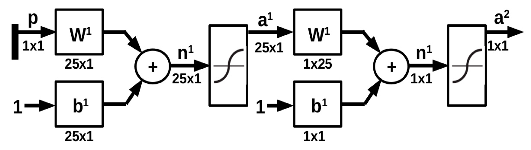
2.1.3. Architecture of the ANN Used for the Approximation

A feedforward neural network with a hidden layer, 25 neurons and an output layer with a neuron was implemented, as can be seen in Figure 2. All neurons have hyperbolic tangent sigmoid transfer function which is described in Equation (4). Initially, tests were carried out with 5 neurons but the results were not satisfactory, since the functions obtained presented problems at the inflection points. For this reason, it was decided to increase the number of neurons gradually until the best results were obtained with 25 neurons. Smoothed functions at the inflection points were obtained.
a = 2 ( 1 + e 2 n ) 1
This transfer function generates values in the interval [−1, 1].
To approximate each evaluation function, the architecture of the ANN is the same, only the synaptic weights and the bias change. To facilitate the training of the ANN, the data were normalized in a range of [−1, 1] (See Equation (5)). To revert this normalization, Equation (6) was used.
y = 2 ( x x m i n x m a x x m i n ) 1
y = 1 2 ( x + 1 ) ( x m a x x m i n ) + x m i n
where:
y is the output data,
x is the input data,
xmax: is the maximum value of the data to be evaluated,
xmin: is the minimum value of the data to be evaluated.
Finally, when xmax is equal to xmin, then y = x.
The networks were trained using the Matlab Neural Network Toolbox [32].

3. Numerical Optimization Algorithms

3.1. Golden Section Search Method

In this method, an interval is defined, and its regions are eliminated. For this, test points were added which allow new intervals to be formed. To choose the new extremes of the function, Equations (7) and (8) were used.
w 1 = a φ ( b a )
w 2 = b φ ( b a )
where: φ = 0.6180 and is described by the flowchart of Figure 3.
The flowchart begins with the initialization of the search range xl and xu, and the first solutions x1 and x2 are evaluated, where R is the golden number and C is its complement.

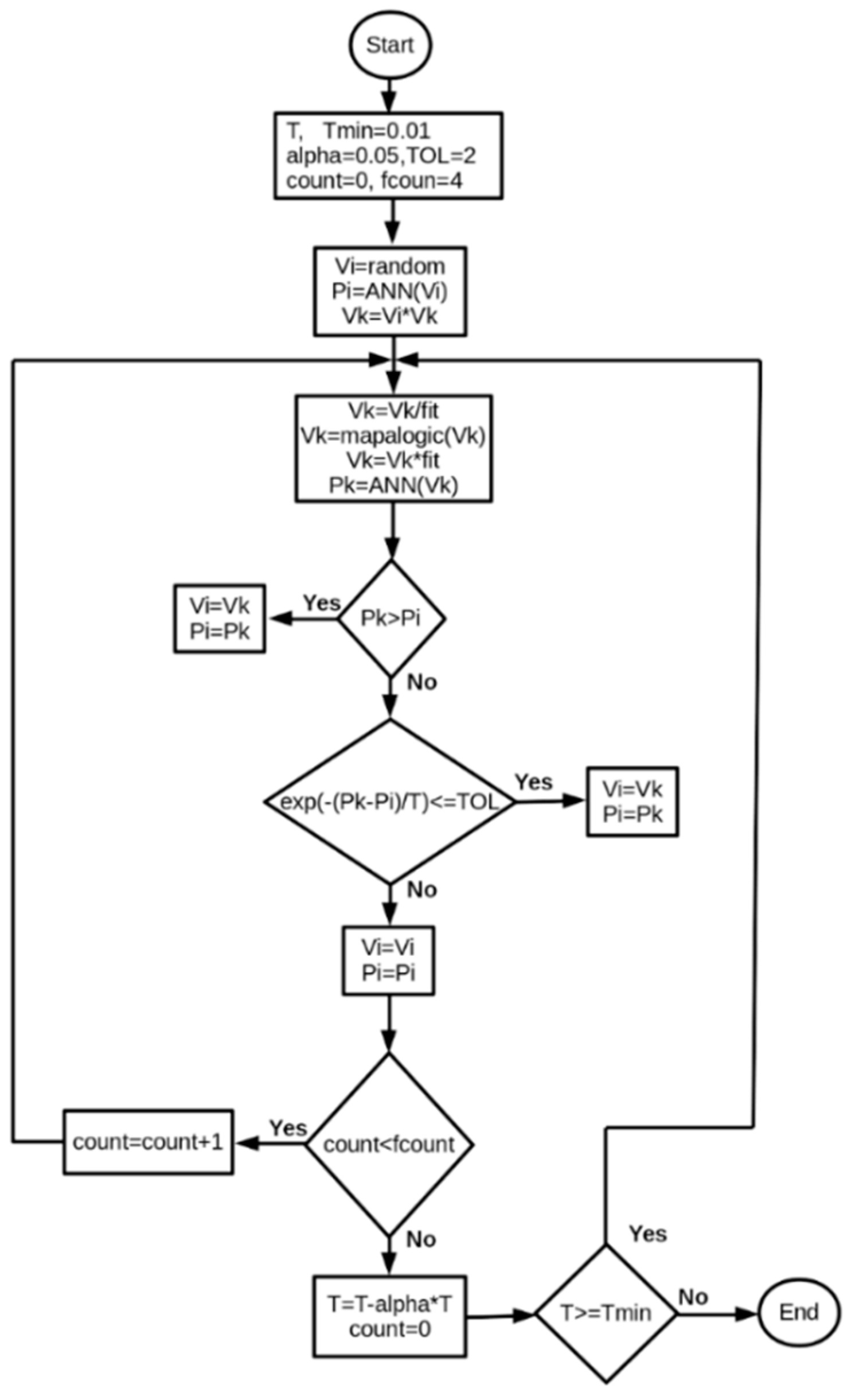
3.2. Simulated Annealing Algorithm

This algorithm is composed of two stochastic processes: One for the generation of solutions and another for the acceptance of that solutions, if they meet the criteria described in Equation (9), which is controlled by Equation (10). See Figure 4.
P e = e ( P k P i ) T
where:
Pe is the probability of acceptance,
Pk is the current maximum point,
Pi is the previous maximum point,
T is the computational temperature.
T ( n + 1 ) = T n α T n
where:
α is the cooling rate.

Logistics Map

The chaotic logistic map described in Equation (11) is implemented as a random function to generate possible solutions, in the simulated annealing algorithm.
x ( n + 1 )   =   r x n ( 1 x n )
where r is equal to 4.

4. Results and Discussion

The simulations of the algorithms were performed on a personal computer with a 64-bit Fedora 27 Workstation operating system, with Intel ® Core™ i3-3217U CPU @ 1.80 GHz and 4 GB of RAM. The compiler gcc version 7.3.1 20180712 (Red Hat 7.3.1-6) (GCC) was used. The codes were developed in C language and gnuplot was used to make the figures.

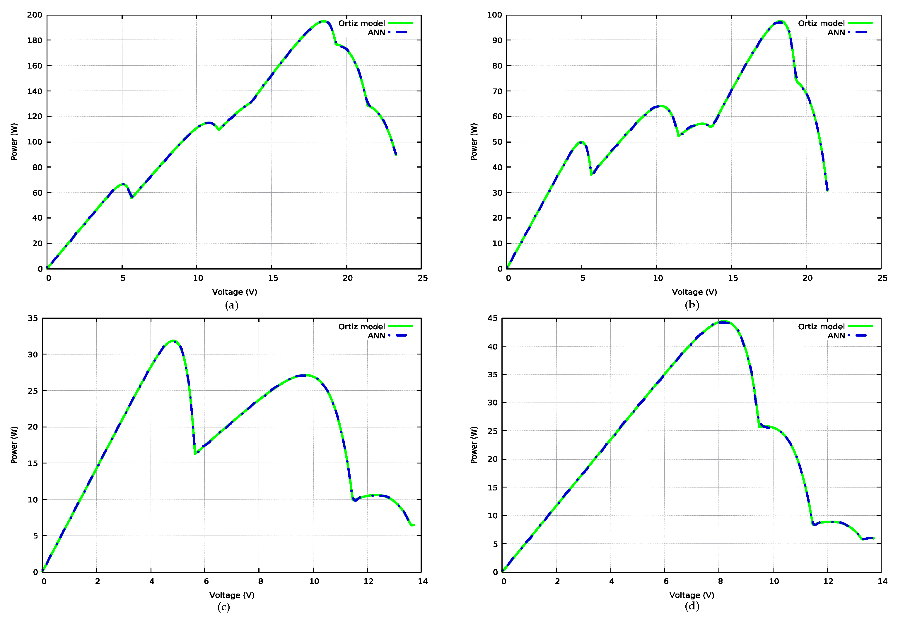
4.1. Approximation of the Test Functions with the Neural Network

This section presents the results obtained with the neural networks for the approximation of the evaluation functions generated by Equations (1)–(3).
In Table 1, it is shown that for most of the approximations the matrix R of the correlation coefficient is 1, which indicates a perfect correlation index, showing the good performance of the neural network.
Furthermore, in Figure 5, it is observed that the network suitably maps each of the functions. In some inflection points the network rounds a little more because the performance of a module or array of PV modules is simulated, the x-axis represents the voltage (volts) and the y-axis the power (watts).
All test functions have different characteristics, in order to evaluate algorithms in changing scenarios.
Table 2 shows the local maxima and the global maximum of each of the test functions, in which it can be established that the algorithms will be subjected to different challenges that emulate extreme operating conditions in the PV modules.

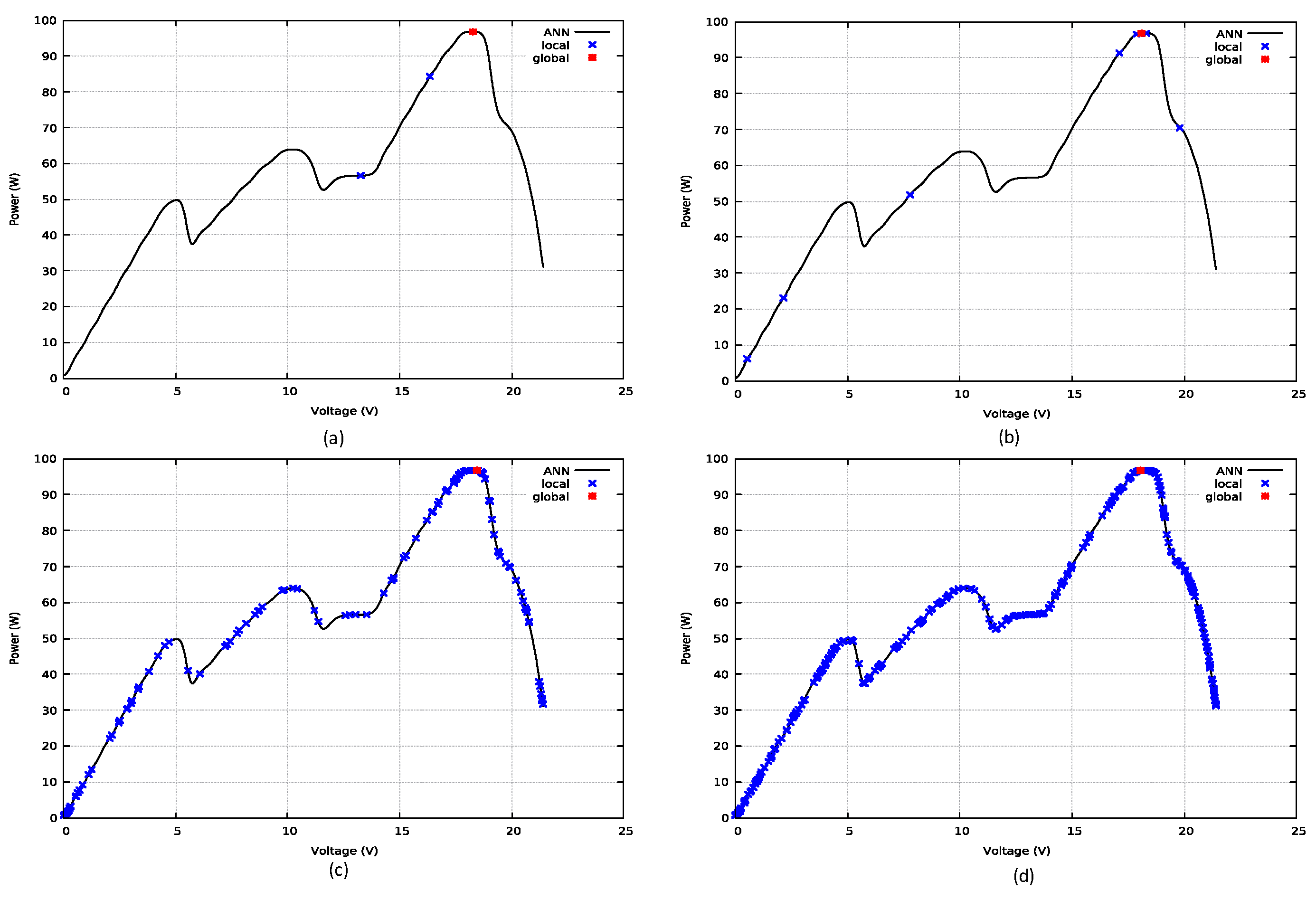
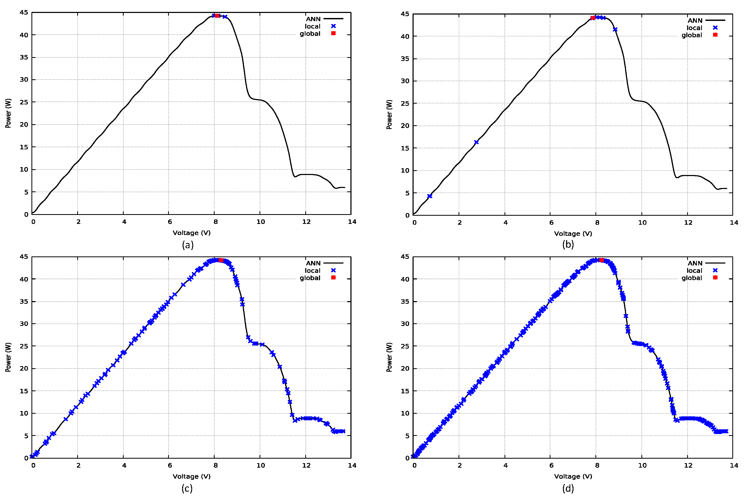
4.2. Results Obtained with Optimization Algorithms

In this section, the results of the optimization algorithms are shown, in terms of the maximum value found, the value evaluated in the function, the computation time and the number of iterations. In addition, a set of figures that show the partial solutions (in blue) and the global value found by the algorithms (in red) are presented. The solid black line is the test function.

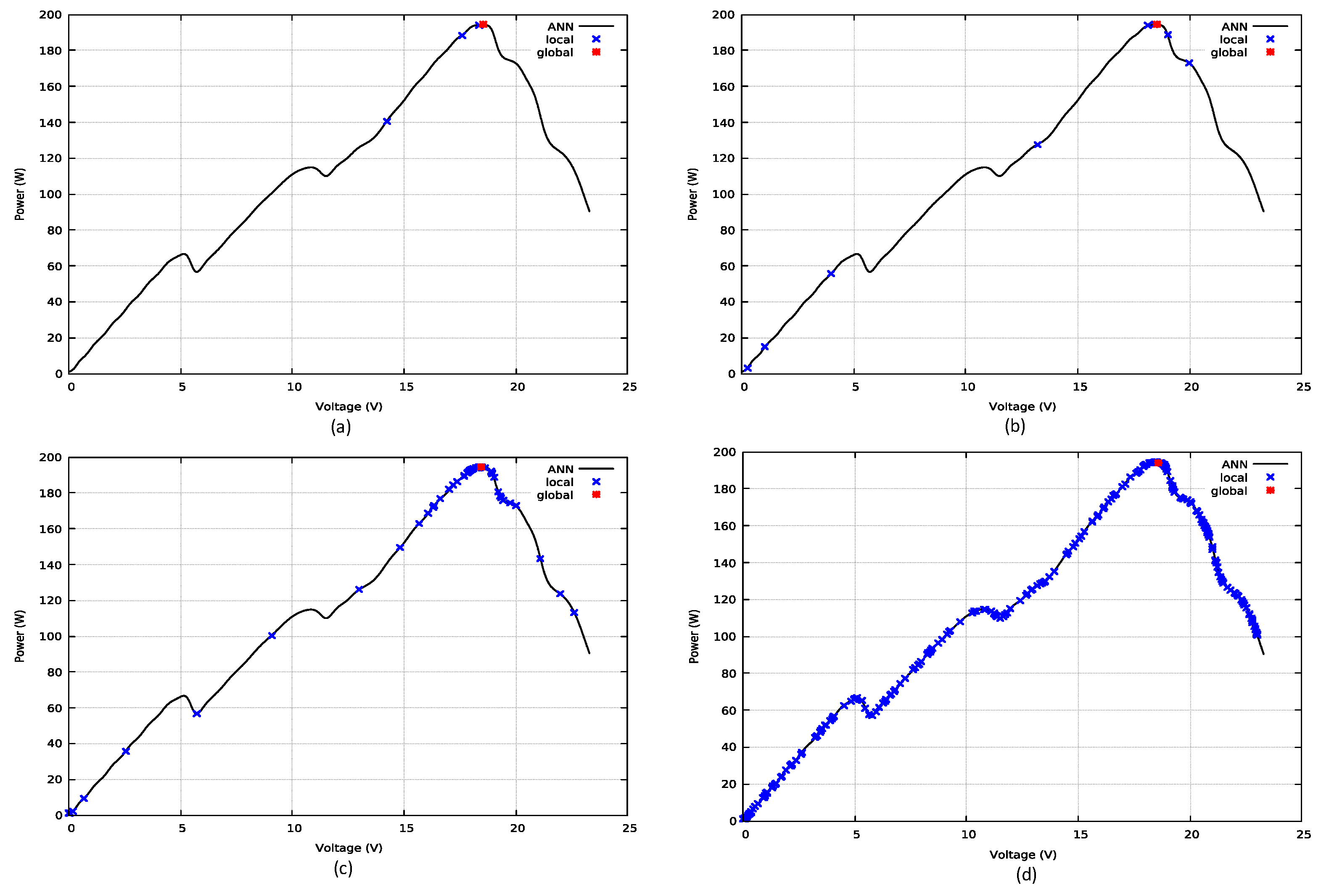
4.2.1. Results for Test Function 0

Table 3 shows the performance of the algorithms with the test function 0. The SA algorithm was implemented for initial temperatures of 0.5, 100 and 1000. In general, it can be seen that the algorithms find the global maximum, highlighting that, it has obtained a better computational efficiency with the GSS algorithm with a computation time of 0.189 ms and 9 iterations. In the case of the SA algorithm, it is observed that, with the increase of the initial temperature, the iterations increased from 160 to 900.
In addition, the GSS and SA (T = 0.5) algorithms presented the best error percentages of 0.14% and 0.13% for the component in x, and 0.02% and 0.03% for the component in f(x); with respect to the reference value of the global maximum.
Figure 6 shows the local maximums and the global maximum found by each of the algorithms. Figure 6c shows that the increase in the initial temperature causes the SA algorithm to perform a more exhaustive search, causing the number of local maxima to increase.

4.2.2. Results for Test Function 1

The results obtained for this case are shown in Table 4. The GSS algorithm presented a better computational time of 0.178 ms with only 8 iterations. This algorithm had the best error percentage with values of 0.03% and 0.44% for the components in x and f(x). It can also be observed that the increase in the initial temperature affects the performance of the SA algorithm, which presented errors of 0.81% and 0.54% (in x and f(x)) for T = 100.
Figure 7 shows the results obtained for this case. Variations in the global maximum found by each algorithm can be observed, as well as the increase in the number of iterations when the initial temperature increases.

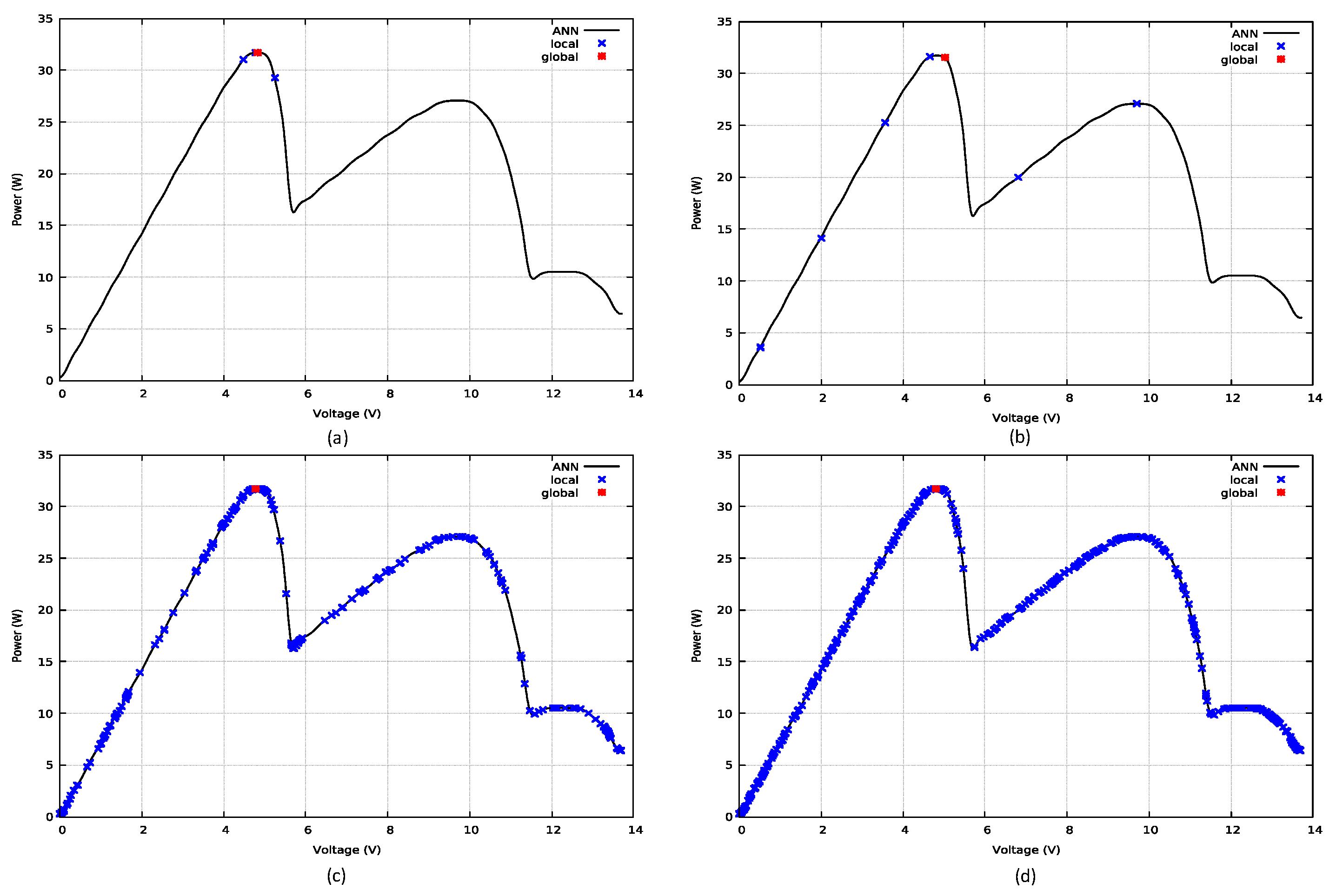
4.2.3. Results for Test Function 2

For this case, the results obtained are shown in Table 5. The analysis is similar to that performed for test function 1. The best performance (10 iterations and time of 0.188 ms) and percentage error (0.16% and 0.43%) was obtained with the GSS algorithm (See Figure 8).

4.2.4. Results for Test Function 3

Table 6 shows the results for test function 3. In this case, the SA algorithm with T = 1000 has the lowest error percentage with values of 0.66% and 0.26% for x and f(x). The GSS algorithm again has the best computational time (See Figure 9).

5. Conclusions

From the results obtained with the neural network, it can be concluded that it is important to have a universal structure to approximate the test functions, since a minimum variation in the computation times is achieved.
The choice of the range for the x-axis is an important factor that must be taken into account for the two algorithms implemented, golden section and simulated annealing. A bad choice of the range causes the algorithms to not find the global maximum.
On the other hand, the versatility of the simulated annealing algorithm is highlighted because the search mechanism can be controlled by adjusting the computational temperature and the cooling rate. The disadvantage is that many more iterations are performed and the search process becomes slower.
Another disadvantage of simulated annealing is that by having a larger group of possible solutions, some solution may be in the tolerance threshold and therefore accepted as the best option.
This research shows that with a single development of the algorithms several functions can be optimized, while with other methods such as neural networks it is necessary to adjust the synaptic weights and the bias. This same problem occurs with fuzzy logic, in which membership functions and fuzzy rules must be adjusted.

Author Contributions

J.G. and D.R.-L. performed the mathematical modeling and programming of numerical optimization algorithms. C.R.-A. and I.O. designed the experiments and wrote the manuscript.

Funding

This research was funded by Patrimonio Autónomo Fondo Nacional de Financiamiento para la Ciencia, la Tecnología y la Innovación Francisco José de Caldas, grant number 193-219 and the APC was funded by Vicerrectoría de Investigación of the Universidad del Magdalena.

Conflicts of Interest

The authors declare no conflict of interest.

References

  1. Chang, W.D. Multimodal function optimizations with multiple maximums and multiple minimums using an improved PSO algorithm. Appl. Soft. Comput. 2017, 60, 60–72. [Google Scholar] [CrossRef]
  2. Kaczmarczyk, V.; Bradac, Z.; Fiedler, P. A Heuristic Algorithm to Compute Multimodal Criterial Function Weights for Demand Management in Residential Areas. Energies 2017, 10, 1049. [Google Scholar] [CrossRef]
  3. Vieira, D.A.G.; Lisboa, A.C. Line search methods with guaranteed asymptotical convergence to an improving local optimum of multimodal functions. Eur. J. Oper. Res. 2014, 235, 38–46. [Google Scholar] [CrossRef]
  4. Tuo, S.; Zhang, J.; Yong, L.; Yuan, X.; Liu, B.; Xu, X.; Deng, F. A harmony search algorithm for high-dimensional multimodal optimization problems. Digit. Signal Process. 2015, 46, 151–163. [Google Scholar] [CrossRef]
  5. Thakur, M. A new genetic algorithm for global optimization of multimodal continuous functions. J. Comput. Sci. 2014, 5, 298–311. [Google Scholar] [CrossRef]
  6. Teo, J.C.; Tan, R.H.G.; Mok, V.H.; Ramachandaramurthy, V.K.; Tan, C. Impact of Partial Shading on the P-V Characteristics and the Maximum Power of a Photovoltaic String. Energies 2018, 11, 1860. [Google Scholar] [CrossRef]
  7. Bouselham, L.; Hajji, M.; Hajji, B.; Bouali, H. A New MPPT-based ANN for Photovoltaic System under Partial Shading Conditions. Energy. Proced. 2017, 111, 924–933. [Google Scholar] [CrossRef]
  8. Abu Eldahab, Y.E.; Saad, N.H.; Zekry, A. Enhancing the tracking techniques for the global maximum power point under partial shading conditions. Renew. Sustain. Energy Rev. 2017, 73, 1173–1183. [Google Scholar] [CrossRef]
  9. Li, G.; Jin, Y.; Akram, M.W.; Chen, X.; Ji, J. Application of bio-inspired algorithms in maximum power point tracking for PV systems under partial shading conditions. Renew. Sustain. Energy Rev. 2018, 81, 840–873. [Google Scholar] [CrossRef]
  10. Chaieb, H.; Sakly, A. A novel MPPT method for photovoltaic application under partial shaded conditions. Sol. Energy 2018, 159, 291–299. [Google Scholar] [CrossRef]
  11. Belhachat, F.; Larbes, C. Global maximum power point tracking based on ANFIS approach for PV array configurations under partial shading conditions. Renew. Sustain. Energy Rev. 2017, 77, 875–889. [Google Scholar] [CrossRef]
  12. Algarín, C.R.; Giraldo, J.T.; Álvarez, O.R. Fuzzy Logic Based MPPT Controller for a PV System. Energies 2017, 10, 2036. [Google Scholar] [CrossRef]
  13. Algarín, C.R.; Hernández, D.S.; Leal, D.R. A Low-Cost Maximum Power Point Tracking System Based on Neural Network Inverse Model Controller. Electronics 2018, 7, 4. [Google Scholar] [CrossRef]
  14. Viloria-Porto, J.; Robles-Algarín, C.; Restrepo-Leal, D. A novel approach for an MPPT controller based on the ADALine network trained with the RTRL algorithm. Energies 2018, 11, 3407. [Google Scholar] [CrossRef]
  15. Kheldoun, A.; Bradai, R.; Boukenoui, R.; Mellit, A. A new Golden Section method-based maximum power point tracking algorithm for photovoltaic systems. Energy Convers. Manag. 2016, 111, 125–136. [Google Scholar] [CrossRef]
  16. Gayathri, R.; Ezhilarasi, G.A. Golden section search based maximum power point tracking strategy for a dual output DC-DC converter. Ain Shams Eng. J. 2017, 9, 2617–2630. [Google Scholar] [CrossRef]
  17. Chaves, E.N.; Reis, J.H.; Coelho, E.A.A.; Freitas, L.C.G.; Júnior, J.B.V.; Freitas, L.C. Simulated Annealing MPPT in Partially Shaded PV Systems. IEEE. Lat. Am. Trans. 2016, 14, 235–241. [Google Scholar] [CrossRef]
  18. Lyden, S.; Haque, M.E. A Simulated Annealing Global Maximum Power Point Tracking Approach for PV Modules under Partial Shading Conditions. IEEE. Trans. Power. Electron. 2016, 31, 4171–4181. [Google Scholar] [CrossRef]
  19. Rahmat, M.K.; Jovanovic, S.; Lo, K.L. Reliability and Availability Modelling of Uninterruptible Power Supply Systems Using Monte-Carlo Simulation. Int. J. Energy Convers. 2017, 5, 60–66. [Google Scholar] [CrossRef]
  20. Passino, K.M.; Yurkovich, S. Fuzzy Control; Addison-Wesley: Menlo Park, CA, USA, 1997; pp. 23–51. [Google Scholar]
  21. Hagan, M.T.; Demuth, H.B.; Beale, M.H.; De Jesús, O. Neural Network Design, 2nd ed.; Oklahoma State University: Stillwater, OK, USA, 2014; pp. 36–50. [Google Scholar]
  22. Haykin, S. Neural Networks: A Comprehensive Foundation, 2nd ed.; Prentice Hall: Upper Saddle River, NJ, USA, 1998; pp. 23–28. [Google Scholar]
  23. Hen Hu, Y.; Hwang, J.-N. Handbook of Neural Network Signal Processing; CRC Press LLC: Boca Raton, FL, USA, 2002; pp. 42–45. [Google Scholar]
  24. Wang, G.; Tan, Z.; Tan, Q.; Yang, S.; Lin, H.; Ji, X.; Gejirifu, D.; Song, X. Multi-objective robust scheduling optimization model of wind, photovoltaic power, and bess based on the Pareto principle. Sustainability 2019, 11, 305. [Google Scholar] [CrossRef]
  25. Nasirudin, A.; Chao, R.-M.; Utama, I.K.A.P. Solar powered boat design optimization. Procedia Eng. 2017, 194, 260–267. [Google Scholar] [CrossRef]
  26. Ozgonenel, O.; Karagol, S.; Terzi, U.K. A novel approach for distributed renewable generation and shunt capacitor placing in smart-grid. IEEE Pes. Innov. Smart 2015, 2015, 7028983. [Google Scholar] [CrossRef]
  27. Khanjarpanah, H.; Jabbarzadeh, A. Sustainable wind plant location optimization using fuzzy cross-efficiency data envelopment analysis. Energy 2019, 170, 1004–1018. [Google Scholar] [CrossRef]
  28. Zhang, W.; Maleki, A.; Rosen, M.A.; Liu, J. Sizing a stand-alone solar-wind-hydrogen energy system using weather forecasting and a hybrid search optimization algorithm. Energy Convers. Manag. Energy 2019, 180, 609–621. [Google Scholar] [CrossRef]
  29. Malathy, S.; Ramaprabha, R. A two-stage tracking algorithm for PV systems subjected to partial shading conditions. Int. J. Renew. Energy Res. 2018, 8, 2249–2256. [Google Scholar]
  30. Wang, F.; Zhu, T.; Zhuo, F.; Yi, H.; Fan, Y. Enhanced simulated annealing-based global MPPT for different PV systems in mismatched conditions. J. Power Electron. 2017, 17, 1327–1337. [Google Scholar] [CrossRef]
  31. Lyden, S.; Haque, M.E. A comprehensive study of the key parameters of the Simulated Annealing method for maximum power point tracking in photovoltaic systems. In Proceedings of the IEEE Power and Energy Society General Meeting, Boston, MA, USA, 17–21 July 2016; Volume 2016, p. 7741788. [Google Scholar] [CrossRef]
  32. Demuth, H.B.; Hagan, M.T.; Beale, M.H. Neural Network Toolbox User’s Guide R2013b; The MathWorks, Inc.: Natick, MA, USA, 2013; pp. 129–188. [Google Scholar]
Figure 1. Sum of powers.
Computation 07 00043 g001
Figure 2. Artificial neural networks (ANN) feedforward.
Computation 07 00043 g002
Figure 3. Flowchart of the golden section method.
Computation 07 00043 g003
Figure 4. Flowchart of the simulated annealing algorithm.
Computation 07 00043 g004
Figure 5. Test functions generated with the neural network: (a) Function 0; (b) Function 1; (c) Function 2; (d) Function 3.
Computation 07 00043 g005
Figure 6. Results obtained with the algorithms for the test function 0: (a) GSS; (b) SA (T = 0.5); (c) SA (T = 100); (d) SA (T = 1000).
Computation 07 00043 g006
Figure 7. Results obtained with the algorithms for the test function 1: (a) GSS; (b) SA (T = 0.5); (c) SA (T = 100); (d) SA (T = 1000).
Computation 07 00043 g007
Figure 8. Results obtained with the algorithms for the test function 2: (a) GSS; (b) SA (T = 0.5); (c) SA (T = 100); (d) SA (T = 1000).
Computation 07 00043 g008
Figure 9. Results obtained with the algorithms for the test function 3: (a) GSS; (b) SA (T = 0.5); (c) SA (T = 100); (d) SA (T = 1000).
Computation 07 00043 g009
Table 1. Correlation coefficients obtained for the test functions.
Test FunctionsR
Function 0 1  
Function 1 0.99  
Function 2 1  
Function 3 1  
Table 2. Maximum points of the test functions.
Test FunctionsLocal MaximumsGlobal Maximum
Function 0[5.11, 66.19], [10.76, 114.72][18.5056, 194.412]
Function 1[4.97, 49.74], [10.33, 64.13], [13.06, 57.02][18.2847, 97.3037]
Function 2[9.82, 27.12], [12.46, 10.60][4.82874, 31.8543]
Function 3[9.82, 25.73], [12.31, 8.80][8.19883, 44.2902]
Table 3. Results of the algorithms for the test function 0.
ComponentsGSSErrorSA T = 0.5ErrorSA T = 100ErrorSA T = 1000Error
x18.4791620.14%18.5300240.13%18.4655740.22%18.5753420.37%
gf(x)194.3703310.02%194.3576050.03%194.3700870.02%194.3247680.04%
Time (ms)0.189 2.175 7.904 10.585
Iterations9 160 675 900
Table 4. Results of the algorithms for the test function 1.
ComponentsGSSErrorSA T = 0.5ErrorSA T = 100ErrorSA T = 1000Error
x18.2792420.03%18.3960320.61%18.4331000.81%18.0351011.36%
f(x)96.8714600.44%96.8125310.50%96.7761380.54%96.8011550.52%
Time (ms)0.178 2.514 8.113 9.580
Iterations8 160 675 900
Table 5. Results of the algorithms for the test function 2.
ComponentsGSSErrorSA T = 0.5ErrorSA T = 100ErrorSA T = 1000Error
x4.8363980.16%5.0195493.95%4.7803781.00%4.7929310.74%
f(x)31.7157710.43%31.5061041.09%31.7076820.46%31.7113510.45%
Time (ms)0.188 1.429 4.046 5.41
Iterations10 160 675 900
Table 6. Results of the algorithms for the test function 3.
ComponentsGSSErrorSA T = 0.5ErrorSA T = 100ErrorSA T = 1000Error
x8.1106841.08%7.8644484.08%8.4325902.85%8.2528930.66%
f(x)44.1965260.21%44.0637970.51%44.0389750.57%44.1734160.26%
Time (ms)0.280 2.018 4.019 8.82
Iterations9 160 675 900

