Article

Aerodynamic Optimization of Airfoil Profiles for Small Horizontal Axis Wind Turbines

by
Ali Cemal Benim
1,2,*,
Michael Diederich
1 and
Björn Pfeiffelmann
1
1
Center of Flow Simulation (CFS), Department of Mechanical and Process Engineering, Düsseldorf University of Applied Sciences, Münsterstr. 156, D-40476 Germany
2
Institute of Thermal Power Engineering, Department of Mechanical Engineering, Cracow University of Technology, Al. Jana Pawła II 37, 31-864 Kraków, Poland
*
Author to whom correspondence should be addressed.
Computation 2018, 6(2), 34; https://doi.org/10.3390/computation6020034
Submission received: 2 March 2018 / Revised: 19 April 2018 / Accepted: 21 April 2018 / Published: 25 April 2018
(This article belongs to the Special Issue Computational Methods in Wind Engineering)

Abstract

:
The purpose of this study is the development of an automated two-dimensional airfoil shape optimization procedure for small horizontal axis wind turbines (HAWT), with an emphasis on high thrust and aerodynamically stable performance. The procedure combines the Computational Fluid Dynamics (CFD) analysis with the Response Surface Methodology (RSM), the Biobjective Mesh Adaptive Direct Search (BiMADS) optimization algorithm and an automatic geometry and mesh generation tool. In CFD analysis, a Reynolds Averaged Numerical Simulation (RANS) is applied in combination with a two-equation turbulence model. For describing the system behaviour under alternating wind conditions, a number of CFD 2D-RANS-Simulations with varying Reynolds numbers and wind angles are performed. The number of cases is reduced by the use of RSM. In the analysis, an emphasis is placed upon the role of the blade-to-blade interaction. The average and the standard deviation of the thrust are optimized by a derivative-free optimization algorithm to define a Pareto optimal set, using the BiMADS algorithm. The results show that improvements in the performance can be achieved by modifications of the blade shape and the present procedure can be used as an effective tool for blade shape optimization.

1. Introduction

Wind power has been receiving increasing attention as one of the most promising renewable energy sources. Wind turbine technologies for improved performance have been developed within the last two decades, where many aspects, including aerodynamics and aeroelasiticy, have been the subject of intensive theoretical, computational and experimental research [1]. As the airfoil profile shape has a crucial impact on the aerodynamic efficiency of a wind turbine, an important research area for wind turbine technology has been blade design. Within this context, automatic blade shape optimization procedures, which have a longer tradition in other areas such as compressors [2] and turbines [3] have also been used for the aerodynamic and structural optimization of wind turbine blades. The more classical intuition and experience based non-automatic optimization [4] has been used. In our study, we focus on Horizontal Axis Wind Turbines (HAWT).
Jureczko et al. [5] applied a genetic algorithm (GA) to optimize wind turbine blades, where the emphasis was put on structural stability. The aerodynamic loads were calculated by the Blade Element Momentum (BEM) theory. Genetic algorithms along with the BEM theory were used also by Mendez and Greiner [6] for aerodynamic optimization with respect to blade chord and twist angle. Burger and Hartfield [7] examined the feasibility of using the combination of the vortex lattice method with a GA for the optimization of the aerodynamic performance of horizontal axis wind turbine blades. Clifton-Smith and Wood [8] applied differential evolution strategies to optimize numerically small wind turbine blades with the double purpose of maximizing power coefficient and minimizing starting time. Here, the power coefficient was calculated by the standard BEM theory.
Liu et al. [9] developed an optimization model based on an extended compact genetic algorithm to maximize the annual energy output of a 1.3 MW stall-regulated wind turbine. The flow field was computed by the XFOIL code [10], which is based on an inviscid linear-vorticity panel method, which can take viscous effects by superimposed sources into account. Compared to the original blades, the designed blades showed better aerodynamic performance.
A multidisciplinary design approach along with a gradient based optimization algorithm was used to solve the optimization problem of a wind turbine blade by Kenway and Martins [11]. The blade aerodynamics was modelled by the BEM theory. The blade was constructed using 7 design variables: chord, twist, spar (thickness, location and length), airfoil thickness and rotation rate. To demonstrate the potential for site-specific optimization, a 5 kW wind turbine case was used with results showing a possible output increase of 3–4%. In the analysis by Xudong et al. [12], the costs were also considered along with the aerodynamic/aeroelastic model and the cost of energy based on annual energy production was minimized, where the aerodynamic model was based on the BEM theory. Ceyhan et al. [13] studied the aerodynamic performance of horizontal axis wind turbine blades using the BEM theory and GA. The fitness function was based on the BEM theory, where two design variables, the chord and twist distributions, were optimized for optimum power production. An increase of 40–80% in power production was recorded on a 100 kW HAWT.
Li et al. [14] presented an improved optimization technique using response surface methods to optimize the lift-to-drag ratio for 2D wind turbine airfoils. Grujicic et al. [15] developed a two-level optimization scheme consisting of an inner and outer level. In the inner level, for a given aerodynamic design of the blade, which was based on a CFD analysis, the blade mass was minimized. Bottasso et al. [16] applied a complex multi-disciplinary approach for optimally sizing large, multi-MW wind turbines, seeking a compromise between the maximization of the annual energy production and the weight of the machine, assuming the weight is well correlated with the cost. The multi objective design is not formulated as a Pareto optimal problem but rather as a combined cost problem defined as the ratio of the annual energy production to the total weight.
An approach to optimizing the power factor and the power output of the wind turbine (bi-objective problem established by weights) using data-mining and evolutionary computation was presented by Kusiak and Zheng [17]. Song et al. [18] developed a MATLAB tool using BEM theory to perform aerostructural dynamic analysis of wind turbine blades on a 20 kW wind turbine. These authors optimized the chord length and twist angle at each blade element to maximize the wind energy utilization factor of each blade element. Wang et al. [19] presented a multi-objective algorithm where the maximum power coefficient at the design wind speed (9 m/s) and the minimum blade mass were chosen as two optimization objectives; a conflicting problem. The aerodynamic loads acting on the blade were calculated using the modified BEM theory.
Later in 2012, Graaso [20] focused on the airfoil design at the tip region of the blade using numerical optimization. Genetic and gradient based algorithms were used, on a hybrid optimization platform, to design a new family of airfoils dedicated to the root region of the wind turbine blade. This approach improved aerodynamic efficiency (lift-to-drag ratio) together with the sectional moment of resistance for the structural part of the problem. The flow was computed by the XFOIL code.
Chen and Agarwal [21] applied a GA for shape optimization of flatback airfoils, which was enhanced by combination with an artificial neural network algorithm. A considerable acceleration of the procedure by the use of artificial neural networks was reported, without, however, a quantification. For calculating the flow field, a CFD approach was employed. Ribeiro et al. [22] coupled CFD based flow analysis with an optimization algorithm for wind turbine airfoil design. Single and multi-objective GA were employed and artificial neural networks were used as a surrogate model. In the study, the effect of the domain size on the prediction and the effect of parallelization on speed-up were discussed. The use of artificial neural networks was shown to reduce the computational time by almost 50%.
Jeong et al. [23] minimized the fluctuations of the unsteady aerodynamic load under turbulent wind conditions. It was noted that the out-of-plane fluctuating unsteady aerodynamic load is more significant than the in-plane loads for structural fatigue of the blade. The RMS out-of-plane bending moment was reduced by about 20% and its mean was reduced by about 5%. Semi-empirical methods were used to estimate the sound pressure.
Ju et al. [24] developed a robust design optimization procedure for wind turbine airfoils by maximizing the lift to drag coefficient ratio and the lift coefficients of the airfoil, along with a sensitivity minimization of the roughness at the leading edge associated with the geometry profile uncertainty. The flow field information was obtained by a CFD approach.
The optimization of spar caps in wind turbine blades was examined by Liao et al. [25]. The thickness and the location of spars were chosen as the optimization variables. The FAST aero-elastic simulator was used along with unsteady BEM. Polat and Tuncer [26] optimized blade shapes for the maximization of power production at a specific wind speed, rotor speed and rotor diameter, applying a GA, within the framework of a parallel computing environment, using XFOIL as the flow solver.
Sessarego el al. [27] performed the multi-objective optimization of wind-turbine blades using a non-dominated sorting genetic algorithm. Annual energy production, flapwise root-bending moment and the mass of the turbine blade were considered as the objective functions. The aerodynamic model was based on BEM. Shen et al. [28] performed a multi-objective optimization of wind turbine blades using the lifting surface method as the aerodynamic model. Maximization of annual energy production and minimization of blade load including thrust and blade flap-wise moment were considered as the objective functions.
Hassanazadeh et al. [29] carried out the aerodynamic shape optimization and the analysis of small wind turbine blades using BEM and GA. Annual energy production was considered as the objective function. Porrajabian et al. [30] performed the aero-structural design optimization of a small wind turbine. Starting time of turbine and output power were considered simultaneously as the objective function. The design variables consisted of the chord, twist and the shell thickness. The aerodynamic model was based on the BEM theory. Dal Monte et al. [31] presented a procedure for aerodynamic-structural optimization of wind turbine blades, where the structural modelling was based on the finite element method and the aerodynamic part was based on the BEM theory. A more detailed survey of performance optimization techniques applied to wind turbines is presented in a recent review by Chehouri et al. [32].
Inspecting the previous work on the automatic optimization of wind turbine blade shapes, one can see that aerodynamic analysis has been most frequently based on the BEM method but rarely on the solution of the Navier-Stokes equations via CFD. Thus, a distinguishing feature of the present contribution from the majority of the previous work is the CFD based analysis of the flow field. In previous work on the automated optimization of wind turbine blade shapes, CFD based flow analysis was also reported by Bottasso et al. [16], Li et al. [14], Chen and Agarwal [21], Riberio et al. [22], Ju and Zhang [24]. Bottasso et al. [16] presented the applied the multi-disciplinary constrained optimization, however, hardy provided any detail information on the structural or flow (CFD) analysis. Li et al. [14] applied a CFD approach for the aerodynamic analysis. However, many details of the applied models and methods such as the turbulence model, discretization schemes were not provided and a grid independence study was not performed. In the work of Chen and Agarwal [21] a grid independence study was performed and the applied turbulence model was discussed. However, in conjunction with the latter, some important details are not sufficiently addressed such as the near-wall treatment that is crucial for prediction of the boundary layer development and flow separation.
Riberio et al. [22] and Ju and Zhang [24] presented a more detailed CFD analysis, where the details of the mathematical and numerical formulation were adequately addressed. A difference of the present mathematical CFD formulation compared to those of Riberio et al. [22] and Ju and Zhang [24] resides in the applied turbulence model. In [22,24] a one-equation turbulence model was used, where in the present study a principally more accurate two-equation turbulence model is employed. Furthermore, in References [22,24] only the angle of attack (AoA) was varied, while the approach velocity magnitude was kept constant. In the present study, the flow angle (FA) for the prevailing blade angle (BA) and the magnitude of the approach velocity, that is, the Reynolds number are varied independently from each other, which span a higher dimensional space from which an optimal blade shape is sought. Here, BA is the angle between the blade chord and the plane of rotation and FA is the angle between relative approach velocity vector and the plane of rotation (obviously the AoA results from the FA for a given BA). Considerable variations of FA are quite likely for small HAWT, as many of them use furling, whereby the rotor yaws out of the wind as a measure of protection against overspeed. In the previous studies [14,21,22,24], an essentially infinite domain size was considered, whereas in the present work, the effect of the domain size and the blade-to-blade interaction are addressed.
There are also differences in the applied optimization methods between the present and previous studies. In [14] the Response Surface Methodology (RSM) [33] was used as the optimization method. In [21,22,24] GA enhanced with artificial neural networks were used as the optimization procedure. In the present work the RSM is used to describe the effect of flow variables for the unmodified blade shape, which was an input for the subsequent optimization. The optimization of the blade shape was performed by a Biobjective Mesh Adaptive Direct Search (BiMADS) optimization algorithm. Furthermore, beyond high trust, a stable performance under varying wind conditions is considered as an additional goal within the present bi-objective optimization, whereas the latter objective was not addressed in the previous, comparable investigations.

2. Model Description

2.1. Overview of the Optimization Procedure

The optimization cycle is depicted in Figure 1. The blade shape is represented by a finite number of degrees of freedom (to be described, below, in more detail). They are denoted as “geometry parameters” in Figure 1. The optimization cycle is started by the optimization algorithm, which generates the geometry parameters and transfers them to the mesh generator to create a CFD grid. At the first cycle, the geometry parameters are, however, not generated by the optimization algorithm but stem from the original geometry. The Response Surface Methodology (RSM) module defines the aerodynamic operation points according to certain rules (to be defined later in more detail) that are fed to the computational flow solver (CFD) as boundary conditions, together with the computational mesh. Based on the CFD results, two values are calculated and passed over to the optimization module by the RSM module. These are the average thrust, that is, the tangential force (the force component in the direction of rotation that generates the power) and its standard deviation within the considered space of flow variables. The maximization of the former (maximum power) and the minimization of the latter are the objective functions (efficient and stable operation under varying wind conditions). The optimization algorithm (to be described later in more detail) proposes a new set of geometry parameters for the better fulfilment of these objectives, which closes the cycle.

2.2. Mathematical and Numerical Modelling of the Aerodynamics

The flow is assumed to be two-dimensional (2D) and statistically in the steady state. For a rotating turbine with fixed blades, this setting resembles a blade-to-blade surface at a fixed radial section, where the turbine rotational speed and the wind speed are constant in time, in a moving (i.e., rotating) reference frame. In the sense of a quasi-three dimensional procedure, which is also quite common in steam [34] and gas [35] turbines, a three-dimensional model can be constructed by an assembly of such blade-to-blade sections. It shall be noted that the resemblance is, however, approximate in so far, that a curved blade-to-blade surface resulting from a radial section is represented by a flat plane in 2D. The air flow is assumed to be incompressible, which is reasonable at the usually prevailing Mach numbers in HAWT applications. The Navier-Stokes equations along with the continuity equation are solved computationally.
The Computational Fluid Dynamics (CFD) analysis is based on the general-purpose code CFD ANSYS Fluent [36], applying the Finite Volume Method (FVM) for discretizing the governing differential equations. Flow turbulence is modelled within a RANS (Reynolds Averaged Numerical Simulation) approach [37], where the time-averaged equations are solved for the time-averaged variables in steady-state. A more accurate approach would be Large Eddy Simulations (LES) [38,39], which, being a three-dimensional and unsteady approach, would, however explode the frame in the present case. Turbulence is modelled by a two-equation turbulence model, that is, by the Shear Stress Transport (SST) model [36,40], which were shown to perform quite reliably especially for wall-driven turbulent flows with potential to predict transitional effects [41,42,43]. No wall-functions are used near the wall, resolving the near-wall layer. The coupling of the discretized Navier-Stokes and continuity equations are treated by a coupled solver [36,44]. The convective terms are discretized by a formally third-order accurate QUICK discretization scheme [36,45] for the Navier-Stokes equations and a second-order upwind scheme [36,46] for the transport equations of the two turbulence variables. Convergence criterion for the residual of each equation was set to 10−5.

2.3. Flow Solution Domain and Boundary Conditions

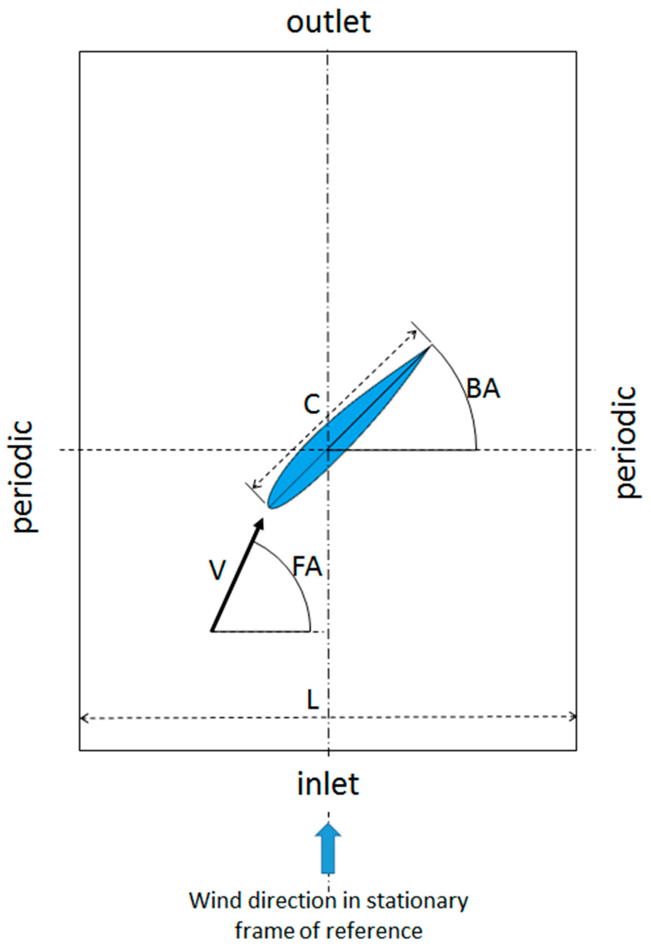
The airfoil is positioned in a rectangular domain, with periodic boundaries on both sides in the circumferential direction, along with an inlet and an outlet boundary. The solution domain and the boundary definitions are sketched in Figure 2, where the velocity vector relative to the airfoil, the flow angle (FA) and blade angle (BA) are also indicated.
The inlet and outlet boundaries are placed ten and twenty chord lengths (C) away from the airfoil, respectively, which may be considered to be sufficiently far [47] that the boundaries do not influence the results. At the inlet, uniform distributions of the velocity components (the approach velocity V relative to the airfoil, Figure 2) and turbulence quantities are prescribed. The inlet values of the turbulence quantities are estimated assuming a turbulence intensity of 4% and a macro-mixing length [37] of 25% of the chord length. At the outlet, a constant static pressure is prescribed along with zero-gradient conditions for the remaining quantities. At the pair of periodic boundaries, obviously, periodic boundary conditions are applied. The extension of the domain between the two periodic boundaries (L) corresponds to the space between two neighbouring blades in a turbine wheel. In an application, in general, this size varies with the number of blades on the wheel, as well as the radial position of the considered blade-to-blade section.

2.4. Generation of Computational Grid for Flow Simulation

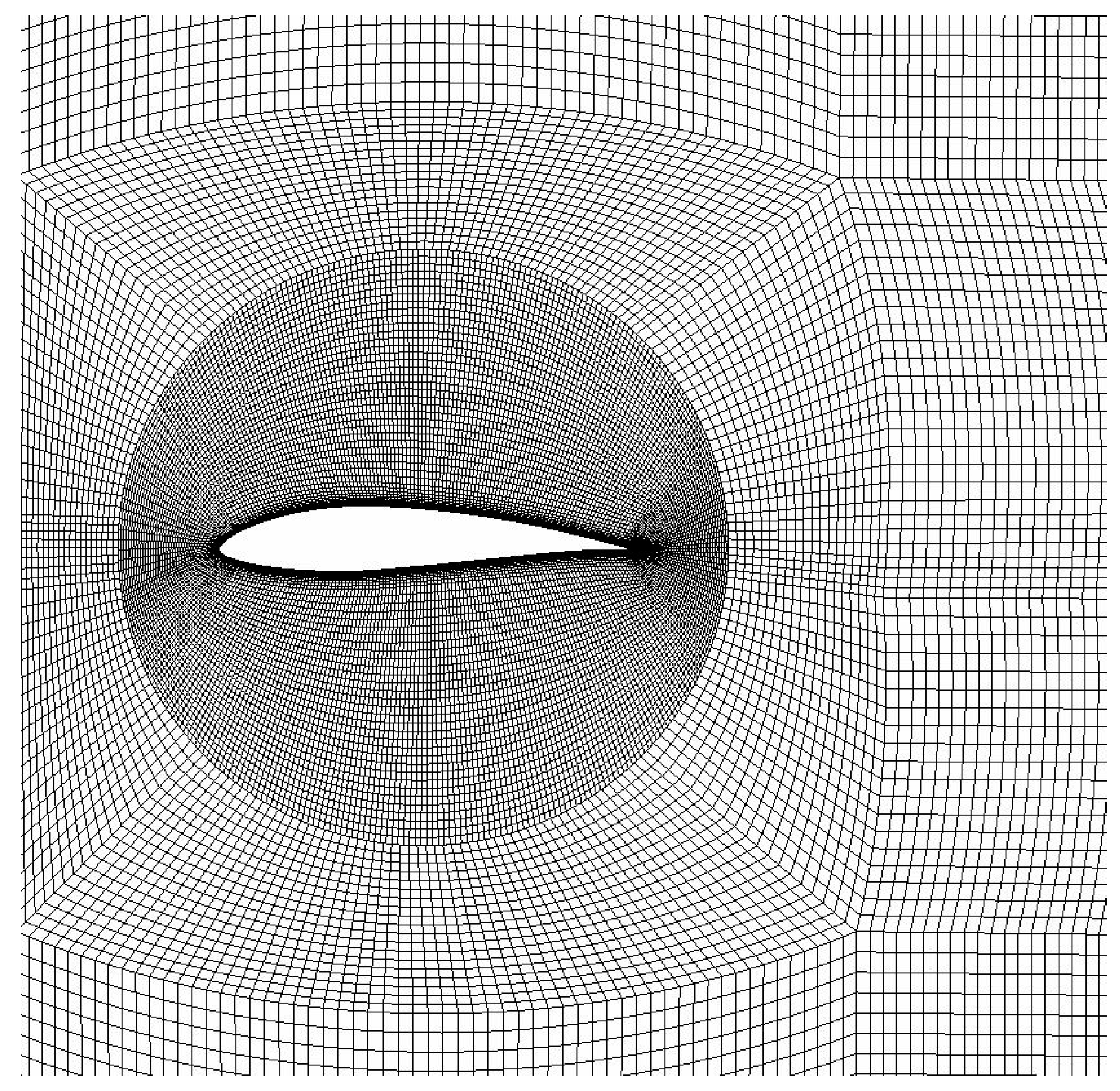
A high-quality O-grid is generated around the blade, which interfaces with the essentially H-type block-structured grid in the outer domain. Via an in-house developed procedure based on the ANSYS ICEM grid generator [36] and replay scripts, different grids for different blade positions and different blade surface shapes can automatically be generated. Prompted by the optimization algorithm by the transfer of the geometry controlling parameters, the mesh generation module calculates the Hermite curves, manipulates the replay script (which stems from the previous grid) accordingly and prompts the ANSYS ICEM grid generator to generate the new mesh with the new replay script and transfers the mesh to the RSM module (Figure 1). These processes are controlled by scripts written in GNU Octave [48]. Since no-wall functions for turbulence modelling have been used, the grid resolution near the wall needs to be sufficiently fine. In generating the grids, it is ensured that the non-dimensional wall-distance y+ [37] is everywhere smaller than 1 for the next-to-wall cells and at least 3 cells remain within the region y+ < 5. The structure of a typical grid is displayed in Figure 3. From case-to-case, changes in the grid are confined to the O-grid surrounding the airfoil. The variations in the airfoil profile cause a grid modification only in this region and different BA can be obtained by the respective rotations of the O-grid connected to the airfoil.

2.5. Parametrization of the Airfoil Shape

For the optimization, the airfoil geometry needs to be parametrized. Historically, different approaches have been used. For the present purposes, the Hermite curves, which are closely related with Bezier curves, are found to be most suitable for generating airfoil shapes with a limited number of parameters and with sufficient geometrical precision. A Hermite curve is defined by two points (Pi) and two tangent vectors (with lengths lij and directions αi) on both its ends. With this function, the geometry of the airfoils has been generated by using four piecewise Hermite curves (HCi), two representing the suction and two the pressure side, as shown in Figure 4.
The Hermite curve segments are connected with each other in a continuous fashion at points P2, P3, P4 by ensuring that the end-point of one curve is the same as the starting point of another and the local tangent vectors belonging to the curves that are joined at this point have the same direction for ensuring C1 continuity. The mathematical expression of the Hermite curve i (HCi), bounded by points Pi and Pj (with j = I + 1), is provided below (Figure 4).
x i ( t ) = ( P i + 3 P I i i 3 P I j i + P j )    t 3 + ( 3 P i 6 P I i i + 3 P I j i )    t 2 + ( 3 P i + 3 P I i i )    t + P i
where the vector x i contains the coordinate pair of any point on the curve HCi, the variable t is a parameter varying along the curve between 0 (at Pi) and 1 (at Pj) and
P I i i = P i + e l l ( α i )    l i i ; P I j i = P j + e l l ( α i ) l j i
with e l l ( α i ) denoting the unit direction vectors along tangents, pointing away from the corresponding edge points.
Assuming production by glass fibre-reinforced synthetic material moulding, a trailing edge with finite thickness is considered, which is defined by points P1 and P5 that are connected by a tiny straight line. In addition to the coordinates of the five points, the directions of the vector couples as well as their lengths describe the shape of the airfoil. The number of degrees of freedom can be reduced by introducing certain constrains on these parameters, which will be addressed below.

2.6. Response Surface Methodology and the Optimization Algorithm

Response Surface Methodology (RSM) [33] is a general approach to describe the response of certain output variables to the changes in the independent variables, that is, the influencing variables. For a well distributed number of “design points” in the space of the independent variables, a regression function, that is, an objective function, is created using the least-square approach, which can be used as basis for different optimization purposes. RSM can be used as an optimization scheme of its own [14]. However, in the present case, with a quite large number of influencing variables (when the airfoil shape parameters are also covered by the regression function), this would lead to a too complex formulation. Therefore, in the present work, RSM is used to describe the dependence of the objective function onto the wind conditions, while another approach is used to seek the optimal airfoil shape, as described below. Thus, in the present analysis, RSM is used to construct a functional relationship between the influencing variables (Re, FA) and the objective functions. The objective functions are the average thrust T (the force acting in the direction of blade motion) and its standard deviation σ within the considered space spanned by the influencing variables. The former (T) is to be maximized to achieve the maximum power and the latter (σ) is to be minimized to achieve a stable operation under varying wind conditions.
Based on the RSM, the dependence of the thrust on the two influencing variables is represented by a bivariate quadratic regression function. The coefficients of the function are obtained by a least-square fitting to a number of data points that are arranged in an orthogonal central composite design (OCCD) [33]. In two dimensions, that is, for two influencing parameters, the number of data points in OCCD is nine. Thus, for obtaining the functional representation of the thrust, nine CFD calculations are needed, for each new optimization cycle. Having obtained the functional relationship for the thrust, its average value and standard deviation are calculated, which are, then, the objective functions to be processed by the subsequent optimization step.
For the optimization, Biobjective Mesh Adaptive Search Algorithm (BiMADS) [49] is used, which is a derivative-free algorithm developed for black box optimizations. This is done within the framework of the optimization toolbox NOMAD [50]. The method iterates on a series of meshes with varying size in the space of influencing variables (in our case, the parameters that define the airfoil shape). The objective of each iteration of the algorithm, is to generate a trial point on the mesh that improves the current best solution. Depending on the success or the failure of the search, the mesh is coarsened or refined, along with a re-scaling of the search range to minimize the number of evaluations. A feature of the algorithm is its ability to handle failed evaluations of the objective function, what can happen in CFD based evaluations (e.g., due to convergence problems), which made the method attractive for the present application.

3. Results

3.1. Grid Independence

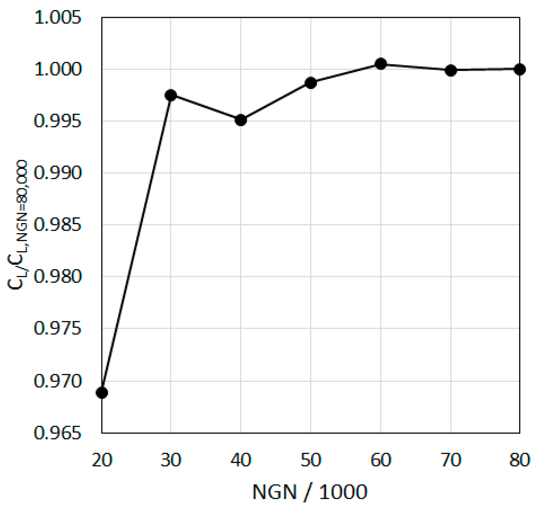
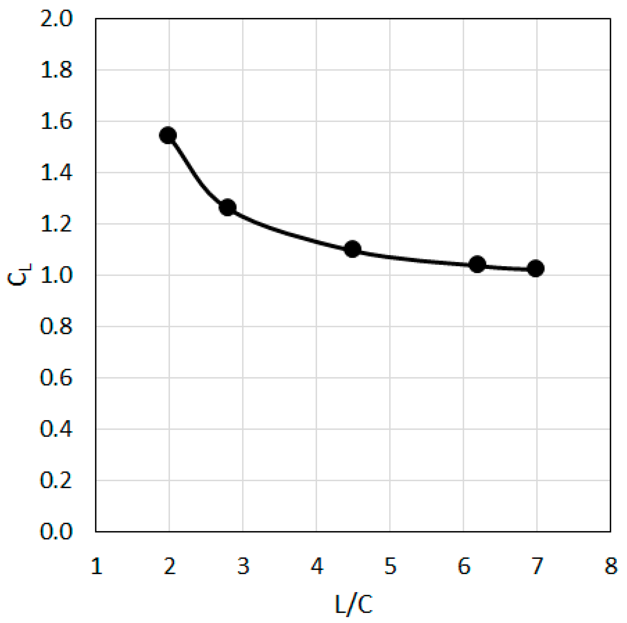
For ensuring grid independence in the CFD predictions, calculations have been performed for a typical airfoil shape and flow configuration, using different grid resolutions. The variation of the predicted lift coefficient (normalized by that of the finest grid with) with the total number of grid nodes (NGN), for the considered case is displayed in Figure 5. As it can be seen in the figure, a sufficient grid independence is achieved for grids with larger than 50,000 nodes. Following these findings, the grids are generated by the developed automatic grid generator, using the same grid topology and strategy, with an even finer resolution corresponding to number of nodes about 60,000, for assuring sufficient grid independence.

3.2. Validation

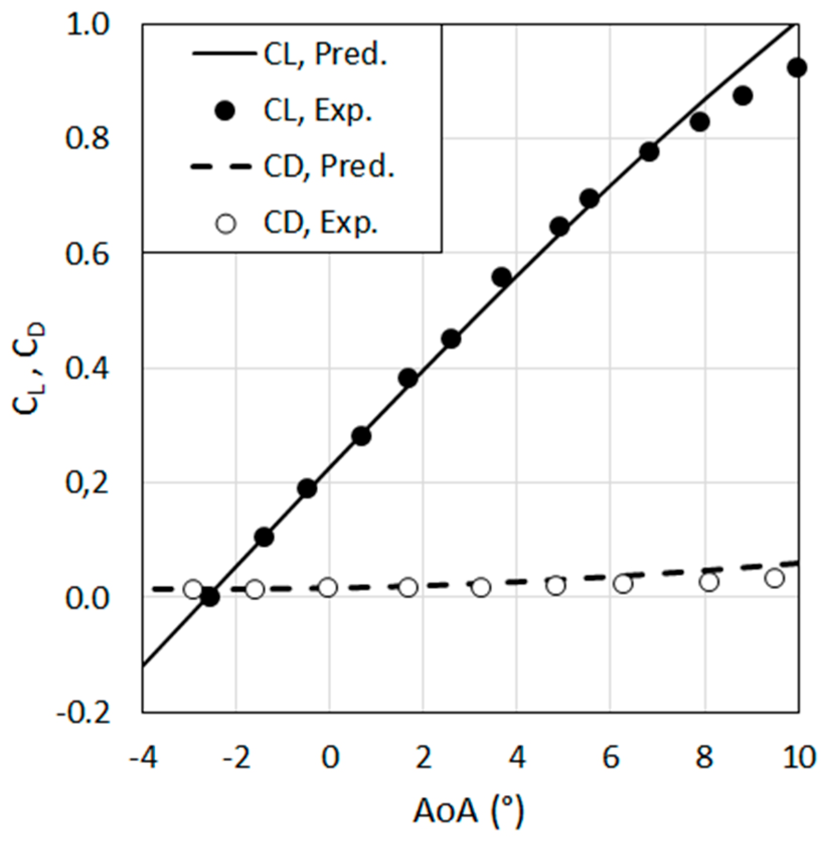
For the validation of the applied CFD methodology, the flow over the airfoil NREL-S822 of Selig et al. [51] was calculated for Re = 400,000. The predicted lift and drag coefficients as function of AoA are compared with the measured values [51] in Figure 6. A quite well overall agreement between the predictions and measurements can be observed (Figure 6).

3.3. Influence of the Domain Size, Blade to Blade Interaction

The flow around the NREL-S822 airfoil [51] is calculated for Re = 400,000, for BA = 5° and FA = 15° (AoA = 10°) for different circumferential domain sizes (L). The predicted lift coefficient as a function of dimensionless domain size (L/C) are shown in Figure 7.
As can be seen in Figure 7, the blade-to-blade interaction is negligible for L/C > 6 but becomes noticeable for lower values. The observed increasing trend of CL with decreasing L/C is the reverse of what is implied by the classical, one-dimensional linear cascade theory, which predicts a decreasing CL with decreasing L/C. This is because that the mentioned theory assumes a perfect flow deflection (which is reasonable for turbomachinery of gas and steam turbines with rather small L/C values), whereas in the present case with relatively large L/C values and, thus, non-ideal flow deflection on the average, a decrease of L/C improves the deflection of the passage flow, leading to an increase in CL.

3.4. Optimization

The parametrization of the airfoil shape was discussed in Section 2.5 and depicted in Figure 4. In the present application of the optimization algorithm, some constraints are imposed on the shape parameters, to reduce the degrees of freedom and thus the computational effort and for improving the computational stability as well as considering issues related to structural aspects and manufacturing: The two points defining the trailing edge (P1, P5) and the associated vectors of the related Hermite curves (HC1, HC4) are fixed. The lengths of the vectors that are connected to P2, P4 and head towards the trailing edge (l21, l44) are additionally assumed to be constant. The point defining the leading edge (P3) is also fixed in its position (Figure 4). Furthermore, the control points on the suction (P2) and pressure (P4) sides (Figure 4) are not allowed to move parallel to the chord but only in the perpendicular direction. An additional constraint was that the distance between P2 and P4 should not undershoot a certain value, to provide “too thin” blades, for structural reasons. Given these constraints and the continuity of the curves, the remaining degrees of freedom that define the profile shape are nine in total, that is, the vertical positions of the points P2 and P4, the directions (α2, α3, α4) and the lengths of the vector pairs (each pair have a common direction) at the points P2, P3 and P4 (l22, l32, l33, l43). The schematic of the resulting complete optimization loop is presented in Figure 8.
For the RSM, the applied factor levels and the natural values of the variables for the OCCD arrangement of the data points are provided in Table 1. Please note that the ranges covered in Table 1 are not necessarily meant to be realistic for a practical application but merely serve to an exemplarily demonstration of the procedure.
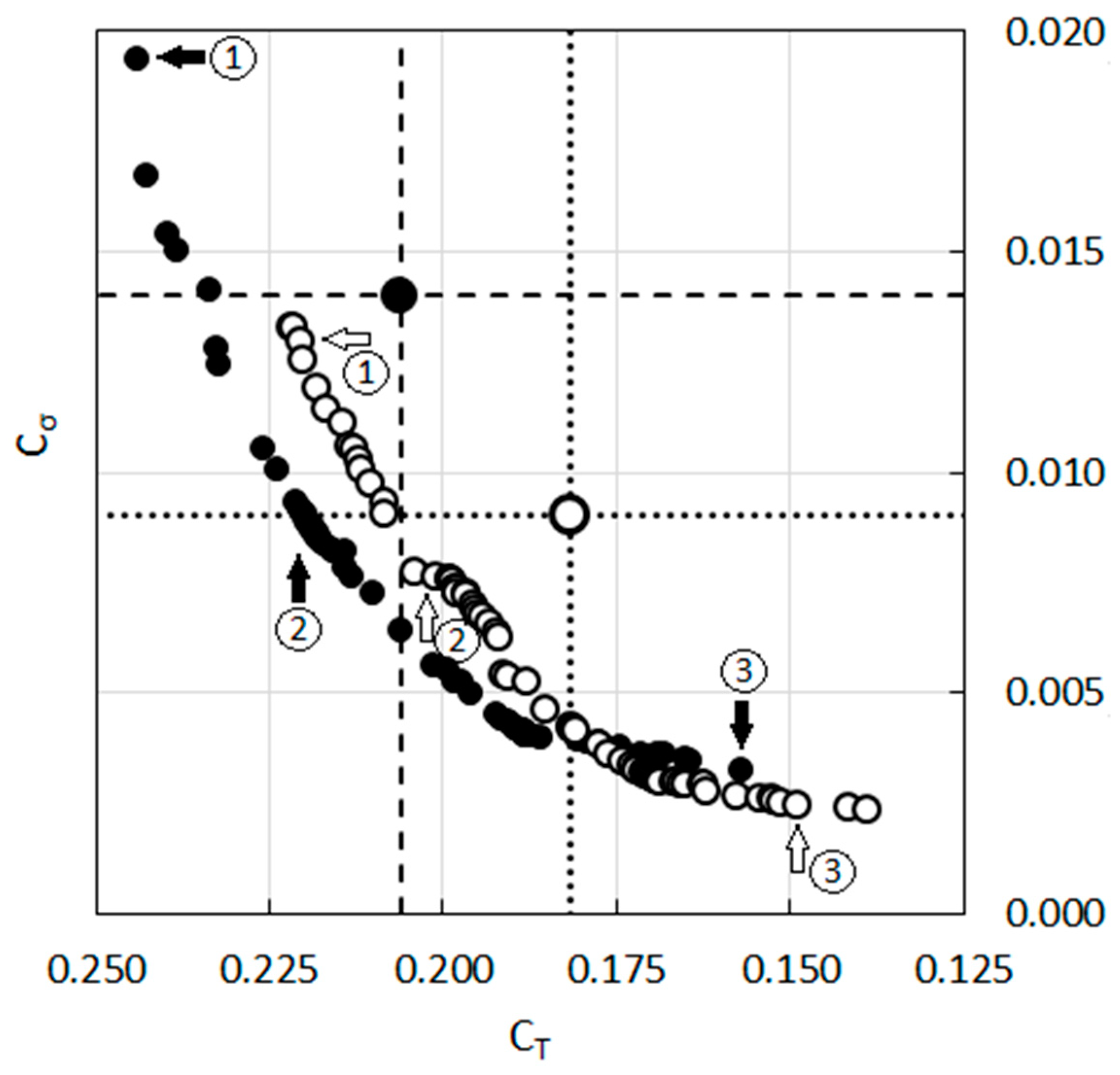
The NREL-S822 [51] is profile is taken as the basis (the original, non-optimized profile) and optimized applying the procedure described above, for the different relative domain sizes, namely for L/C = 3 and L/C = 6. Doing so, the Reynolds number (Re), which based on the approach velocity magnitude V and the chord length C, is varied by varying V, keeping C and the air properties constant. The two objective functions, that is, the high average trust (T) and low standard deviation (σ) under varying wind conditions cannot be maximized simultaneously, without making a trade-off between the two goals. The feasible choices resulting from this trade-off can be represented by the so-called Pareto front [52]. The optimization is carried out for two cases, namely for L/C = 3 and for L/C = 6, with different levels of blade-to-blade interaction. The predicted Pareto fronts for two cases, that is, for L/C = 3 and L/D = 6, are presented in Figure 9 in terms of the average thrust coefficient CT and the coefficient of thrust standard deviation Cσ that are obtained nondimensionalizing the variables by the dynamic pressure 1/2ρV2 and the chord C.
The larger circles located at the intersecting broken lines in the figure indicate the performance of the original profile before optimization. The smaller circles are the results of different optimizations, which, altogether, build-up the Pareto front. Each circle is associated with a different profile with a slightly different shape. The numbers 1, 2, 3 indicate the profiles that are exemplarily chosen for a more detailed presentation, in the following. As can be seen in the figure, the performance of the profile changes with domain size. For the same operation range (Table 1) the original profile in the small domain (L/C = 3) delivers a larger thrust on the average (large full circle in Figure 9), whereas for the large domain (L/C = 6) it performs more stable (large empty circle, Figure 9). The Pareto fronts that result from the optimization are also different for both domain sizes (Figure 9). The dashed (L/C = 3) and dotted (L/C = 6) lines that cross the larger circles (marking the original profile) define four regions, for each domain size, with different qualitative behaviour compared to the original design. All points within the lower left quadrangle represent an improvement in both objectives, whereas the points in the upper right quadrangle (if any) would mean a worsening in both. In the upper left region, the thrust is improved at the expense of a larger standard deviation (less stability of operation under varying wind conditions), whereas the reverse is true in the lower right quadrangle.
The Pareto fronts of both domain sizes are quite close to each other in the lower right part of Figure 9, implying that the airfoil shapes that are optimized for stable operation (low standard deviation, low thrust) perform similarly, irrespective of the domain size. The Pareto fronts diverge towards the upper left direction (Figure 9), implying that for the blades optimized for high thrust, the domain size plays a greater role. In this region, for the same thrust coefficient, the optimized profiles for the smaller domain (L/C = 3) seem to exhibit a better stability (lower standard deviation) compared to those of the larger domain (L/C = 6).
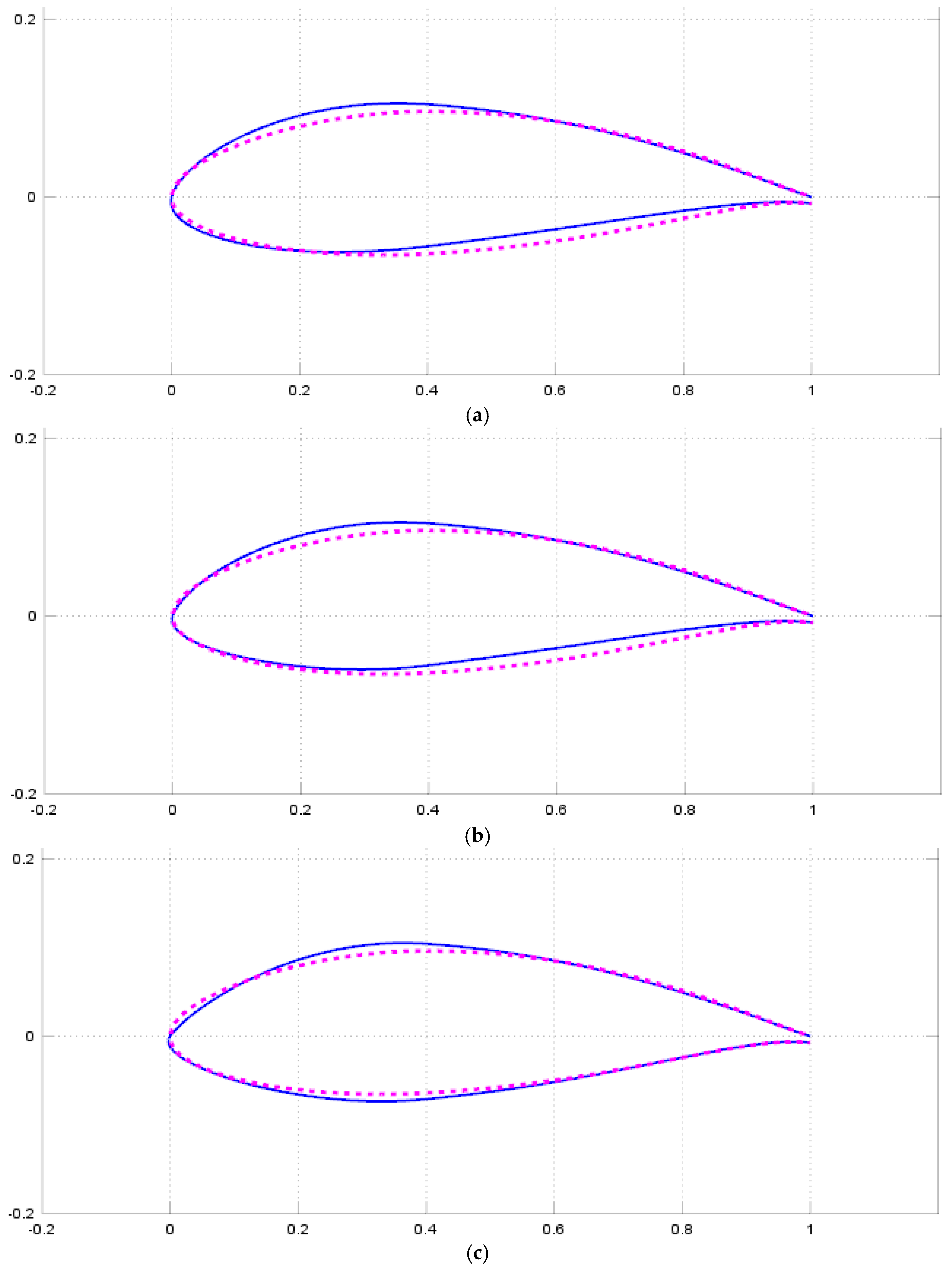
The optimized profile shapes in comparison with the original profile are presented in Figure 10 and Figure 11, for L/C = 3 and L/C = 6, respectively, for the three points indicated by arrows as 1, 2, 3 in Figure 9.
One can observe (Figure 10 and Figure 11) the differences in the optimization between the three considered points for each domain size, as well as between the two relative domain sizes. It is interesting to observe that rather small variations in the shape can have quite substantial impact on the performance.
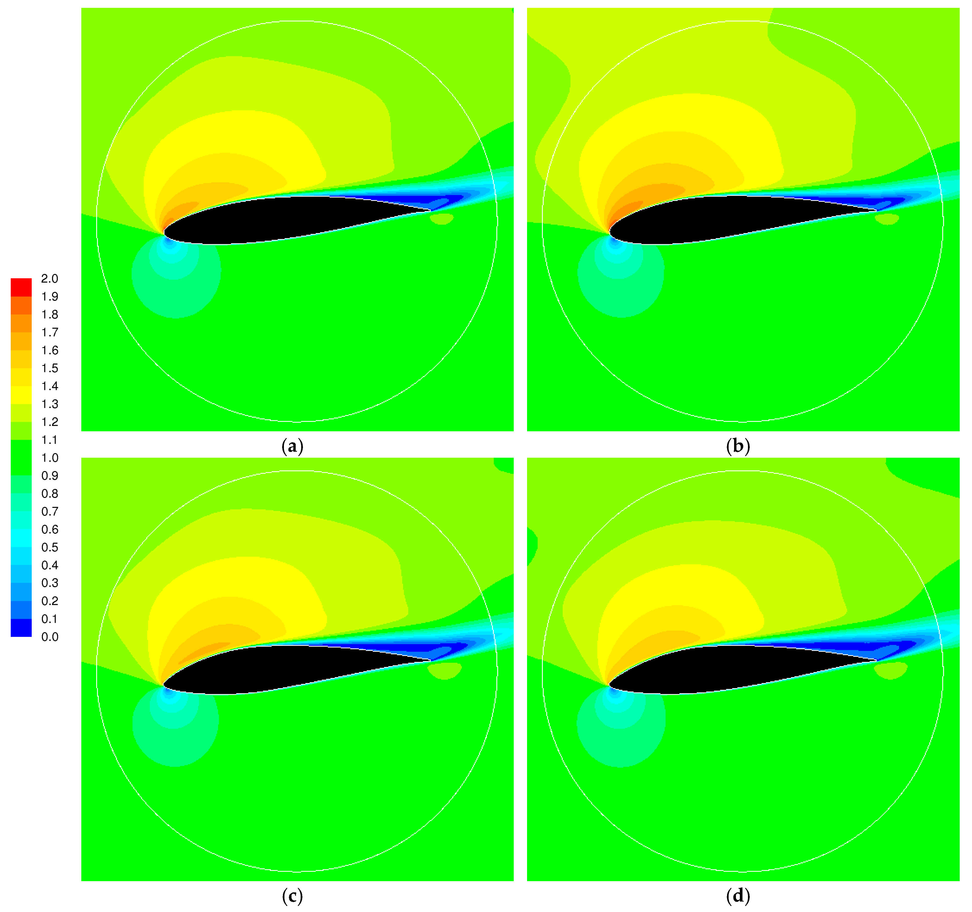
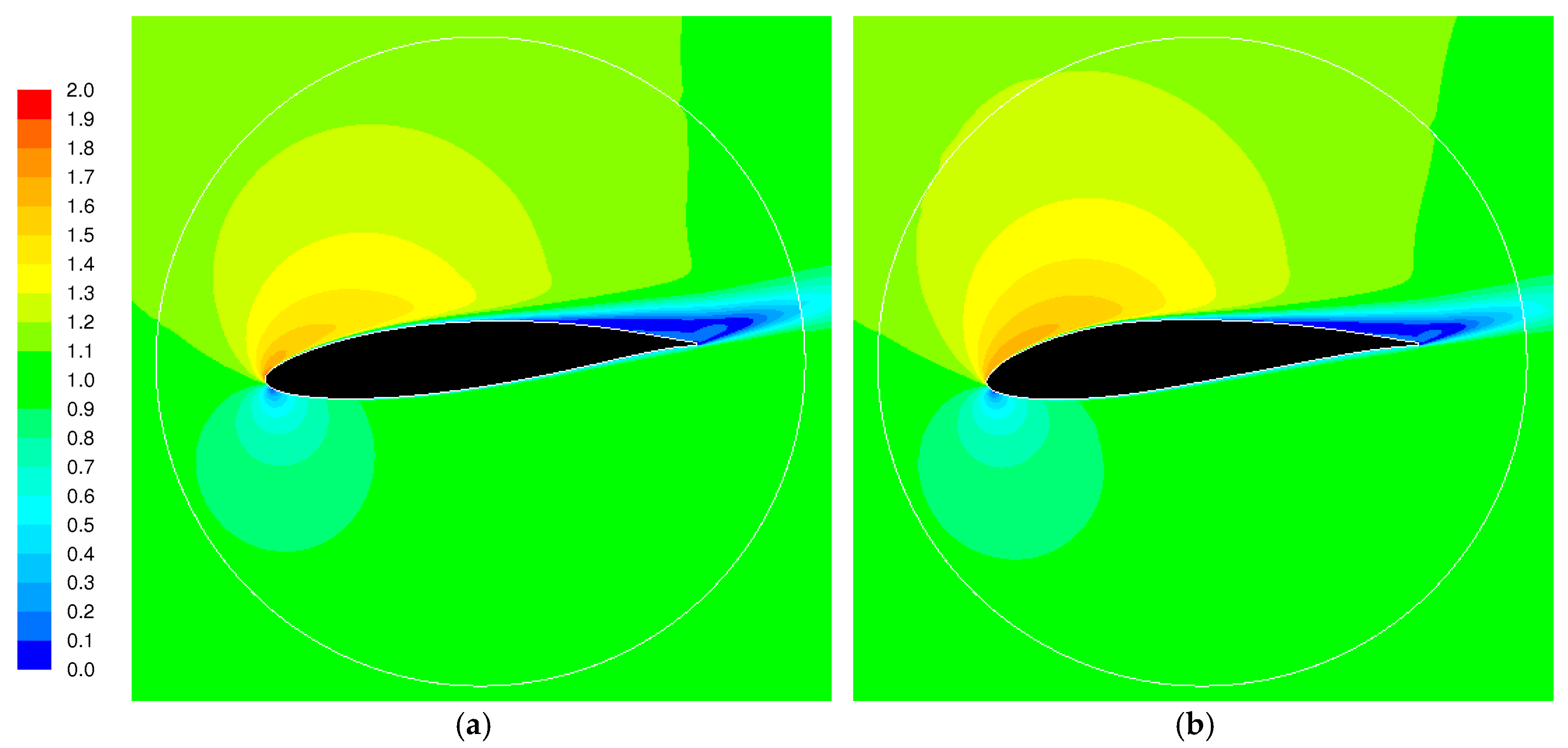
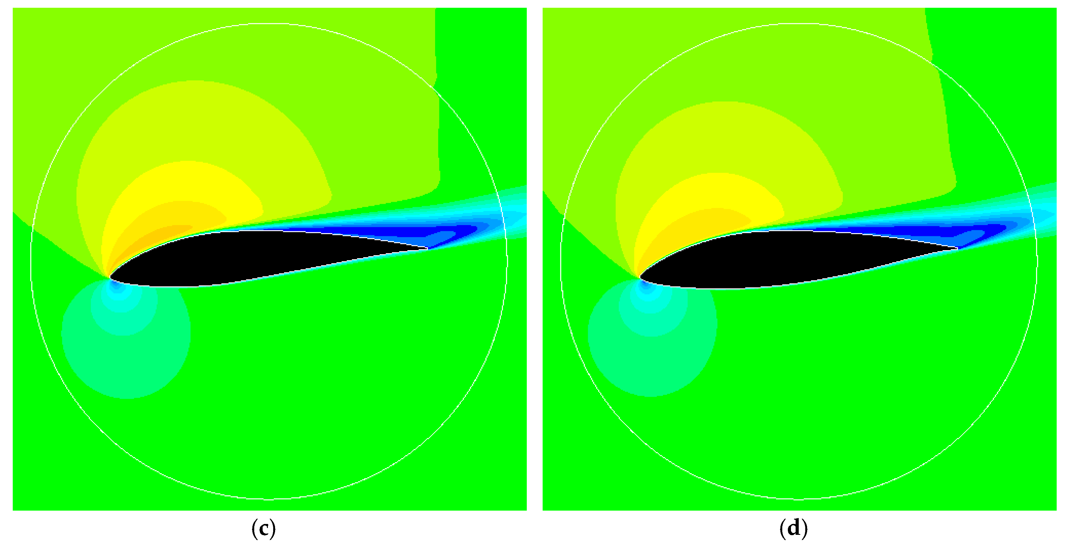
The predicted fields of non-dimensional velocity magnitude (velocity nondimensionalized by V) around the original airfoil and the three optimized airfoils corresponding to the three points (for each domain size) indicated in Figure 9 are presented in Figure 12 and Figure 13 for L/C = 3 and L/C = 6, respectively, for Re = 100,000, BA = 5°, FA = 15° (AoA = 10°).
Differences in the velocity fields with changing airfoil shape can be observed (Figure 12 and Figure 13). Note that the performances indicated in Figure 9 for different profiles are the overall (average) performances for the considered range of operation (Table 1) but are not directly connected to a given operation point. Still, the predicted velocity fields imply that the relative performance of the profiles qualitatively correspond to the trend indicated in Figure 9, where moving from Profile 1 to Profile 2 and to Profile 3 a decreasing acceleration on the suction side can be observed, implying a decreasing trend for the lift, that is, thrust, agreeing qualitatively with the behaviour shown in Figure 9.

4. Conclusions

An automated two-dimensional airfoil shape optimization procedure for small horizontal axis wind turbines (HAWT) is presented, with emphasis on high thrust and aerodynamically stable performance. The procedure combines the Computational Fluid Dynamics (CFD) analysis with the Response Surface Methodology (RSM), the Biobjective Mesh Adaptive Direct Search (BiMADS) optimization algorithm and an automatic geometry and mesh generation tool. In the CFD analysis, a Reynolds Averaged Numerical Simulation (RANS) is applied in combination with a two-equation turbulence model. In the analysis, an emphasis is placed upon the role of the blade-to-blade interaction. The results show that improvements in the performance can be achieved by modifications of the blade shape, resulting in a Pareto front and the present procedure can be used as a tool for blade shape optimization. Prioritization of the properties while choosing a profile out of the Pareto front would depend on the purpose of the application. Profiles with high thrust may, for example, be preferred for a local, direct consumption of the generated electric power, while more stably operating profiles (with low standard deviation of thrust) may be preferred for feeding the power into the grid.

Author Contributions

All the authors contributed equally to this paper.

Acknowledgments

Stefan Rohr of RLE International GmbH, Cologne, Germany is gratefully acknowledged for valuable technical discussions.

Conflicts of Interest

The authors declare no conflict of interest.

Nomenclature

Cchord length
CDdrag coefficient
CLlift coefficient
CTaverage thrust coefficient
Cσcoefficient of thrust standard deviation
Lcircumferential domain size (distance between periodic boundaries)
ReReynolds number
Tthrust
Vmagnitude of approach velocity at Re = 100,000
y+distance to wall non-dimensionalized by wall shear stress, viscosity and density
Greek symbols
ρdensity
σstandard deviation of thrust
Abbreviations
AoAAngle of Attack
BABlade Angle
BiMADSBiobjective Mesh Adaptive Direct Search
BEMBlade Element Momentum
CFDComputational Fluid Dynamics
FAFlow Angle
FVMFinite Volume Method
GAGenetic Algorithms
HAWTHorizontal Axis Wind Turbines
LESLarge Eddy Simulations
NGNNumber of Grid Nodes
OCCDOrthogonal Central Composite Design
RANSReynolds Averaged Numerical Simulations
RSMResponse Surface Methodology
SSTShear Stress Transport

References

  1. Hau, E. Wind Turbines; Springer: Berlin, Germany, 2013. [Google Scholar]
  2. Oyama, A.; Liou, M.-S.; Obayashi, S. Transonic axial-flow blade shape optimization using evolutionary algorithm and three-dimensional Navier-Stokes solver. In Proceedings of the 9th AIAA/ISSMO Symposium on Multidisciplinary Analysis and Optimization (AIAA 2002-5642), Atlanta, GA, USA, 4–6 September 2002. [Google Scholar]
  3. Semenova, A.; Chrikov, D.; Lyutiv, A.; Cherny, S.; Skorospelov, V.; Pylev, I. Multi-objective shape optimization of runner blade for Kaplan turbine. IOP Conf. Ser. Earth Environ. Sci. 2014, 22, 012025. [Google Scholar] [CrossRef]
  4. Thumthae, C.; Chitsomboon, T. Optimal angle of attack for untwisted blade wind turbine. Renew. Energy 2009, 34, 1279–1284. [Google Scholar] [CrossRef]
  5. Jureczko, M.; Pawlak, M.; Mezyk, A. Optimisation of wind turbine blades. J. Mater. Process. Technol. 2005, 167, 463–471. [Google Scholar] [CrossRef]
  6. Mendez, J.; Greiner, D. Wind blade chord and twist angle optimization by using genetic algorithms. In Proceedings of the 5th Conference on Engineering Computational Technology, Las Palmas de Gran Canaria, Spain, 12–15 September 2006. [Google Scholar]
  7. Burger, C.; Hartfield, R. Wind turbine airfoil performance optimization using the vortex lattice method and a genetic algorithm. In Proceedings of the 4th AIAA Energy Conversion Conference, San Diego, CA, USA, 26–29 June 2006. [Google Scholar]
  8. Clifton-Smith, M.; Wood, D. Further dual purpose evolutionary optimization of small wind turbine blades. J. Phys. Conf. Ser. 2007, 75, 012017. [Google Scholar] [CrossRef]
  9. Liu, X.; Chen, Y.; Ye, Z. Optimization model for rotor blades of horizontal axis wind turbines. Front. Mech. Eng. China 2007, 2, 483–488. [Google Scholar] [CrossRef]
  10. XFOIL Subsonic Airfoil Development System. Available online: http://web.mit.edu/drela/Public/web/xfoil/ (accessed on 12 April 2018).
  11. Kenway, G.; Martins, J.R.R.A. Aerostructural shape optimization of wind turbine blades considering site-specific winds. In Proceedings of the AIAA/ISSMO Multidisciplinary Analysis and Optimization Conference, Victoria, BC, Canada, 10–12 September 2008. [Google Scholar]
  12. Xudong, W.; Shen, W.Z.; Zhu, W.J.; Sorensen, J.N.; Jin, C. Shape optimization of wind turbine blades. Wind Energy 2009, 12, 781–803. [Google Scholar] [CrossRef]
  13. Ceyhan, O.; Sezer-Uzol, N.; Tuncer, I. Optimization of horizontal axis wind turbines by using BEM theory and genetic algorithm. In Proceedings of the 5th Ankara International Aerospace Conference, METU, Ankara, Turkey, 17–19 August 2009; pp. 17–19. [Google Scholar]
  14. Li, J.Y.; Li, R.; Gao, Y.; Huang, J. Aerodynamic optimization of wind turbine airfoils using response surface techniques. Proc. Inst. Mech. Eng. Part A J. Power Energy 2010, 224, 827–838. [Google Scholar] [CrossRef]
  15. Grujicic, M.; Arakere, G.; Pandurangan, B.; Sellappan, V.; Vallejo, A.; Ozen, M. Multidisciplinary design optimization for glass-fibre epoxy-matrix composite 5 MW horizontal-axis wind-turbine blades. J. Mater. Eng. Perform. 2010, 19, 1116–1127. [Google Scholar] [CrossRef]
  16. Bottasso, C.; Campagnolo, F.; Croce, A. Computational Procedures for the Multidisciplinary Constrained Optimization of Wind Turbines; Scientific Report DIA-SR; Dipartimento di Ingegneria Aerospaziale, Politecnico di Milano: Milano, Italy, 2010. [Google Scholar]
  17. Kusiak, A.; Zheng, H.Y. Optimization of wind turbine energy and power factor with an evolutionary computation algorithm. Energy 2010, 35, 1324–1332. [Google Scholar] [CrossRef]
  18. Song, F.F.; Ni, Y.H.; Tan, Z.Q. Optimization design, modeling and dynamic analysis for composite wind turbine blade. Procedia Eng. 2011, 16, 369–375. [Google Scholar] [CrossRef]
  19. Wang, L.; Wang, T.G.; Luo, Y. Improved non-dominated sorting genetic algorithm (NSGA)-II in multi-objective optimization studies of wind turbine blades. Appl. Math. Mech. Engl. Ed. 2011, 32, 739–748. [Google Scholar] [CrossRef]
  20. Grasso, F. Hybrid optimization for wind turbine thick airfoils. In Proceedings of the 53rd AIAAJASME/ASCE/AHS/ASC Structures, Structural Dynamics and Materials Conference, Honolulu, HI, USA, 23–26 April 2012. AIAA Paper AIAA-2012. [Google Scholar]
  21. Chen, X.M.; Agarwal, R. Optimization of flatback airfoils for wind-turbine blades using a genetic algorithm. J. Aircr. 2012, 49, 622–629. [Google Scholar] [CrossRef]
  22. Ribeiro, A.F.P.; Awruch, A.M.; Gomes, H.M. An airfoil optimization technique for wind turbines. Appl. Math. Model. 2012, 36, 4898–4907. [Google Scholar] [CrossRef]
  23. Jeong, J.; Park, K.; Jun, S.; Song, K.; Lee, D.H. Design optimization of a wind turbine blade to reduce the fluctuating unsteady aerodynamic load in turbulent wind. J. Mech. Sci. Technol. 2012, 26, 827–838. [Google Scholar] [CrossRef]
  24. Ju, Y.P.; Zhang, C.H. Multi-point robust design optimization of wind turbine airfoil under geometric uncertainty. Proc. Inst. Mech. Eng. Part A J. Power Energy 2012, 226, 245–261. [Google Scholar] [CrossRef]
  25. Liao, C.C.; Zhao, X.L.; Xu, J.Z. Blade layers optimization of wind turbines using FAST and improved PSO algorithm. Renew. Energy 2012, 42, 227–233. [Google Scholar] [CrossRef]
  26. Polat, O.; Tuncer, I.H. Aerodynamic shape optimization of wind turbine blades using a parallel genetic algorithm. Procedia Eng. 2013, 61, 28–31. [Google Scholar] [CrossRef]
  27. Sessarego, M.; Dixon, K.R.; Rival, D.E.; Wood, D.H. A hybrid multi-objective evolutionary algorithm for wind-turbine blade optimization. Eng. Optim. 2015, 47, 1043–1062. [Google Scholar] [CrossRef]
  28. Shen, X.; Chen, J.E.; Zhu, X.C.; Liu, P.Y.; Du, Z.H. Multi-objective optimization of wind turbine blades using lifting surface method. Energy 2015, 90, 1111–1121. [Google Scholar] [CrossRef]
  29. Hassanzadeh, A.; Hassanabad, A.H.; Dadvand, A. Aerodynamic shape optimization and analysis of small wind turbine blades employing the Viterna approach for post-stall region. Alex. Eng. J. 2016, 55, 2035–2043. [Google Scholar] [CrossRef]
  30. Pourrajabian, A.; Afshar, P.A.N.; Ahmadizadeh, M.; Wood, D. Aero-structural design optimization of a small wind turbine blade. Renew. Energy 2016, 87, 837–848. [Google Scholar] [CrossRef]
  31. Dal Monte, A.; De Betta, S.; Castelli, M.R.; Benini, E. Proposal for a coupled aerodynamic-structural wind turbine blade optimization. Compos. Struct. 2017, 159, 144–156. [Google Scholar] [CrossRef]
  32. Chehouri, A.; Younes, R.; Ilinca, A.; Perron, J. Review of performance optimization applied to wind turbines. Appl. Energy 2015, 142, 361–388. [Google Scholar] [CrossRef]
  33. Myers, R.H.; Montgomery, D.C.; Anderson-Cook, C.M. Response Surface Methodology: Process and Product Optimization Using Designed Experiments, 4th ed.; Wiley: Hoboken, NJ, USA, 2016. [Google Scholar]
  34. Benim, A.C.; Brillert, D.; Cagan, M. Investigation into the computational analysis of direct-transfer pre-swirl systems for gas turbine cooling. In Proceedings of the ASME Turbo Expo 2004, Vienna, Austria, 14–17 June 2004; Volume 4, pp. 453–460, Paper No. GT2004-54151. [Google Scholar] [CrossRef]
  35. Benim, A.C.; Geiger, M.; Doehler, S.; Schoenenberger, M.; Roemer, H. Modelling the Flow in the Exhaust Hood of Steam Turbines under Consideration of Turbine-Exhaust Hood Interaction. In Proceedings of the 1st European Conference on Turbomachinery—Fluid Dynamic and Thermodynamic Aspects: Computational Methods, Erlangen, Germany, 1–3 March 1995; Book Series: VDI Berichte; VDI Verlag: Duesseldorf, Germany, 1995; Volume 1185, pp. 343–357. [Google Scholar]
  36. Engineering Simulations and 3-D Design Software. Available online: www.ansys.com (accessed on 17 October 2018).
  37. Durbin, P.A.; Pettersson Reif, B.A. Statistical Theory and Modeling for Turbulent Flows, 2nd ed.; Wiley: Chichester, UK, 2011. [Google Scholar]
  38. Benim, A.C.; Nahavandi, A.; Syed, K. URANS and LES analysis of turbulent swirling flows. Prog. Comput. Fluid Dyn. An Int. J. 2005, 5, 444–454. [Google Scholar] [CrossRef]
  39. Benim, A.C.; Chattopadhyay, H.; Nahavandi, A. Computational analysis of turbulent forced convection in a channel with a triangular prism. Int. J. Therm. Sci. 2011, 50, 1973–1983. [Google Scholar] [CrossRef]
  40. Menter, F.; Esch, T.; Kubacki, S. Transition modelling based on local variables. In Proceedings of the Fifth International Symposium on Engineering Turbulence Modelling and Measurements, Mallorca, Spain, 16–18 September 2002; Engineering Turbulence Modelling and Experiments 5. Rodi, W., Fueye, N., Eds.; Elsevier: Amsterdam, The Netherlands, 2002; pp. 555–564. [Google Scholar]
  41. Benim, A.C.; Cagan, M.; Gunes, D. Computational analysis of transient heat transfer in turbulent pipe flow. Int. J. Therm. Sci. 2004, 43, 725–732. [Google Scholar] [CrossRef]
  42. Benim, A.C.; Ozkan, K.; Cagan, M.; Gunes, D. Computational investigation of turbulent jet impinging onto rotating disk. Int. J. Numer. Methods Heat Fluid Flow 2007, 17, 284–301. [Google Scholar] [CrossRef]
  43. Assmann, A.; Benim, A.C.; Gül, F.; Lux, P.; Akhyari, P.; Boeken, U.; Joos, F.; Feindt, P.; Lichtenberg, A. Pulsatile extracorporeal circulation during on-pump cardiac surgery enhances aortic wall shear stress. J. Biomech. 2012, 45, 156–163. [Google Scholar] [CrossRef] [PubMed]
  44. Deng, G.B.; Ferry, M.; Piquet, J.; Queutey, P.; Visonneau, M. New fully coupled solutions of the Navier-Stokes equations. In Notes on Numerical Fluid Mechanics (NNFM), Proceedings of the 9th GAMM Conference on Numerical Methods in Fluid Mechanics, Lausanne, Switzerland, 25–27 September 1991; Vos, J.B., Ed.; Springer: Wiesbaden, Germany, 1992; Volume 35, pp. 191–200. [Google Scholar]
  45. Leonard, B.P. A stable and accurate convective modelling procedure based on quadratic upstream interpolation. Comput. Methods Appl. Mech. Eng. 1979, 19, 59–98. [Google Scholar] [CrossRef]
  46. Barth, T.J.; Jespersen, D. The design and application of upwind schemes on unstructured meshes. In Proceedings of the AIAA 27th Aerospace Sciences Meeting, Reno, NV, USA, 9–12 January 1989. Technical Report AIAA-89-0366. [Google Scholar]
  47. Benim, A.C.; Pasqualotto, E.; Suh, S.H. Modeling turbulent flow past a circular cylinder by RANS, URANS, LES and DES. Prog. Computat. Fluid Dyn. An Int. J. 2008, 8, 299–307. [Google Scholar] [CrossRef]
  48. GNU Octave. Available online: https://www.gnu.org/software/octave/ (accessed on 17 April 2018).
  49. Conn, A.R.; Scheinberg, K.; Vincente, L.N. Introduction to Derivative-Free Optimization; SIAM: Philadelphia, PA, USA, 2009. [Google Scholar]
  50. Le Digabel, S. Algorithm 909: NOMAD: Nonlinear Optimization with the MADS Algorithm. ACM Trans. Math. Softw. 2011, 37, 44. [Google Scholar] [CrossRef]
  51. Selig, M.S.; Lyon, C.A.; Giguère, P.; Ninham, C.P.; Guglielmo, J.J. Summary of Low-Speed Airfoil Data; Soar Tech Publications: Virginia Beach, VA, USA, 1996; Volume 2. [Google Scholar]
  52. Branke, J.; Deb, K.; Miettinen, K.; Slowinski, R. (Eds.) Multiobjective Optimization; Springer: Berlin, Germany, 2008. [Google Scholar]
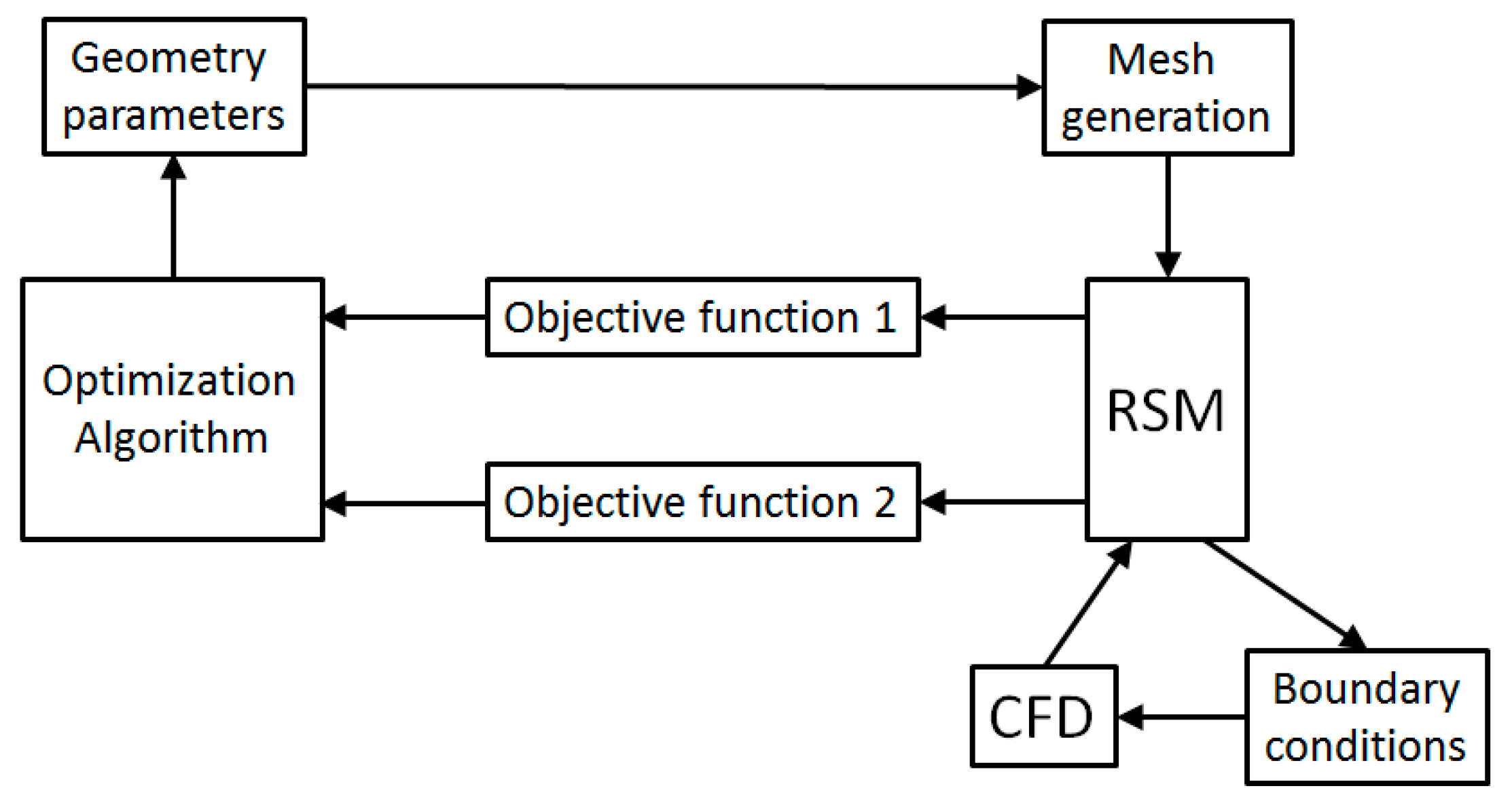
Figure 1. Optimization cycle.
Computation 06 00034 g001
Figure 2. Solution domain and boundaries.
Computation 06 00034 g002
Figure 3. Detail view of a typical grid.
Computation 06 00034 g003
Figure 4. Parametric representation of airfoil shape by Hermite curves.
Computation 06 00034 g004
Figure 5. Variation of predicted lift coefficient with grid resolution.
Computation 06 00034 g005
Figure 6. Comparison of predicted lift and drag coefficients with the measured values for the profile NREL-S822 of Selig et al. [51] (Re = 400,000).
Computation 06 00034 g006
Figure 7. Variation of the predicted lift coefficient with circumferential domain size, for Re = 400,000, BA = 5°, FA = 15° (AoA = 10°).
Computation 06 00034 g007
Figure 8. Detailed representation of the optimization cycle.
Computation 06 00034 g008
Figure 9. Predicted Pareto fronts of feasible solutions of optimization. Full circles: L/C = 3, Empty circles: L/C = 6.
Computation 06 00034 g009
Figure 10. Optimized airfoil shapes for L/C = 3, for the points indicated by full arrows in Figure 9 (a) Point 1; (b) Point 2; (c) Point 3 (Figure 8), red dotted line: original, blue solid line: optimized (note that vertical scale is larger than horizontal scale).
Computation 06 00034 g010
Figure 11. Optimized airfoil shapes for L/C = 6, for the points indicated by empty arrows in Figure 9 (a) Point 1; (b) Point 2; (c) Point 3 (Figure 8), red dotted line: original, blue solid line: optimized (note that vertical scale is larger than horizontal scale).
Computation 06 00034 g011
Figure 12. Predicted distribution of dimensionless velocity magnitude around the airfoil for Re = 100,000, BA = 5°, FA = 15° (AoA = 10°), for L/C = 3, (a) Original profile; (b) Point 1; (c) Point 2; (d) Point 3 (Figure 9).
Computation 06 00034 g012
Figure 13. Predicted distribution of dimensionless velocity magnitude around the airfoil for Re = 100,000, BA = 5°, FA = 15° (AoA = 10°), for L/C = 6, (a) Original profile; (b) Point 1; (c) Point 2; (d) Point 3 (Figure 9).
Computation 06 00034 g013aComputation 06 00034 g013b
Table 1. Factor levels and the natural values of the variables (BA = 5°).
Normalized Scale Parameters
Variable−1.414−1011.414
Re/1039092.93100107.07110
FA (°)1011.461518.5420