Abstract
In this work, we study the influence of hidden barriers on the convergence behavior of three free-energy calculation methods: well-tempered metadynamics (WTMD), adaptive-biasing forces (ABF), and on-the-fly parameterization (OTFP). We construct a simple two-dimensional potential-energy surfaces (PES) that allows for an exact analytical result for the free-energy in any one-dimensional order parameter. Then we chose different CV definitions and PES parameters to create three different systems with increasing sampling challenges. We find that all three methods are not greatly affected by the hidden-barriers in the simplest case considered. The adaptive sampling methods show faster sampling while the auxiliary high-friction requirement of OTFP makes it slower for this case. However, a slight change in the CV definition has a strong impact in the ABF and WTMD performance, illustrating the importance of choosing suitable collective variables.
1. Introduction
The basic operation of a molecular dynamics (MD) simulation is numerical integration of equations of motion of a set of interacting atoms to generate discrete trajectories of atomic positions and velocities (“configuration”). Time-averaging properties of configuration from such trajectories is ideally identical to ensemble-averaging at equilibrium [1], provided the ergodic hypothesis holds at finite times. Unfortunately, most MD trajectories are not ergodic, leaving sometimes important regions of configuration space unexplored. This lack of ergodicity formally results from the fact that we cannot run infinitely long MD simulations, but it practically results from the fact that high-probability regions of configuration space are often separated by regions of low probability.
Methods of “ergodicitizing” MD simulations have a long history [2], and include “collective-variable biasing” methods such as umbrella sampling [3], thermodynamic integration [4], and much more, as well as “tempering” approaches such as simulated annealing [5] and replica-exchange [6,7]. Because these methods and their rapidly growing set of descendants all aim in one way or another to generate the correct equilibrium statistics of one or more variables of interest, they are often referred to generically as “free-energy” calculations. However, relative to the number of methodological developments in free-energy calculations, detailed comparative analysis of these methods remains underrepresented.
Collective-variable approaches are judged by how computationally efficiently they can produce an accurate free-energy as a function of the collective variable. This efficiency is most sensitively determined by how well they can handle naturally occurring restrictions to sampling in the unbiased coordinates, or so-called “hidden” barriers. Strictly speaking, unbiased coordinates must be ergodically sampled in order for the statistics along the CV to be accurate, but how close to this condition we must come for a tolerable level of accuracy, for a given choice of CV, and for a given method are not always clear.
To make matters worse, the very fact that these sampling restrictions cause inaccuracies is often difficult if not impossible to detect in production all-atom simulations. As an example, we recently showed in a study of the prion protein conformational thermodynamics that the popular CV-biasing approach Well-Tempered Metadynamics (WTMD) [8,9] can suffer a severe pathology in computing a one-dimensional free-energy profile that evidently stems from the method’s history-dependent bias [10]. We presented an approach for calculating the same FEP using enhanced sampling without a history-dependent bias, termed “on-the-fly parameterization” (OTFP) [11] that showed better convergence properties than did WTMD.
Spurred by this previous work, we take the opportunity here to investigate the convergence behavior of the history-dependent biasing approaches of WTMD and adaptive-biasing forces (ABF) [12], and the history-independent approach OTFP, in very simple, analytically tractable low-dimensional systems. Our aim is to partially elucidate properties of configuration space that most likely lead to pathologies, or at least compromised convergence, in these methods in systems where we have full a priori knowledge of all sampling restrictions.
2. Methods
We have run WTMD [8], ABF [12] and OTFP [11] methods to recover a 1D free-energy profile (FEP) from a simple 2D potential energy surface (PES). We use NAMD 2.12 [13], and the native ABF [12,14] and WTMD [8] implementations therein, and refer interested readers to those publications for detailed quantitative descriptions of those methods. The OTFP method used here is exactly that detailed in our previous work [11]. We recognize that these methods are under continuous improvement (see, e.g., [9,15,16]), but here we intend to understand fundamental differences among these approaches.
For the one-dimensional case, the FEP is defined as (up to a constant):
where is the Boltzmann constant, T the temperature and ⟨⟩ means the average over the equilibrium distribution of configuration. The Dirac delta collects those configurations of the ensemble that yield the CV’s equal to z. ABF reconstructs this by an algorithm that converges upon the mean forces, , by applying a scaled, accumulated negative estimate of those forces. WTMD reconstructs the FEP by adaptively converging to an energy bias (rather than a force bias) that can be processed to provide the FEP. OTFP uses temperature-accelerated MD (TAMD) [17] to enhance sampling along a CV, and accumulates mean-force estimates on-the-fly that can at any point be used to parameterize an analytical expansion of the free energy via gradient optimization [11].
The goal of the present work is to study the impact of “hidden barriers” on the convergence behavior of different free-energy methods. In order to do that we construct a simple model described by the following PES:
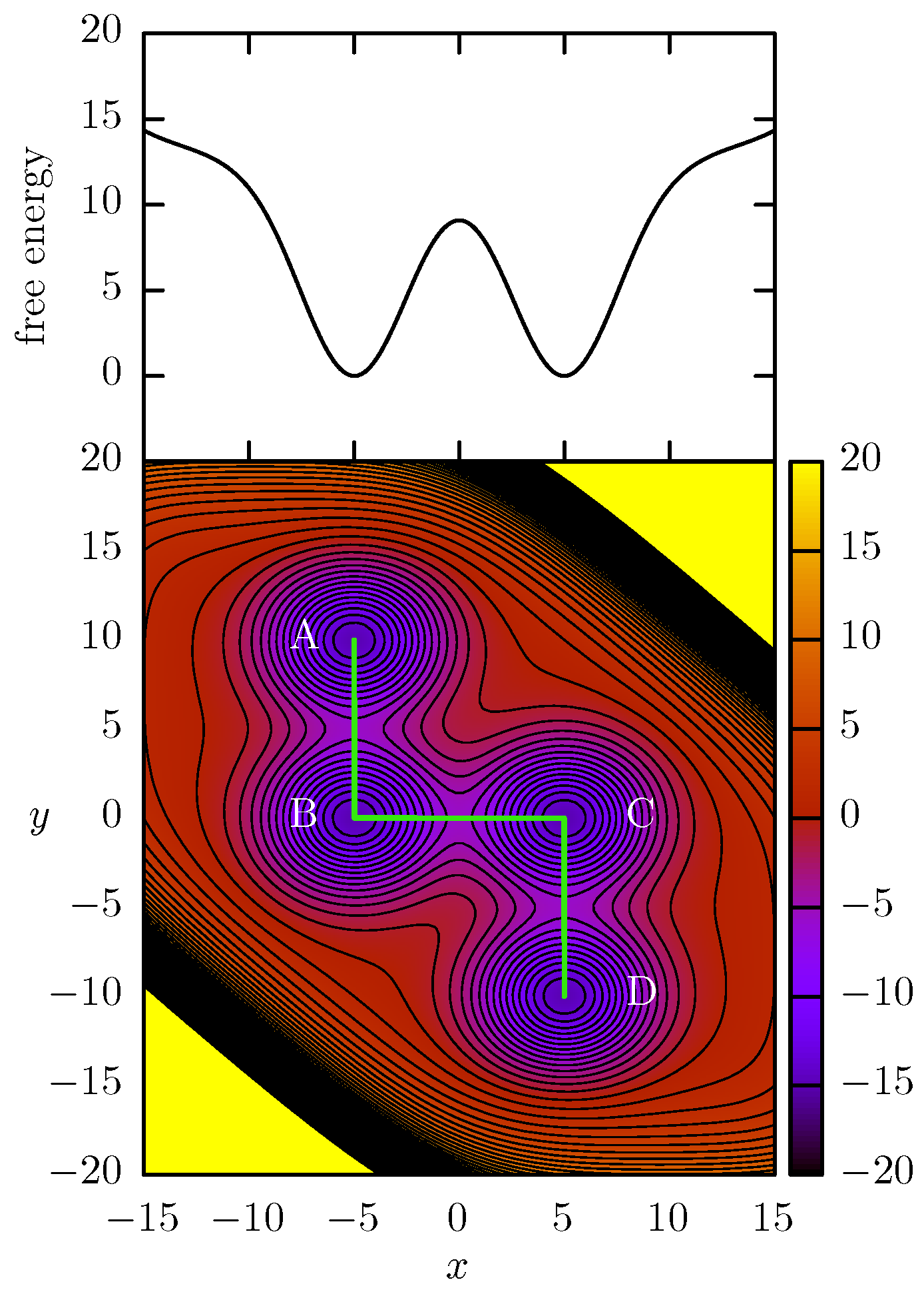
The gaussian terms generates the different basins in the PES and the last three terms serves as a boundary to confine the system dynamics around them. In particular, we used , and , with the center of the gaussian functions at , , and . With this parameters, the PES basins are distributed in a kink shape, as can be seen in the contour plot of Figure 1. We will use the A, B, C and D labels to refer to the corresponding minima as it is shown in the figure. With this model, we can select the x direction as the CV for the free-energy reconstruction while keeping slow “forgotten” modes along the y dimension. Thus, the use of a CV-biasing method will allow the acceleration of the transition through the energy barrier at , but the transition and will not be accelerated and their barriers at and become “hidden barriers”.
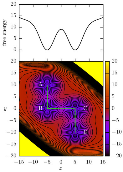
Figure 1.
Kink-shaped potential-energy sourface (k-PES) together with its free-energy profile (FEP) along the x coordinate. The minimum energy path (MEP) is shown in white on the surface and its profile is included in Figure S1 of the Supplementary Materials. The barrier height along the MEP is around 9.3.
From the point of view of ABF, WTMD or OTFP, x is a bad CV because it does not include all the slow modes of the system, a condition that must be fulfilled to achieve system acceleration and avoid sampling issues. However, as we explained in the introduction, for real-life systems it is reasonable to consider that the presence of hidden barriers will be the most general case since there are several non-accelerated dimensions (, being M the number of CVs and N the number of atoms) that could hide unknown metastable states. In our simple model, the hidden barriers generated by the existence of the A and D states can be considered the most simple case of hidden barriers since their corresponding transitions are completely orthogonal to the chosen CV. On the other hand, the metastable states A and D are aligned in x with the minima of the middle channel. Therefore, the presence of hidden barriers will occur at the same CV values of the FEP minima. The hidden barriers can occur in any region of the CV domain, and it would be of interest to study the influence of them at different positions of the middle channel. We turn to this in the second half of the results below.
For all the simulations presented in this work, the system evolves following a Langevin dynamics using a mass of , a time step of , and a coupling coefficient of . In the case of OTFP/TAMD method, the auxiliary particle evolves following a Brownian dynamics with the same time step . For OTFP it is require to assume a functional form of the free-energy to be parametrized. As in our previous works [10,11,16] we used a linear decomposition
where are the basis functions and are the coefficient of the expansion and the parameters to be adjusted by OTFP. The basis functions are constructed using simple chapeau functions (see [10,11] for more details).
3. Results
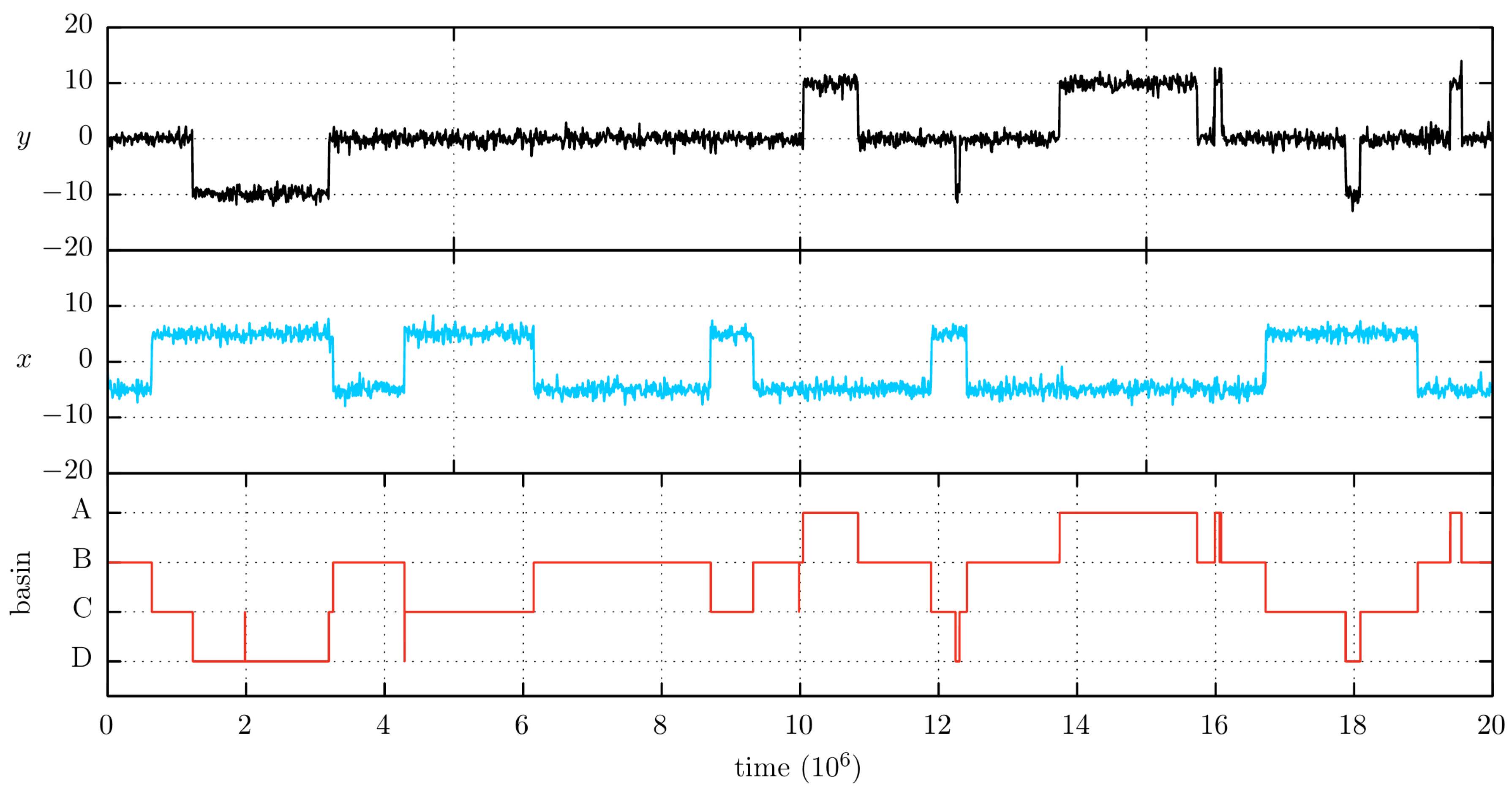
Before conducting our free-energy calculations, the first important variable to fix is the system temperature T. Since we want to accelerate the x direction we need first to emulate the behavior of a “rare-event” evolution on this dimension. Thus, we need a temperature that allows very few transition events along x during an MD simulation. At the same time, we want to operate in a regime where there is some activity along the orthogonal direction as well, even if that direction is not ergodically sampled, because hidden barriers that are never crossed by definition will not lead to problems in reproducibility of results. Thus, we need to explore the behavior of the MD simulations at different temperatures. Figure 2 shows the position traces of an MD simulation at , the temperature that was finally chosen. The traces for other temperatures can be found in Figure S2 of the Supplementary Materials. Using and x as CV, we numerically integrate Equation (1) to obtain the double-well free-energy profile (FEP) shown on top of Figure 1.
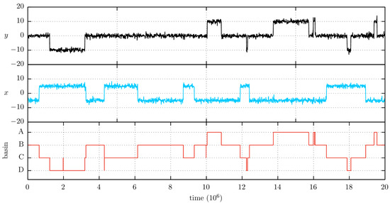
Figure 2.
MD trace for the PES show in Figure 1 at . The x and y coordinates are plot are the top (black) and middle panel (blue) respectively. The bottom panel (red) shows the basin assignation using a Voronoi tessellation for the PES minima and a running average of 5 time units as is explained in the text.
To help the reader to understand the transitions events between the various basins, we include together with the x and y traces the information of the trapping basis as a function of time (shown in red in Figure 2). To assign a trapping basin label to an instantaneous configuration we begin by associating a set of consecutive integer numbers (e.g., 4, 3, 2 and 1) to the A, B, C and D minima. Then, we perform a Voronoi tessellation from the PES minima to decide which integer number will be associated with each configuration. Finally, we perform a running average of the resulting numeric trace, in order to avoid the apparent basin changes at very short simulation times. That is, since the acceleration method increases the likelihood of observing high-energy configurations, we frequently observe a rapid backward and forward crossing across the boundaries of a tessellation cell, a feature that could be easily be confused with a change in the sampling state. Thus, we found that a running average can considerably improve the assignment of the trapping state. We have taken an interval of time units to perform this operation (note the trace has time units). The basin trace information is included any time we show a simulation trace.
Besides the system temperature, another temperature that has to be chosen is the bias sampling temperature of the WTMD and OTFP methods. In the case of WTMD this is the temperature associated with the target distribution, while in the case of OTFP, this is the temperature associated with the distribution of the auxiliary variables of TAMD. In any case, these two distributions are exactly the same:
where T is the system temperature and is called the bias temperature in the WTMD framework. While WTMD converges to this accelerated distribution at long simulation times, the OTFP/TAMD method starts sampling it from the beginning of the simulation. Given that both methods use the same accelerated distribution, we have chosen the same value in all the OTFP and WTMD simulations. Note that ABF does not have a bias temperature or an analogous parameter because at long time it converges to the uniform distribution, because the ABF force converges to the negative mean force.
Each free-energy method used in this work has its own set of parameters and some of these parameters have to be chosen carefully to ensure optimum convergence. The key parameters of WTMD are the deposition rate of the bias potential and the width of the Gaussian hills deposited. The rate is the product of the Gaussian height and the deposition frequency. We ran some test simulations to explore the convergence of WTMD for different parameter values (see Figures S3 and S4 in the Supplementary Materials). By inspecting these plots we have selected a hill deposition every 100 time steps, a Gaussian width of 1 and a height of . For the OTFP/TAMD simulations, once the auxiliary temperature is fixed, we need to choose the friction of the auxiliary particle and the spring constant between it and the configuration. The latter is easy to fix, since it is only required to be strong enough to keep the system in a small region of the CV space around the auxiliary particle. We select a spring constant of 1500, which was found to be an adequate value (see Figures S5 and S6 in the Supplementary Materials). In this way the averaged forces that the system exerts on the auxiliary particle will be a good approximation of the FEP gradient in the auxiliary particle position. The OTFP/TAMD auxiliary friction is a more important parameter in the method convergence. It has to be high enough to ensure there adiabatic decoupling of the system and the auxiliary particle dynamics. At the same time, the higher the friction is, the slower will be the sampling of the auxiliary particle across the CV space. We have chosen a friction value of 5000 times the system friction . Finally, to avoid non-equilibrium effects in ABF, we have chosen to apply the bias in each bin after the gradient as been at least measured 100 times.
The average convergence is determined by running 10 independent simulations for each system and each method and computing the resulting average FEPs for each case. These average FEPs are shown in the Figures S7–S9 of the Supplementary Materials. The average results show that the statistics of 10 independent simulations are enough to obtain a good sampling of the hidden barriers and recover the true FEP for all the cases studied in this work. The convergence to the true FEP allows us to ensure that the method parameters were properly chosen, especially parameters such as the Gaussian width in WTMD and the auxiliary friction in TAMD. If these parameters are badly chosen, the methods would have serious issues, such as convergence to an incorrect FEP. Finally, we show here the results of each individual simulation, since it is from the individual simulations where the statistics are not enough to achieve a good sampling of the hidden barrier that we can study its harmful effects, which is the goal of the paper.
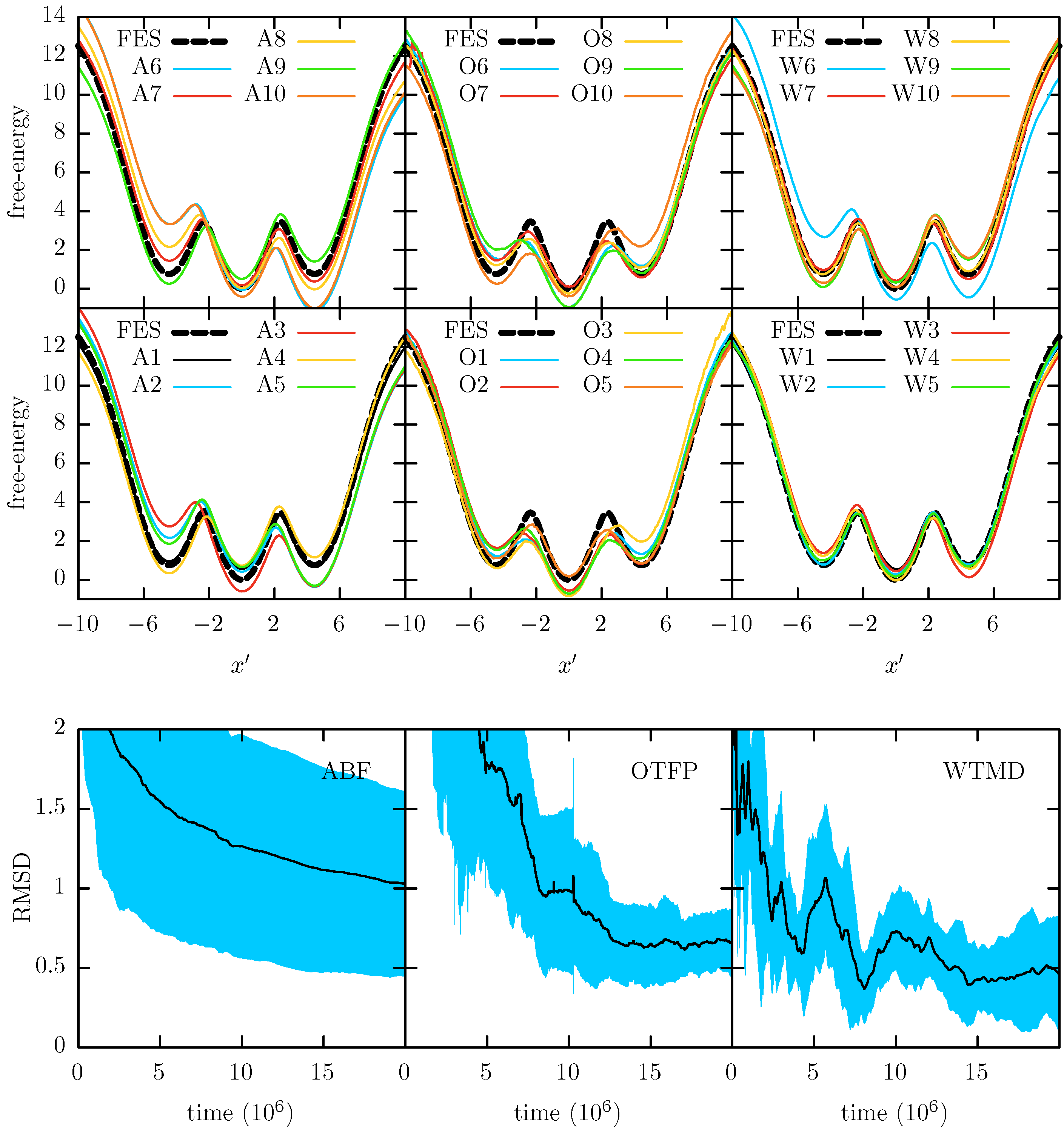
In Figure 3 we show each of the 10 independent FEPs reconstructed via ABF, WTMD and OTFP along the x CV together with the “true” FEP computed via a direct (numerical) integration of Equation (1). The reconstructed and the true FEPs are mutually aligned via least squares. In the same figure we also show the average convergence profiles for each method with its standard deviation. Note that these profiles result from averaging the individual convergence profiles, so each represents the expected convergence behavior of one individual simulation. These individual convergence profiles are obtained by measuring the root mean square deviation (RMSD) between the reconstructed profiles and the true FEP at each time, after their alignment via least square. In Figure 3 it is possible to see that the three methods give an accurate approximation of the FEP and all of them reach a good convergence below an RMSD of 0.5 after a simulation time of 20 steps. However, it is notable that ABF and WTMD obtain a better convergence than OTFP.
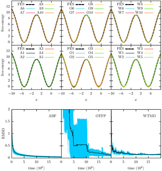
Figure 3.
FEPs obtained using x as CV and 10 different simulations for each free energy method as indicated: A1–A10 for ABF, O1–O10 for OTFP and W1–W10 for WTMD. The dashed lines correspond to the FEP computed via a direct (numerical) integration of Equation (1). The average convergence profiles are also shown in the bottom of the figure. The light blue region corresponds to one standard deviation. This profiles shows the expected convergence of each individual simulation and should not be confused with the convergence of the average FEP profile. For the average FEP and the individual convergence profiles see Figure S7 in the Supplementary Materials.
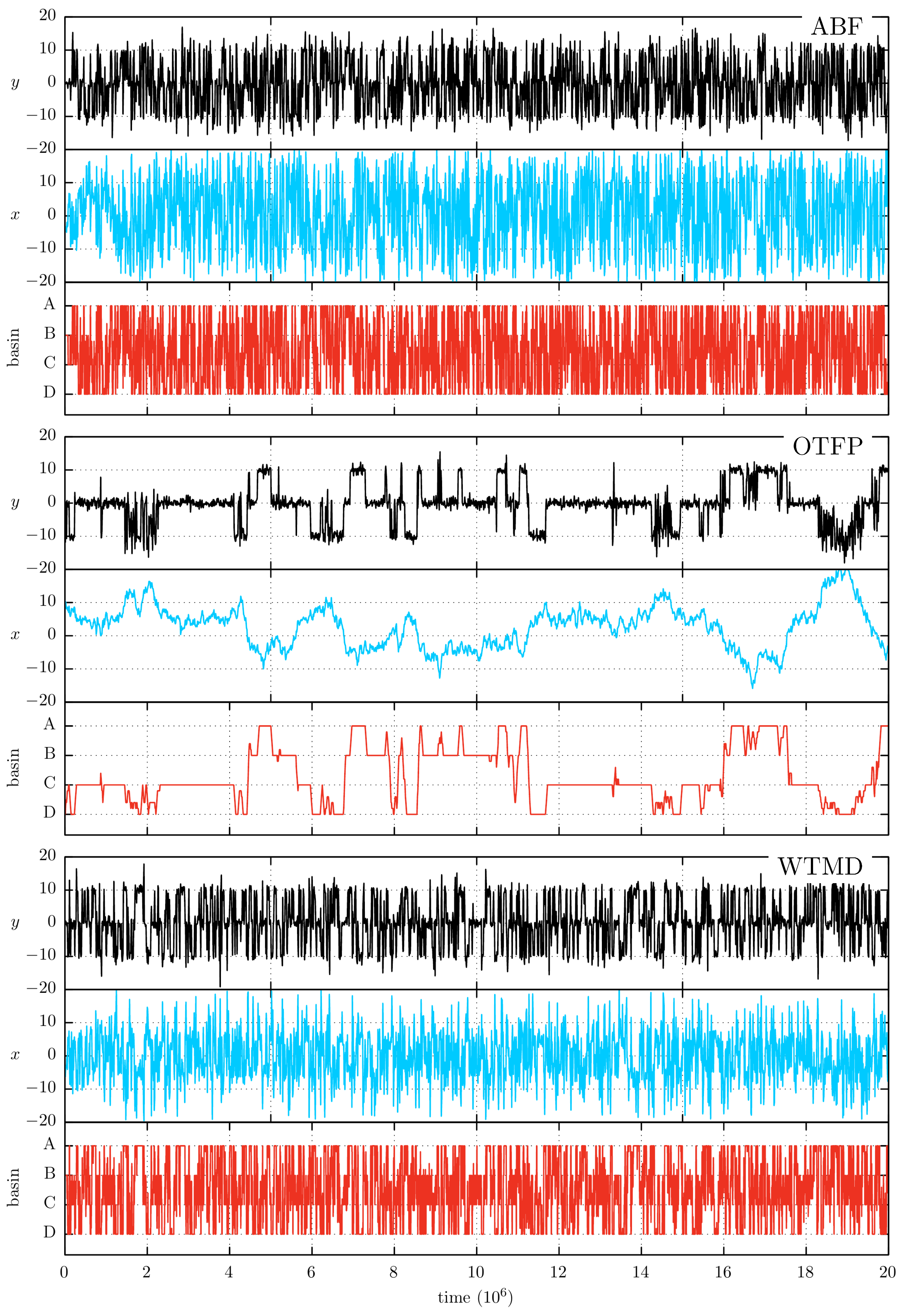
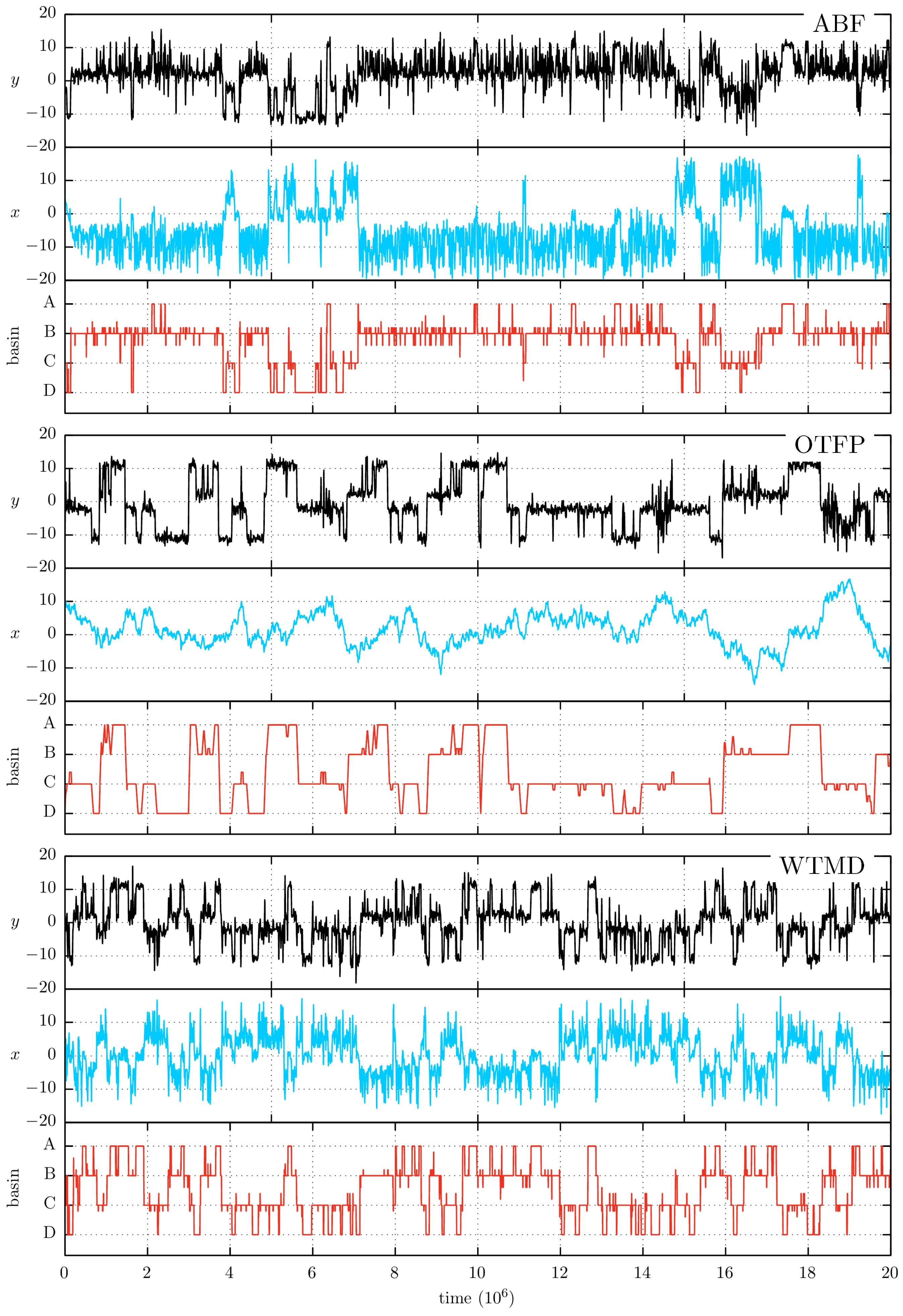
In Figure 4 we show the sampling trace of a representative simulation for each method. In a first analysis of this figure, it is possible to see that the three methods show a faster sampling of the x CV than the one observed in the MD trace of Figure 2. Furthermore, there is an interesting phenomenon that can be observed by a further comparison between Figure 4 and the MD trace. Despite the fact that the acceleration is only focused on the x coordinate, all three methods are evidently able to accelerate the orthogonal y coordinate. An explanation for this acceleration arises when considering that the transitions and have a higher rate when the reactant density along x increases at high-energy states, as occurs during the CV acceleration. For example, a particular transition path that follows the MEP at will have associated a higher barrier than a transition path that start from in the A basin and goes through the transition state. The latter transition increases its probability when the probability to be in increases, as in the accelerated simulations. Thus, although the MEP is orthogonal to the CV variable, the hidden barrier of our example maintain a certain degree of coupling with the CV. This coupling helps to reduce or nullify the negative effect of the hidden barrier’s presence. Finally, Figure 4 shows that the sampling of OTFP is much slower than the one shown by ABF and WTMD. The origin of this difference resides in their different acceleration strategies. The acceleration sampling of the CV in the OTFP/TAMD approach is made via a high-temperature dynamics of the high-friction auxiliary particle. So this implies a slower motion across x but, as it is demonstrated in the TAMD original paper [17], a higher probability to overcome the associated barriers. On the contrary, the acceleration of ABF and WTMD does not require a higher-friction on x, resulting in the faster sampling shown in the figure.
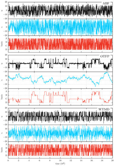
Figure 4.
The position trace of representative ABF, OTFP and WTMD simulations associated with the results shown in Figure 3. For each method, x, y and basin assignation are shown in black, blue and red respectively.
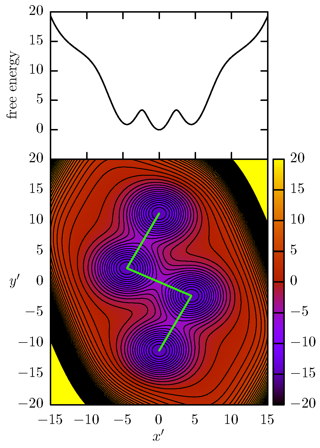
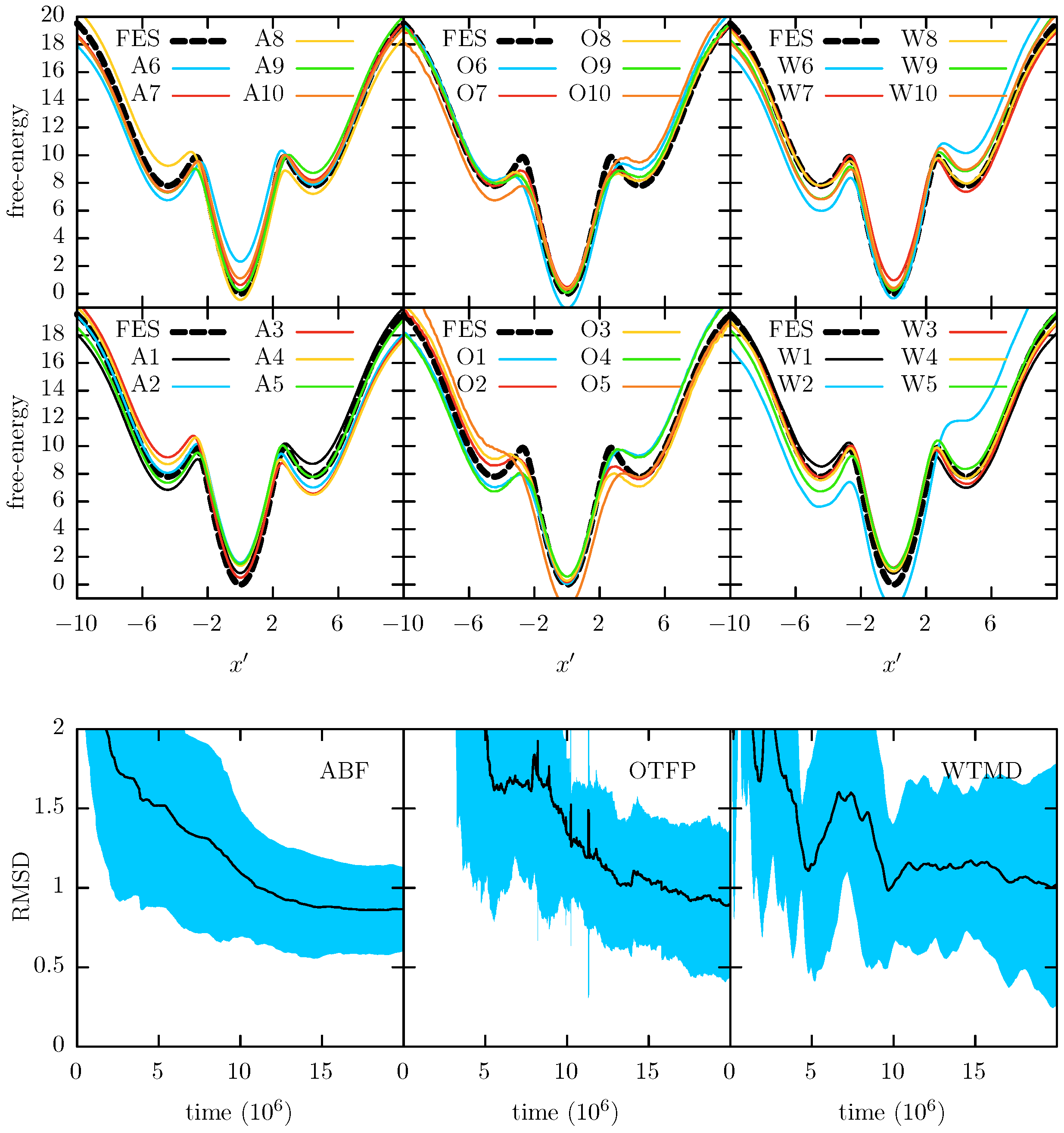
To further investigate the hidden barrier effect on the acceleration methods we change the CV definition by introducing a small rotation of degrees to obtain a coordinate system, , and using as a CV. In Figure 5 it is possible to see the impact of this slight change on the FEP. It is remarkable the significant change generated in the FEP while only this slight CV rotation has been introduced: now the CV shows three FEP minima. However more remarkable is the effect that this small CV change has in the sampling of the free-energy methods. Figure 6 shows the free-energy and convergence profiles for the ABF, OTFP and WTMD simulations. It is possible to see in these plots a performance drop relative to the previous results for the x CV, which is more significant for the ABF and WTMD methods. In Figure 7 we show the trace of some representative simulations. In this figure we can see that ABF gets stuck in an region almost the entire simulation time. On the other hand, WTMD sampling is also affected, showing some periods of being stuck, although less significant than in ABF. Finally, OTFP does not seem to be affected by the CV change and no “sticking” behavior is observed.

Figure 5.
PES and its FEP along the rotated coordinate. To facilitate the vizualizing of the free-energy projection, coordinate is align in the horizontal axis.
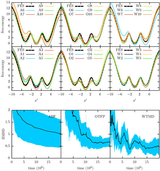
Figure 6.
FEPs obtained using as CV and 10 different simulations for each free energy method as indicated: A1–A10 for ABF, O1–O10 for OTFP and W1–W10 for WTMD. The average convergence profiles are also shown in the bottom of the figure. The light blue region corresponds to one standard deviation. This profiles shows the expected convergence of each individual simulation and should not be confused with the convergence of the average FEP profile. For the average FEP and the individual convergence profiles see Figure S8 in the Supplementary Materials.
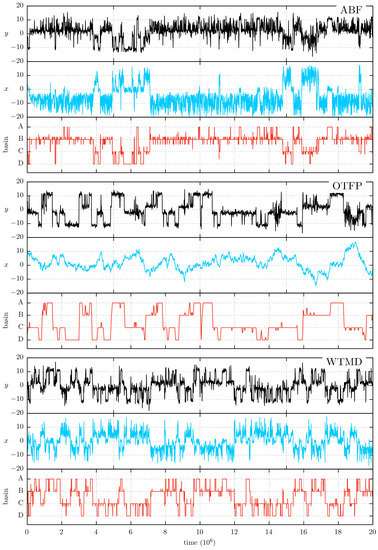
Figure 7.
The position trace of representative ABF, OTFP and WTMD simulations associated with the results shown in Figure 6. For each method, x, y and basin assignation are shown in black, blue and red respectively.
The convergence behavior of WTMD and ABF has been formally analyzed in [18,19,20] respectively. In particular, Lelievre et al. [20] addressed the so-called “bi-channel” case, where there are two different free-energy channels along the CV separated by hidden barriers. They provide a formal treatment of this case and shows that the ABF convergence for this case will depend on the Boltzmann sampling trough the hidden barriers. This is the best scenario that we can expect for any of the methods treated in this work: since the hidden barriers are not being accelerated, their associated transitions will be the lowest modes needed to sample in order to reconstruct the correct FES with the contributions of all the PES metastable states. However, the conclusion achieved by Lelievre et al. is tied to the hypothesis that the (negative) free-energy is a “good bias” in each free-energy channel [20].
We can consider the PES used in this work to be composed of three channels: the region of the transition, with the other two channels leading to the A and D minima. In this scenario, the convergence issue observed for the CV in respect to the x CV can be understood following Lelievre et al. [20]. While the FEP associated with x CV can be considered a good bias for each channel, the FEP associated with is not. The free-energy minima at will result in a high-energy bias that will overlap the energy barrier of the channel. Thus, the ABF and WTMD bias contribute to the barrier at rather than improving the sampling along it, as it is shown in Figure 8. As with many other adaptive importance-sampling techniques, we can expect the same issue to be present in WTMD simulations (see for instance remark 6 of the reference [19] by Lelievre et al.). However, since OTFP is not an adaptive technique, we should not expect to be a priori any further sampling issue, besides the associated with the natural slow sampling of the hidden barriers.
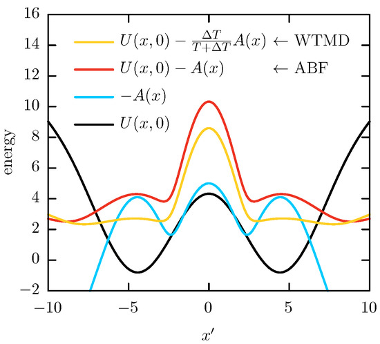
Figure 8.
An scheme to show the prejudicial effect of the bias potential for the middle channel transitions in the adaptive methods. In opposition to reduce the energy barrier at the bias applied by ABF and WTMD helps to increase it.
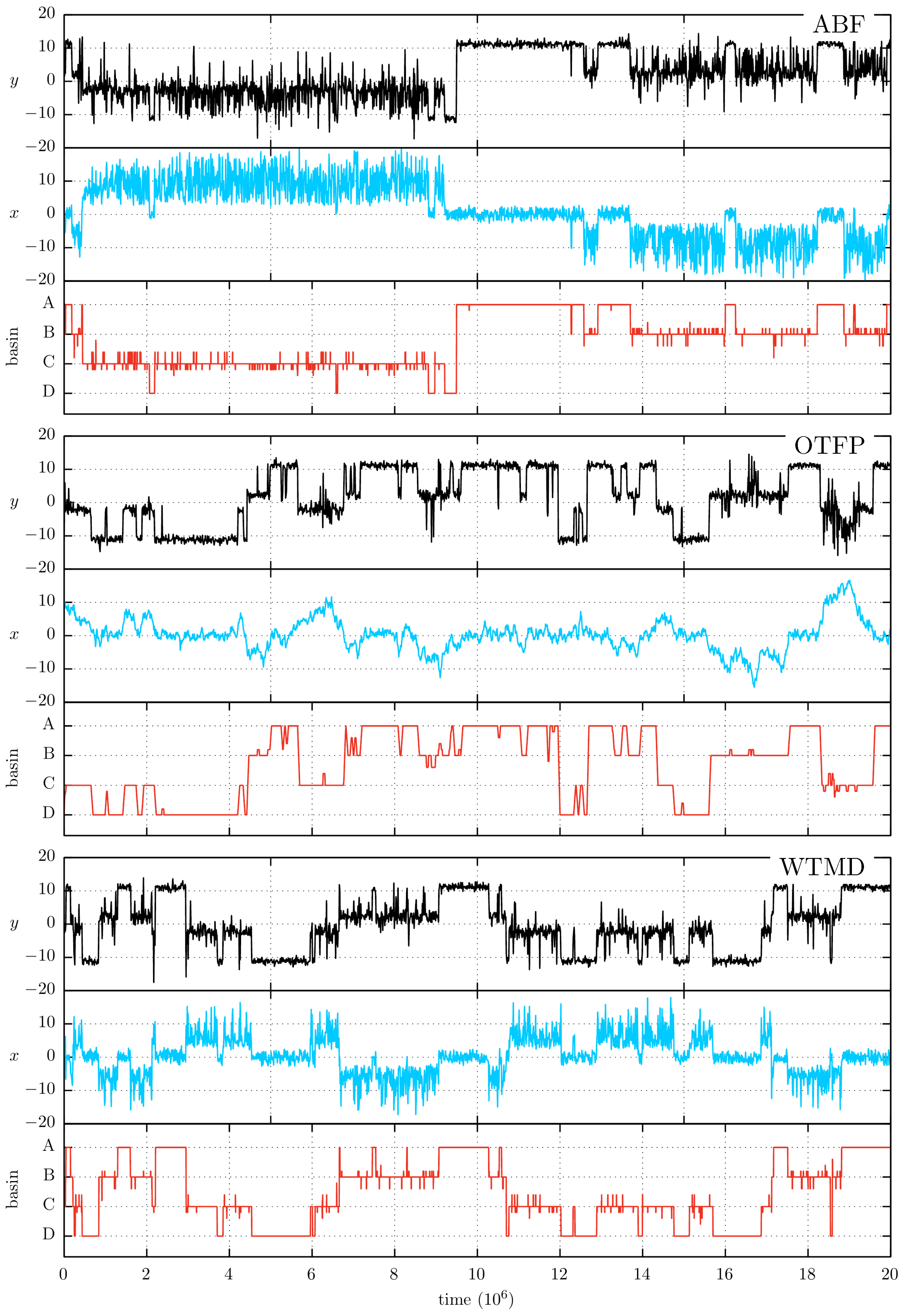
In order to further explore the arguments given in the paragraphs above, we modify the PES by deepening the A and D minima via increasing the and coefficients of Equation (2) from 15 to . Following the above discussion, we expect that this change will have a larger impact in the adaptive methods, since the self-constructed barrier shown in Figure 8 will be increased. The resulting FEP and convergence profiles for are shown in Figure 9. In these plots it is possible to see that the most affected method by this change is WTMD while ABF and OTFP retain the previous convergence behavior. The robust behavior of OTFP is expected from its non-adaptive nature. However, to give an explanation for the impact difference between WTMD and ABF we look to the sampling traces shown in Figure 10. By comparing this figure with Figure 7 it is possible to see that the trapping periods in WTMD trace significantly increase and start to dominate the entire simulation time. For ABF the trapping periods also increase but it already shows a dominance of the trapping periods over the entire simulation time in the previous system. Thus, the deepening of the A and D minima results in breaking the WTMD resistance to the trapping phenomena expected in the adaptive methods. To confirm that the sampling problems in WTMD and ABF arise from the choice of as the CV and not for the solely deepening of A and D minima, we show in Figures S10 and S11 of the Supplementary Materials the results for the x CV. As expected, the three methods are able to recover the corresponding FES for the x CV.
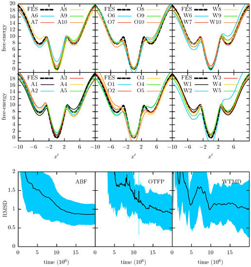
Figure 9.
FEPs obtained using as CV, a deeper A and D PES minima () and 10 different simulations for each free energy method as indicated: A1–A10 for ABF, O1–O10 for OTFP and W1–W10 for WTMD. The average convergence profiles are also shown in the bottom of the figure. The light blue region corresponds to one standard deviation. This profiles shows the expected convergence of each individual simulation and should not be confused with the convergence of the average FEP profile. For the average FEP and the individual convergence profiles see Figure S9 in the Supplementary Materials.
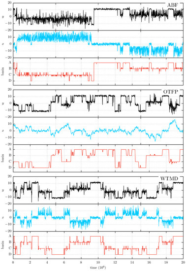
Figure 10.
The position trace of representative ABF, OTFP and WTMD simulations associated with the results shown in Figure 9. For each method, x, y and basin assignation are shown in black, blue and red respectively.
Using the basin trace of all the system studied in this work (see Figure 4, Figure 7, Figure 10 and Figure S11) we have constructed a histogram of the “trapping time” that the system spend in each minimum of the PES and for each method used. This histograms are included in Figures S12–S14 and serves as statistical support to the conclusions drawn in the paragraphs above.
4. Conclusions
We explored the convergence behavior of ABF, WTMD and OTFP in the presence of hidden barriers in three different systems with different degrees of sampling challenges. For the simplest case, we found that the presence of hidden barriers is not enough to generate a negative effect in the free-energy method sampling. Even when the transition associated with these hidden barriers is orthogonal to the CV, the enhancing of the reactant distribution towards high energy regions can improve their sampling. However, for the case of the adaptive importance-sampling technique, such as ABF or WTMD, the CV position of the metastable states associated with the hidden barriers has a crucial role in their sampling behavior. This observation was rationalized in the convergence analysis of Lelievre et al. [20], who showed that the convergence of this methods is guarantee under the condition that the FEP has to be a good bias on each “channel” of the PES, i.e., the sets of metastable states connected along the CV and interconnected by hidden barriers.
By the examples analyzed in this work, we have shown that a slight change in the CV definition is enough to modify the projected position of the metastable states and generate the above mentioned sampling issues. Finally, despite OTFP showing a slower convergence in comparison with the adaptive sampling methods for the simplest system, where the hidden-barriers play a marginal role, it is able to retain its sampling and acceleration behavior in the most difficult cases studied. The robustness shown by OTFP when comparing its convergence across the different systems studied is explained by the fact that OTFP is not an adaptive sampling technique and it does not require a special condition for the different PES channels. This characteristic makes OTFP a tool of choice when hidden barrier are suspected.
Supplementary Materials
The following are available online at http://www.mdpi.com/2079-3197/6/2/27/s1, Figure S1: Minimum Energy Path. Figure S2: MD trajectory at different temperatures. Figures S3–S6: Convergence profiles and FEPs for WTMD and OTFP using different simulation parameters and the x and CV. Figures S7–S9: Convergence profiles and average FEP for Figure 3, Figure 6 and Figure 9 of the manuscript, respectively. Figure S10: FEPs and average convergence for system and using CV x. Figure S11: Position and basin trace of Figure S10. Figures S12–S14: Histogram of trapping times for the traces of Figure 4, Figure 7 and Figure 10 of the manuscript.
Acknowledgments
C.F.A. acknowledges support from the National Science Foundation (DMR-1207389), the National Institutes of Health (R01 GM100472), and the US Army Research Laboratory (W911NF-12-2-0022 and W911NF-12-R-0011).
Author Contributions
S.A.P. and C.F.A. conceived and designed the experiments, performed the experiments, analyzed the data, and wrote the paper.
Conflicts of Interest
The authors declare no conflict of interest.
Abbreviations
The following abbreviations are used in this manuscript:
| ABF | Adaptive-Biasing Force algorithm |
| OTFP | On-the-fly Parameterization |
| TAMD | Temperature Accelerated Molecular Dynamics |
| FEP | Free-energy profile |
| PES | Potential energy surface |
| RMSD | Root-mean-square deviation |
References
- Ciccotti, G.; Vanden-Eijnden, E. The trees and the forest. Eur. Phys. J. Spec. Top. 2015, 224, 2515–2518. [Google Scholar] [CrossRef]
- Abrams, C.F.; Bussi, G. Enhanced Sampling in Molecular Dynamics Using Metadynamics, Replica-Exchange, and Temperature-Acceleration. Entropy 2014, 16, 163–199. [Google Scholar] [CrossRef]
- Torrie, G.M.; Valleau, J.P. Nonphysical sampling distributions in Monte Carlo free-energy estimation: Umbrella sampling. J. Comput. Phys. 1977, 23, 187–199. [Google Scholar] [CrossRef]
- Ciccotti, G.; Kapral, R.; Vanden-Eijnden, E. Blue moon sampling, vectorial reaction coordinates, and unbiased constrained dynamics. ChemPhysChem 2005, 6, 1809–1814. [Google Scholar] [CrossRef] [PubMed]
- Marinari, E.; Parisi, G. Simulated tempering: A new Monte Carlo scheme. Europhys. Lett. 1992, 19, 451. [Google Scholar] [CrossRef]
- Hansmann, U.H. Parallel tempering algorithm for conformational studies of biological molecules. Chem. Phys. Lett. 1997, 281, 140–150. [Google Scholar] [CrossRef]
- Sugita, Y.; Okamoto, Y. Replica-exchange molecular dynamics method for protein folding. Chem. Phys. Lett. 1999, 314, 141–151. [Google Scholar] [CrossRef]
- Barducci, A.; Bussi, G.; Parrinello, M. Well-Tempered Metadynamics: A Smoothly Converging and Tunable Free-Energy Method. Phys. Rev. Lett. 2008, 100, 020603. [Google Scholar] [CrossRef] [PubMed]
- Barducci, A.; Bonomi, M.; Parrinello, M. Metadynamics. Wiley Interdiscip. Rev. Comput. Mol. Sci. 2011, 1, 826–843. [Google Scholar] [CrossRef]
- Paz, S.A.; Abrams, C.F. Free Energy and Hidden Barriers of the β-Sheet Structure of Prion Protein. J. Chem. Theory Comput. 2015, 11, 5024–5034. [Google Scholar] [CrossRef] [PubMed]
- Abrams, C.F.; Vanden-Eijnden, E. On-the-fly free energy parameterization via temperature accelerated molecular dynamics. Chem. Phys. Lett. 2012, 547, 114–119. [Google Scholar] [CrossRef] [PubMed]
- Darve, E.; Rodríguez-Gómez, D.; Pohorille, A. Adaptive biasing force method for scalar and vector free energy calculations. J. Chem. Phys. 2008, 128, 144120. [Google Scholar] [CrossRef] [PubMed]
- Phillips, J.C.; Braun, R.; Wang, W.; Gumbart, J.; Tajkhorshid, E.; Villa, E.; Chipot, C.; Skeel, R.D.; Kalé, L.; Schulten, K. Scalable molecular dynamics with NAMD. J. Comput. Chem. 2005, 26, 1781–1802. [Google Scholar] [CrossRef] [PubMed]
- Hénin, J.; Fiorin, G.; Chipot, C.; Klein, M.L. Exploring Multidimensional Free Energy Landscapes Using Time-Dependent Biases on Collective Variables. J. Chem. Theory Comput. 2010, 6, 35–47. [Google Scholar] [CrossRef] [PubMed]
- Comer, J.; Gumbart, J.C.; Hénin, J.; Lelievre, T.; Pohorille, A.; Chipot, C. The adaptive biasing force method: Everything you always wanted to know but were afraid to ask. J. Phys. Chem. B 2015, 119, 1129–1151. [Google Scholar] [CrossRef] [PubMed]
- Paz, S.A.; Vanden-Eijnden, E.; Abrams, C.F. Polymorphism at 129 dictates metastable conformations of the human prion protein N-terminal beta-sheet. Chem. Sci. 2017, 8, 1225–1232. [Google Scholar] [CrossRef] [PubMed]
- Maragliano, L.; Vanden-Eijnden, E. A temperature accelerated method for sampling free energy and determining reaction pathways in rare events simulations. Chem. Phys. Lett. 2006, 426, 168–175. [Google Scholar] [CrossRef]
- Dama, J.F.; Parrinello, M.; Voth, G.A. Well-tempered metadynamics converges asymptotically. Phys. Rev. Lett. 2014, 112, 240602. [Google Scholar] [CrossRef] [PubMed]
- Lelièvre, T.; Rousset, M.; Stoltz, G. Long-time convergence of an adaptive biasing force method. Nonlinearity 2008, 21, 1155–1181. [Google Scholar] [CrossRef]
- Lelièvre, T.; Minoukadeh, K.; Lelievre, T.; Minoukadeh, K. Long-time convergence of an Adaptive Biasing Force method: The bi-channel case. Arch. Ration. Mech. Anal. 2011, 202, 1–34. [Google Scholar] [CrossRef]
© 2018 by the authors. Licensee MDPI, Basel, Switzerland. This article is an open access article distributed under the terms and conditions of the Creative Commons Attribution (CC BY) license (http://creativecommons.org/licenses/by/4.0/).

