Article

Image Segmentation for Cardiovascular Biomedical Applications at Different Scales

by
Alexander Danilov
1,*,
Roman Pryamonosov
1,† and
Alexandra Yurova
1,2,†
1
Institute of Numerical Mathematics, Russian Academy of Sciences, Gubkina 8, 119333 Moscow, Russia
2
Faculty of Computational Mathematics and Cybernetics, Lomonosov Moscow State University, Leninskie Gory 1, 119991 Moscow, Russia
*
Author to whom correspondence should be addressed.
Computation 2016, 4(3), 35; https://doi.org/10.3390/computation4030035
Submission received: 30 June 2016 / Revised: 27 August 2016 / Accepted: 5 September 2016 / Published: 15 September 2016
(This article belongs to the Special Issue Multiscale and Hybrid Modeling of the Living Systems)

Abstract

:
In this study, we present several image segmentation techniques for various image scales and modalities. We consider cellular-, organ-, and whole organism-levels of biological structures in cardiovascular applications. Several automatic segmentation techniques are presented and discussed in this work. The overall pipeline for reconstruction of biological structures consists of the following steps: image pre-processing, feature detection, initial mask generation, mask processing, and segmentation post-processing. Several examples of image segmentation are presented, including patient-specific abdominal tissues segmentation, vascular network identification and myocyte lipid droplet micro-structure reconstruction.

Graphical Abstract

1. Introduction

Numerical modeling in biomedical applications has remained a challenge for many years. Individualized numerical simulations of physiological processes in the human body received a great deal of attention over several decades, and a vast number of models have been described in the literature. Contemporary resolution of medical images and new algorithms for their post-processing allow us to develop high resolution numerical models of various processes at cellular-, organ-, and whole organism-levels [1,2,3,4,5]. Given an imaging dataset, one performs image segmentation, volume reconstruction, and numerical discretization. In this paper, we present and develop methods and algorithms for construction of patient-specific and cellular micro-structure discrete geometric models for cardiovascular biomedical applications.
The cornerstone of medical image processing is the segmentation process that assigns labels to the voxels. Each biomedical application imposes specific restrictions on both the input medical images and the output patient-specific model, and, therefore, calls for a specific class of 3D segmentation methods. Various medical image segmentation techniques have been developed [6,7,8]. The most promising fully automatic segmentation methods belong to the class of atlas-based segmentation techniques [9,10,11]. The patient-specific segmentation is obtained from the atlas of presegmented images of other individuals. This atlas should contain enough different cases for accurate mapping of the new patient data. Thus, the atlas-based approach requires a huge amount of expert segmentation for preparation of atlases and development of algorithms dealing with big data. The application area of atlas-based methods is limited due to lack of the specialized presegmented atlases. Semi-automatic or supervised segmentation technologies require interaction with the expert. They are used primarily for segmentation of particular organs and tissues.
In this paper, we focus on two cardiovascular applications: haemodynamics and electrophysiology modeling. One can consider the cardiovascular modeling at different scales. The electrocardiography (ECG) forward calculations require the patient-specific segmented thoracic model [12,13]. The bidomain electrophysiology simulation requires the detailed model of the heart ventricles and atria. Whole body haemodynamics modeling requires the full blood vessel network [3,4,14]. Local haemodynamics modeling requires the patient-specific local reconstruction of coronary and cerebral arteries [15,16]. The analysis of internal structure of cardiac cells requires the volume reconstruction of micro-structures [17]. Different image acquisition and segmentation techniques are used in these applications.
In this study, we address several segmentation techniques for contrast-enhanced Computed Tomography (ceCT), contrast-enhanced Computed Tomography Angiography (ceCTA), and Electron Microscopy (EM) images. The overall pipeline for reconstruction of biological structures in cardiovascular applications consists of the following common steps: image pre-processing, feature detection, initial mask generation, mask processing, and segmentation post-processing. The pre-processing step is usually used to smooth the input data and filter noise. Feature detection is a very application-specific step: we use textural features [18] for segmentation of parenchymal organs and vesselness filter [19] for arteries segmentation. We also utilize different mask generation, mask processing, and segmentation post-processing methods in our applications: the level set methods [20] are used for parenchymal organs, and isoperimetric distance trees [21] and distance ordered homotopic thinning [22,23] are used in vessel segmentation. The modality- and structure-specific features of segmentation process are presented in detail in this work.
Various segmentation methods are used for generation of discrete models suitable for ECG forward calculations. In our previous work, we used several techniques for adaptation of the segmented reference human model to different individuals. This technique relies on anthropometric scaling, control points mapping and supervised segmentation [24,25]. We extend our segmentation techniques for electrophysiology modeling and ECG forward calculations with heart ventricles and the atria supervised segmentation method [26]. In this paper, we evaluate several ideas for automatic segmentation of thorax and abdominal tissues using ceCT images in order to improve ECG modeling.
Our previous technique of coronary artery segmentation and graph network reconstruction for haemodynamics modeling [23] is improved and extended for both coronary and cerebral arteries using ceCTA. This technique reconstructs both the 3D segmented image and 1D centerlines network. The segmented image may be used for 3D discrete mesh generation, and the 1D vessels network may be used in 1D haemodynamics modeling. The improved algorithm for coronary artery segmentation includes an additional aorta border cleaning step. The cerebral artery segmentation method is designed in the same way as in [23,27,28].
There are several approaches for cerebral artery segmentation. Some of them [29,30] are focused only on the brain arteries, ignoring neck vessels. Another semi-automatic approach is based on the level set methods [31]. Olivier Cuisenaire, in his work [32], takes advantage of the active objects method, requiring the localization of initial seed points at the vessel ends; user interaction is reduced by the use of a patient-adapted anatomical model. However, in some cases, supervised initialization is still required. Our technique is based on the following idea. First, all arteries in the domain are segmented by the vesselness filter; second, the 1D structure is reconstructed by the thinning process. Thus, blood vessel ends are extracted automatically and no initial seeds are required.
In this work, we discuss the segmentation techniques for reconstruction of cardiac cell micro-structure from EM images. The huge size of typical EM images requires the use of automatic methods. The supervoxels, shape features, and machine learning techniques may be used to reduce the problem sizes and detect specific micro-structures [33]. In our work, we uncovered inhomogeneity in some myocyte lipid droplets; and we applied basic threshold-based methods for reconstruction of internal structure of these lipid droplets.
In this study, we present in detail the segmentation techniques for cardiovascular biomedical applications, the enhanced automatic algorithm for coronary and cerebral arteries segmentation with alternative segmentation correction step, and the reconstruction of inhomogeneous structure of lipid droplets in human myocyte cells.
The paper outline is as follows. In Section 2, we discuss and present segmentation methods for ceCT, ceCTA, and EM images. In particular, we consider segmentation of abdominal parenchymal organs, coronary and cerebral arteries, and myocyte micro-structure. In Section 3, we demonstrate the results of the proposed techniques. Section 4 concludes the paper with discussions.

2. Segmentation Techniques

The bioelectrical inhomogeneities of the human thorax affect the ECG forward calculation. Reconstruction of a fully heterogeneous model remains time-consuming and labor-intensive as a complete automatic segmentation is not available. Recent research on influence of different tissues [34] on ECG signals suggests that muscle, lungs and fat tissues are more important than the others. Most of these tissues can be segmented automatically [35,36,37,38]. In this paper, we will focus on segmentation of abdominal parenchymal organs. The liver is a typical example of these organs. Its size and proximity to the heart indicate noticeable influence on ECG modeling.

2.1. Segmentation of Abdominal Parenchymal Organs

In this part, we propose a method for segmentation of abdominal parenchymal organs. The main steps of the algorithm are binary mask generation using analysis of CT texture features and further extraction of the 3D organ models.
The fully automatic segmentation of abdominal cavity is a complicated task because of several factors. First, there is a large anatomical variability of patients; second, medical images come from different devices and have different properties; third, similar intensity values for adjacent organs make boundary detection difficult. To partly overcome this problem, we considered contrast-enhanced CT as input data. Multiphase CT-scans are performed in order to enhance contrast between anatomical structures. The main phases of enhancement are as follows: without contrast (non-enhanced CT), arterial, portal and late phase. In our research, the smoothed CT-scans of the portal phase are used.
We have experimented with several segmentation techniques. In [39], we proposed a method of the piecewise affine mapping of the segmented reference model. This transformation requires a set of the control points defined on both reference and patient images. Control point localization is a very time-consuming task that requires a good understanding of human anatomy. We have also investigated some strategies based on the voxel clustering [33,40]. The clusterization algorithm takes into account only intensities and distances between voxels. However, the abdominal organs boundaries are not always clear, since the intensity ranges overlap. Therefore, some clusters contain voxels belonging to different tissues. It makes further cluster processing complicated. In addition, parameters of cluster generation highly depend on intensity range of the input image, which makes fully automatic segmentation difficult. We also implemented several methods proposed in [41]. Most of them are based on the gray level analysis and take into account anatomical peculiarities of the patient. These semi-automatic methods are rather good, but are sensitive to dataset variations because of gray levels variability between patients.
We propose a method that is robust to inter-patient gray level and anatomical variability. The main idea is based on two properties of parenchymal organs: homogeneous structure and relatively sharp boundaries on the images with contrast. We use texture analysis to measure these properties. In [18], some texture features were proposed for 2D image classification. We used these ideas for segmentation of 3D medical images.
Textural features are computed using s × s × s voxel neighborhood, where s is an odd number greater than 1. In our study, we considered several textural features: contrast, inverse difference moment, second angular moment, etc. From all experimental results, the entropy was chosen as the most informative and easily processed. It is easy to verify that the range of entropy values is [ 0 ; ln n ( s ) ] , where n ( s ) = 6 × ( s - 2 ) 3 + 5 × 6 × ( s - 2 ) 2 + 4 × 12 × ( s - 2 ) + 3 × 8 , is the doubled number of connections in the cubic neighborhood. Let p be the spatial-dependence matrix [18], p ( i , j ) be its ( i , j ) entry. One can prove that entropy
E N T = - i , j p ( i , j ) ln ( p ( i , j ) )
achieves its maximum value ln n ( s ) , if the number of different adjacent voxel pairs is equal to the number of connections in the neighborhood.
This entropy property describes two important anatomical peculiarities used for segmentation process in this study: voxels inside of parenchymal organs have low entropy values because of the homogeneous structure and voxels of the boundary have high values because of diversity of intensities in the neighborhood.
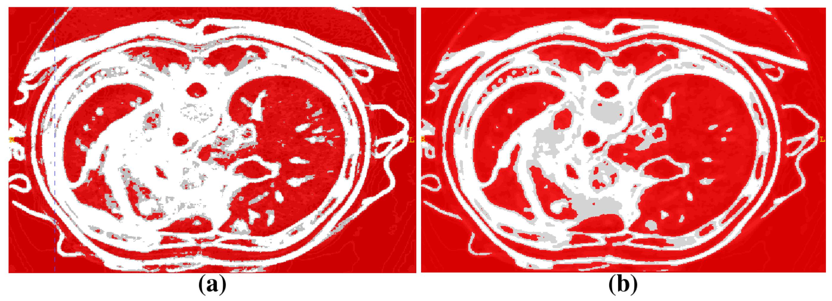
Figure 1 demonstrates the result of entropy computation for different neighborhood sizes ( s = 3 , 5 ). Experiments with different datasets have shown that the 3 × 3 × 3 voxel neighborhood ( s = 3 ) is sufficient for parenchymal organs detection. In this case, n ( 3 ) = 108 and E N T [ 0 , 5 ) . Using thresholding, we can obtain the corresponding binary masks (rf. Figure 2). Analyzing a histogram, we have selected thresholds for s = 3 equal to three and verified it experimentally with CT images of different patients. This threshold value provides rather good results for different datasets.
The second step of our algorithm is 3D volume extraction. Binary mask does not represent organs as separated components because of the multiple “leaks”. We use active contours method for extraction of parenchymal organs. We compared several implementations of active contours methods [20,42,43]. The most convenient one for our purposes is the level set function implemented in Convert3D tool from ITK SNAP (Philadelphia, PA, USA) ([44]). The coordinates of seed points can be found automatically using prior anatomical knowledge.
The evolution of closed surface C ( u , v ; t ) is governed by the equation:
C t = ( α g I - β κ ) n ,
where n is the unit normal vector to the contour. Two forces act on the contour in the normal direction: α g I is the internal force (the propagation term) and β κ is the external force (the spatial modifier term), where κ is the mean curvature of the contour, g I is the speed function computed from the input image, and α, β are scalar constants. Equation (2) describes the velocity of every point of the contour at any moment of time. The propagation term is proportional to the values of the feature image, computed from the input image voxelwise by some function. The advantage of our method is that the binary mask from the previous step is used directly as a feature image eliminating the necessity to compute it explicitly. The spatial modifier term controls the smoothness of the evolving contour and is approximately proportional to the curvature of the contour at the point.
Relation between forces can be controlled by setting appropriate parameters. One can easily change parameters and observe regions growing using ITK SNAP user graphical interface (Active Contour Segmentation Mode, [44]). To avoid contour evolution into neighboring structures, we have to maintain a certain smooth shape by setting the spatial modifier term significantly bigger than the propagation term: 0.9–1.0 and 0.1–0.25, respectively. One can slow down contour evolution into domains with high curvature and effectively smooth organ surfaces.
The summary of our algorithm for parenchymal organs segmentation is presented below:
  • Pre-process and smooth the input dataset.
  • Compute the spatial-dependence matrix (specified in [18]) for all voxels of the smoothed dataset.
  • Compute entropy (1) for each voxel using the spatial-dependence matrix.
  • Obtain the binary mask by entropy values thresholding.
  • Set the seed points for organs extraction.
  • Implement active contours method and extract 3D model.
The results of the proposed segmentation technique are presented in Section 3. This algorithm is especially useful for segmentation of a liver, which is one of the significant organs during ECG modeling.

2.2. Vessel Segmentation

In this section, we propose algorithms for automatic segmentation of coronary and cerebral human arteries. We assume that the input data is a 3D DICOM (Digital Imaging and Communications in Medicine) dataset acquired using ceCTA protocol. All algorithms presented in this section are developed for uniform cubic voxel grids; the anisotropic dataset should be resampled prior to segmentation. We also assume that each voxel has 26 adjacent voxels, i.e., voxels with common face, edge or vertex.
Both segmentation techniques are based on the Isoperimetric Distance Trees (IDT) algorithm [21] and Frangi Vesselness filter [19]. Output segmentations are represented by the binary masks that are useful for skeletonization post-processing.
Algorithms for coronary and cerebral cases are almost similar and consist of next essential steps:
  • Segment the aorta.
  • Remove pulmonary arteries.
  • (Cerebral case only) Darken bone intensities.
  • Apply Frangi Vesselness filter.
  • Locate the ostia points or aortic arch branches and segment the vessels.
  • Clean aorta border.
The aorta segmentation algorithm was presented in our previous work [23]. In the current work, we extend this algorithm to cerebral datasets. Pulmonary arteries are removed by the morphological operations proposed in [27]. Bone elimination is an essential step for cerebral artery segmentation due to vertebral arteries and cervical vertebrae proximity. Assuming both CT and ceCTA datasets are available for the same patient, bones can be automatically darkened with the multiscale matched mask bone elimination algorithm [45]. Otherwise, bones should be segmented and eliminated manually. Ostia points are detected as two distant vesselness maxima near aorta border. Aortic arch branches are defined as connected components of voxels with high vesselness, lying close to aorta border. Aorta border cleaning is the final step, which is necessary since high vesselness values may falsely occur near big bright structures.
We employ the IDT algorithm for aorta segmentation, since aorta is much larger than coronary or cerebral vessels and its segmentation using vesselness filtering is very time consuming. The IDT method starts from the binary mask M i n i t and a voxel c, it cuts the mask M i n i t through bottlenecks and outputs submask M A containing c. Full automatic aorta segmentation can be achieved with the Circle Hough Transform (CHT) [46] (we use its implementation in ITK library [47]). The transform is used to detect the largest bright disk D and its radius R A on transverse planes. This disk is an aorta cross-section. Initial mask is acquired by thresholding method with a minimal intensity inside of the disk t i n i t as a threshold parameter. The center of the disk is considered as the initial voxel c.
After the IDT stage, some parts of aortic arch branches or coronary arteries may still be included in M A . In the coronary case a simple morphological smoothing of M A is sufficient in order to remove coronary parts and to keep the mask intact. However, carotid and subclavian arteries are bigger than the coronary arteries and thus algorithm requires more sophisticated approach for their removal.
To this end, we define mask smoothing with parameter p as successive deletion of p voxels thick border from the mask (p-border) and addition of p-border. Details of the smoothing method are discussed in [23]. We should note that the smoothing procedure with high parameter values distorts input masks. Next, we use three parameters r, R, t to remove coronary and cerebral arteries from the aorta mask M A . The specific values of these parameters are presented in Section 3. We assume the mask M A is already smoothed with a parameter r and coronary vessels are already excluded. In order to remove the aortic arch branches, the mask M A is copied to the mask M s m o o t h and M s m o o t h is smoothed with high parameter R. After that step, M s m o o t h is distorted but no longer contains any parts of carotid or subclavian arteries. We add t-border to the mask M s m o o t h and intersect it with the mask M A . The last step allows the resulting mask to keep intact the border of the mask M A . To summarize, we refer the reader to the next algorithm:
  • Compute the radius and the center c of the largest bright disk D on transverse planes using CHT method.
  • Construct the connected region mask M i n i t containing voxel c with the minimal intensity inside of D as the lower threshold.
  • Obtain M A as a result of the IDT method applied to the mask M i n i t and the seed c.
  • Smooth the mask M A with the parameter r.
  • (Cerebral case only) Copy mask M A to mask M s m o o t h . Delete R-border from M s m o o t h , then add ( R + t ) -border.
  • (Cerebral case only) Intersect the mask M A with the mask M s m o o t h .
Frangi vesselness filter is a useful instrument for vessel segmentation since it results in high vesselness values inside of the vessels and low values elsewhere. However, the filter may also produce high values near large bright structures like aorta. Authors of [27] proposed the modified vesselness function; however, we observed false filter response only near the aorta, and, thus, we propose an alternative approach for segmentation correction only near the aorta border. It should be noted that conventional remove-islands procedure may not eliminate the segmentation errors since false regions are attached to the arteries.
We define distance map d m a p M ( v ) as the distance to the mask M for each voxel v. The detailed description of distance maps and its construction process are presented in [23]. We assume the mask M V represents the vessels, and the mask M A represents only the aorta. We define the voxel layer L d = { v M V | d m a p M A ( v ) = d } as a subset of mask M V distanced from the mask M A by the distance d. Note that distance is measured in voxels, and it depends on the metric used in distance map construction. For each voxel layer L d for d = d max , , 0 we apply the following procedure: remove all voxels from L d that have no adjacent voxels in L d + 1 . The parameter d max should be big enough, so that voxel layer L d max contains no segmentation errors. In our practice, we set d max = 15 .

2.3. Segmentation of Lipid Droplets

In this paragraph, we discuss a specific technique for segmentation of internal structure of lipid droplets in human myocyte cells. The myocyte 3D structure is obtained by electron microscopy (EM) that is a key technique to observe tissues on cellular level. One of the EM techniques is a 3D focused ion beam (FIB) method. FIB is applied to the tissue, which was previously embedded and repeatedly milled layer by layer (each about 10 nm thick). These layers may shift during the procedure, hence all segmentation techniques for EM-FIB data require preliminary slice alignment. For additional details on the FIB method, we refer to [17].
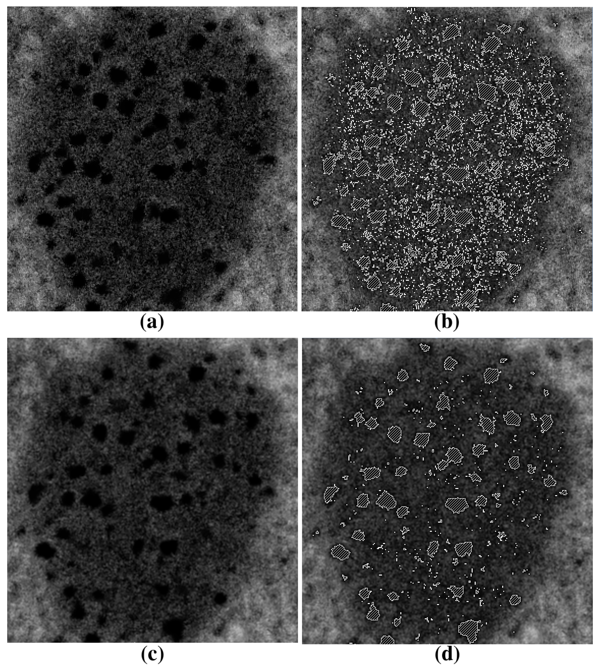
The shape of lipid droplets may be easily extracted using threshold method and edge detector [17], since the lipids have the lowest intensities in the FIB images. The internal structure of some inhomogeneous lipid droplets is noticeable by detailed examination. Figure 3 demonstrates the region containing lipid droplet. This region was cropped from the original EM-FIB data provided by I.R. Efimov of the George Washington University, Department of Biomedical Engineering (Washington, DC, USA).
The structure of the lipid droplets is represented by two intensity ranges: darker intensities represent the inhomogeneous inclusions, and slightly brighter ones determine the shape of the lipid droplet. A naive thresholding approach may produce incorrect results due to different sharpness of 2D image slices. Some of the slices are sharp with low signal-to-noise ratio (SNR), and the others are blurred. We noticed that threshold may be applied successfully only in the case of the smoothed images. Taking it into account, one can smooth the sharp 2D slices and threshold all slices eventually, producing satisfying results. Alternatively, one can apply the 3D Gaussian smoothing to the whole lipid droplet region rather than search for the sharp 2D slices manually. The remove-islands procedure is applied as a final post-processing step. This procedure removes the disconnected regions with volume lower than the parameter threshold.
All steps may be formalized in the next algorithm:
  • Align all 2D slices of the image dataset.
  • Detect all lipid droplets using the threshold method (ref. [17]).
  • Apply Gaussian smoothing in the vicinity of the lipid droplet.
  • Segment inhomogeneous inclusions by thresholding with the lower parameter.
  • Apply 3D remove-islands procedure.
The two threshold parameters correspond to the local minima of the intensity histogram of the cropped FIB dataset (Figure 4). The left peak represents the intensities of the inhomogeneous inclusions, the middle peak represents the intensities inside of lipid droplet, and the right peak represents the intensities of surrounding cell structures. The intensity histogram of the homogeneous lipid droplet does not contain explicit local minimum inside the droplet intensity range.
The cell organelles with easily detectable boundaries and distinct internal structure may be segmented using the similar technique.

3. Results

All proposed methods were implemented in our research code using Python and C programming languages. Several intermediate steps were performed using third-party software packages.
The parenchymal organs segmentation technique was implemented using Python programming language. We demonstrate results of experiments on two DICOM datasets. The first dataset represent normal abdominal CTA in venous phase obtained from DICOM with alias name OBELIX from the OsiriX samples database [48]. The second anonymized DICOM dataset was provided by the staff of I. M. Sechenov First Moscow State Medical University, Moscow, Russia.
The entropy feature computation is a computationally expensive step, thus a separate massive parallel OpenCL-based (Open Computing Language) version of the code was implemented using PyOpenCL package. Both sequential CPU (Central Processing Unit) and parallel GPU (Graphics Processing Unit) versions were tested. Intel Core i7 CPU (Santa Clara, CA, USA) was used for CPU version of the code. The GPU version was executed on NVIDIA graphic card GeForce GT 740M (Santa Clara, CA, USA). Both versions result in exactly the same entropy feature distribution, though the GPU version is considerably faster. The computation times of both versions are presented in the Table 1.
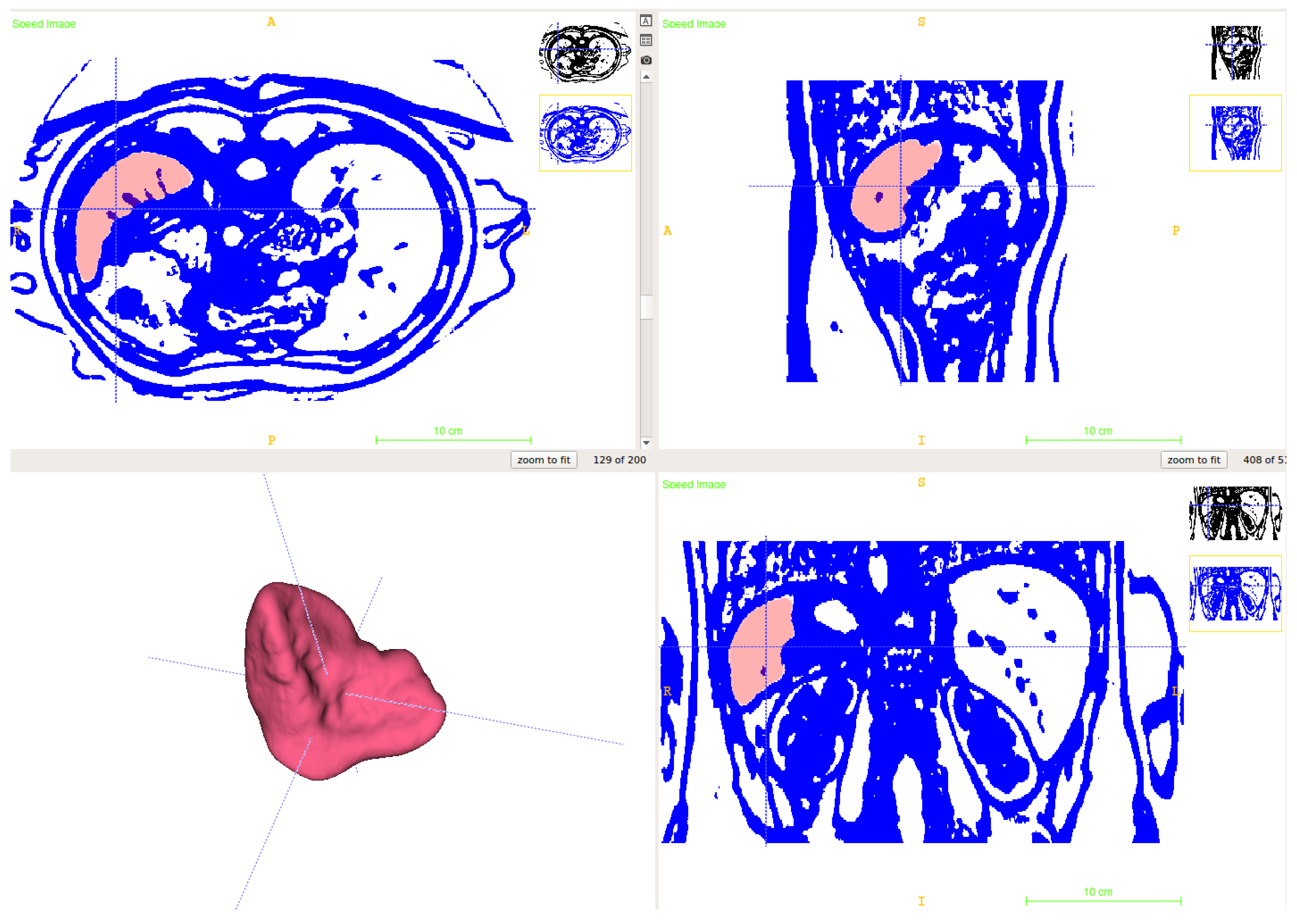
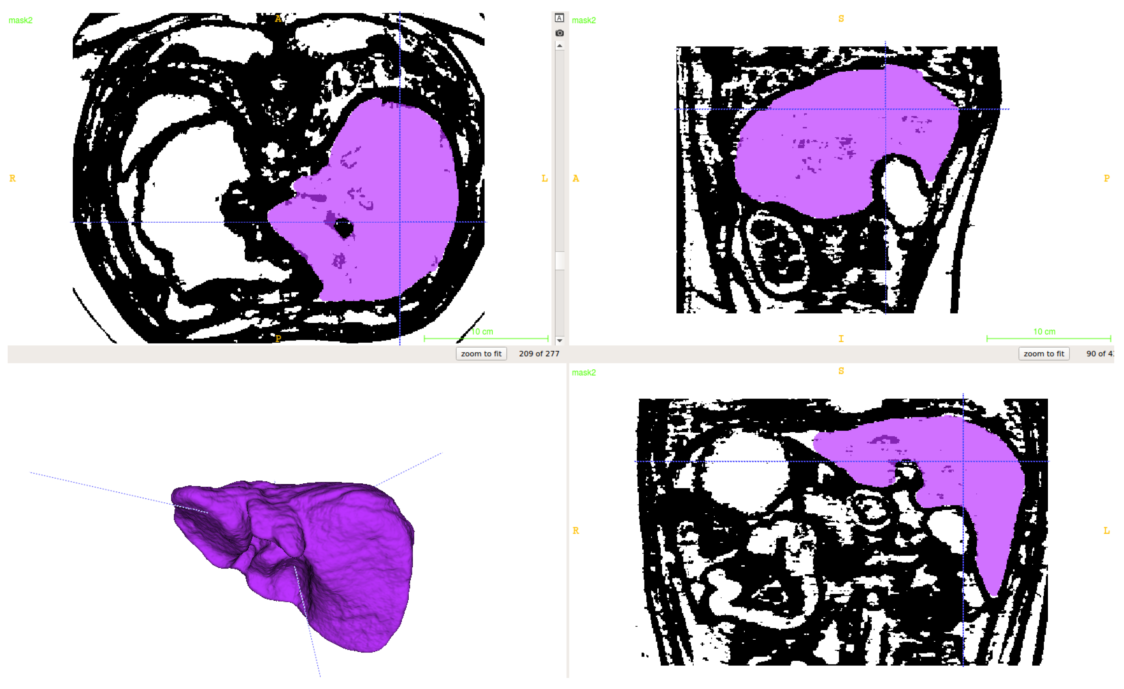
The results of spleen and liver segmentation with parameters α = 0.2 , β = 0.95 from (2) are presented in Figure 5 and Figure 6. The 3D model generation was performed using ITK SNAP software (version 3.4.0, University of Pennsylvania, Philadelphia, PA, USA) [44].
The vessel segmentation algorithms were tested on several coronary and cerebral ceCTA images. Anonymized DICOM datasets were provided by the staff of I. M. Sechenov First Moscow State Medical University. Several examples of false vesselness filter responses during segmentation process are presented in Figure 7a–c. The distance map based correction procedure is used as described above for final segmentation (rf. Figure 7c,d).
Cerebral vessels segmentation algorithm was tested on two ceCTA DICOM datasets with resolutions 512 × 512 × 501 voxels and 512 × 512 × 451 voxels and voxel spacing 0.76 × 0.76 × 0.80 mm and 0.62 × 0.62 × 0.80 mm, respectively. Although the original algorithm was designed for cubic voxel grids, the experiments on slightly anisotropic grids show good results.
Bones were removed manually due to lack of non-enhanced CT data. The parameters r, R and t of the aorta segmentation algorithm were set in accordance with experiments to provide anatomically correct results:
r = 1 3 R A , R = 2 3 R A , t = 1 7 R A ,
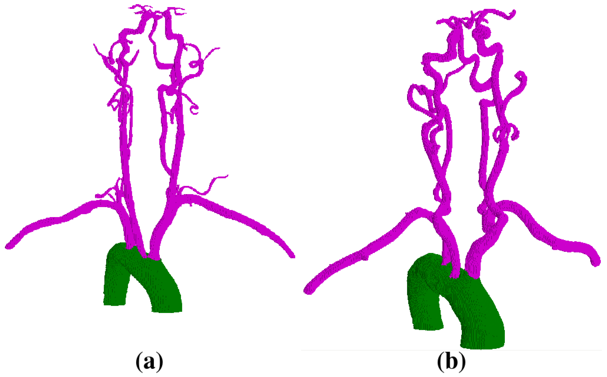
where R A is the actual radius of aorta cross-section estimated by CHT. Frangi Vesselness parameters were set to 0.2 , 0.5 , 500 and filter was computed at scales 1–5 (ref. [23] for details). In both cases, subclavian, carotid, vertebral arteries and the circle of Willis were successfully segmented. Figure 8 demonstrates the results of automatic segmentation. CPU times are presented in Table 2 for the same Intel Core i7 CPU machine.
The vascular network 1D graphs were reconstructed from the segmented images and were used in haemodynamics numerical modeling in the work [49]. The coronary arteries segmentation algorithm was thoroughly tested in our previous works [23,50].
The proposed segmentation technique for reconstruction of the lipid droplets internal structure was tested on the FIB dataset that was produced the same way as in [17]. The original image dataset was cropped to the region of interest, containing only one lipid droplet (rf. Figure 3). The 3D volume of the lipid droplet structure reconstructed by thresholding and post-processing of aligned and smoothed FIB slices is presented in Figure 9. For the last dataset, thresholds were set to 3 and 54, according to the histogram local minima as described above (Figure 4).
The inhomogeneous structure is observed only in some lipid droplets. The causes and effects of these inhomogeneities should be further investigated.
Segmentation of the whole myocyte cell 3D structure is important for understanding of myocardial tissue processes on a cellular level. There are two main points in the segmentation strategy for EM images. First, automation is important for segmentation of EM data because of its large size and cellular structure complexity. Manual or semi-automatic segmentation is very difficult in the EM case. Second, EM images contain a variety of different objects (mitochondria, t-tubules, etc.) with overlapping intensity ranges. It is difficult to segment these structures relying only on the local image statistics. In addition, algorithms based on thresholding are inapplicable in most cases.
Several works were published on EM segmentation [33,51], but none of these algorithms were yet tested with the structure of myocyte cells. These methods are based on two fully automated approaches: clustering and machine learning. According to [40], clustering downsamples the image into supervoxels, meaningful regions that can be used to replace the rigid structure of the voxel grid. Machine learning does not require special knowledge of the object structure and relies on global image statistics. In summary, the combination of these two approaches satisfies both requirements of EM image segmentation and may be applied to all cell structures. Thus, it should be tested on myocyte EM images.

4. Discussion

Image segmentation is a crucial process in biomedical modeling. Complex models require segmentation of complex biological structures. Regardless of the image scale, one can use the thresholding technique, if the structure to be segmented has distinct intensity range. However, when several organs or organelles have overlapping intensity ranges, more complex methods are required. In the case of EM, local image statistics are not sufficient in contrast to vessel or abdominal organs segmentation where local information (vesselness and texture features) provides good results. Examples of the overlapping intensities are presented in this work: bone tissue and arteries in ceCTA, abdominal parenchymal organs in CTA, and organelles of myocyte cells in EM. Examples of distinct intensity ranges are lungs in CTA and lipid droplets in EM.
All of the proposed techniques consist of the following common steps: image pre-processing, feature detection, initial mask generation, mask processing, and segmentation post-processing. These techniques have several limitations. Similar intensity values of adjacent organs make boundary detection difficult in abdominal segmentation; we use portal phase ceCT images to overcome this problem. The vessel segmentation algorithm is designed for cubic voxels and performs well for slightly anisotropic voxel grids; highly anisotropic grids should be resampled prior to the segmentation process. Both CT and ceCTA images are required for automatic cerebral arteries segmentation; an additional supervised preprocessing step is needed in case only ceCTA data are available. Nevertheless, the proposed and discussed techniques and algorithms for CTA, ceCTA and EM images show reasonable applicability for object-specific segmentation on various datasets modalities and scales. These methods extend the applicability of the cardiovascular modeling algorithms. Further improvements allow us to create an automated segmentation framework needed for patient- and object-specific numerical modeling.
The important example of modeling application includes the patient-specific haemodynamics modeling. Automatic and correct segmentation of arteries result in more accurate simulation. Another important cardiovascular application is the ECG forward calculation. Automatic algorithms for segmentation of lungs, muscles, fat tissues, and abdominal organs decrease the uncertainty of numerical ECG models.
As the automatic segmentation techniques will eventually be included in everyday practice, the efficiency and speed of the algorithms will become crucial. Some computationally expensive steps of the segmentation process have a great potential to be accelerated using massive parallel programming on GPU devices. For instance, time effectiveness of the proposed cerebral segmentation algorithm can be improved with a parallel version of Frangi Vesselness, which is computed in each voxel of the 3D dataset. Our preliminary experience in accelerating the processing code using OpenCL technology shows promising results.

5. Conclusions

We presented several techniques of image segmentation for cardiovascular biomedical applications. Segmentation of abdominal parenchymal organs, vessels, and lipid droplets was addressed. The algorithms were designed with automation in mind; user interaction was minimized. The results demonstrated reasonable applicability of the proposed methods to medical image data. OpenCL-accelerated version of the texture-based segmentation algorithm was implemented and tested, showing good computation speed-up. In future work, the segmentation methods will be improved, particularly concerning extension of applications range, inclusion of machine learning techniques, and parallel acceleration.

Supplementary Materials

The 3D volume reconstruction of internal lipid droplet structure (ref. Figure 9) and the segmented models of cerebral arteries are available online at www.mdpi.com/2079-3197/4/3/35/s1. Please note that the research code and DICOM datasets are available upon request.

Acknowledgments

The research was supported by Russian Science Foundation grant 14-31-00024. The authors thank Igor R. Efimov of the George Washington University, Department of Biomedical Engineering, for providing the FIB image dataset. The authors acknowledge the staff of I. M. Sechenov First Moscow State Medical University and especially Philippe Yu. Kopylov, Nina V. Gagarina, Ekaterina V. Fominykh, Andrey N. Dzyundzya for patient-specific data.

Author Contributions

Roman Pryamonosov and Alexandra Yurova developed, implemented and tested the presented segmentation techniques; Alexander Danilov conceived the study and participated in its design and coordination; All authors wrote, read and approved the final manuscript.

Conflicts of Interest

The authors declare no conflict of interest.

References

  1. Dazzo, F.; Niccum, B. Use of CMEIAS Image Analysis Software to Accurately Compute Attributes of Cell Size, Morphology, Spatial Aggregation and Color Segmentation that Signify in situ Ecophysiological Adaptations in Microbial Biofilm Communities. Computation 2015, 3, 72–98. [Google Scholar] [CrossRef]
  2. Kislitsyn, A.; Savinkov, R.; Novkovic, M.; Onder, L.; Bocharov, G. Computational Approach to 3D Modeling of the Lymph Node Geometry. Computation 2015, 3, 222–234. [Google Scholar] [CrossRef]
  3. Sazonov, I.; Yeo, S.Y.; Bevan, R.L.T.; Xie, X.; van Loon, R.; Nithiarasu, P. Modelling pipeline for subject-specific arterial blood flow—A review. Int. J. Numer. Methods Biomed. Eng. 2011, 27, 1868–1910. [Google Scholar] [CrossRef]
  4. Quarteroni, A.; Tuveri, M.; Veneziani, A. Computational vascular fluid dynamics: Problems, models and methods. Comput. Vis. Sci. 2000, 2, 163–197. [Google Scholar] [CrossRef]
  5. Gerbeau, J.F.; Vidrascu, M.; Frey, P. Fluid–structure interaction in blood flows on geometries based on medical imaging. Comput. Struct. 2005, 83, 155–165. [Google Scholar] [CrossRef]
  6. Holtzman-Gazit, M.; Kimmel, R.; Peled, N.; Goldsher, D. Segmentation of thin structures in volumetric medical images. IEEE Trans. Image Proc. 2006, 15, 354–363. [Google Scholar] [CrossRef]
  7. Radaelli, A.G.; Peiró, J. On the segmentation of vascular geometries from medical images. Int. J. Numer. Methods Biomed. Eng. 2010, 26, 3–34. [Google Scholar] [CrossRef]
  8. Yeo, S.Y.; Xie, X.; Sazonov, I.; Nithiarasu, P. Segmentation of biomedical images using active contour model with robust image feature and shape prior. Int. J. Numer. Methods Biomed. Eng. 2014, 30, 232–248. [Google Scholar] [CrossRef] [PubMed]
  9. Rohlfing, T.; Brandt, R.; Menzel, R.; Russakoff, D.B.; Maurer, C.R. Quo Vadis, Atlas-Based Segmentation? In Handbook of Biomedical Image Analysis: Volume III: Registration Models; Springer: Boston, MA, USA, 2005; pp. 435–486. [Google Scholar]
  10. Isgum, I.; Staring, M.; Rutten, A.; Prokop, M.; Viergever, M.; van Ginneken, B. Multi-Atlas-Based Segmentation with Local Decision Fusion— Application to Cardiac and Aortic Segmentation in CT Scans. IEEE Trans. Med. Imaging 2009, 28, 1000–1010. [Google Scholar] [CrossRef] [PubMed]
  11. Wang, H.; Suh, J.W.; Das, S.R.; Pluta, J.B.; Craige, C.; Yushkevich, P.A. Multi-Atlas Segmentation with Joint Label Fusion. IEEE Trans. Pattern Anal. Mach. Intell. 2013, 35, 611–623. [Google Scholar] [CrossRef] [PubMed]
  12. Lines, G.; Buist, M.; Grottum, P.; Pullan, A.; Sundnes, J.; Tveito, A. Mathematical models and numerical methods for the forward problem in cardiac electrophysiology. Comput. Vis Sci. 2002, 5, 215–239. [Google Scholar] [CrossRef]
  13. Zemzemi, N.; Bernabeu, M.O.; Saiz, J.; Cooper, J.; Pathmanathan, P.; Mirams, G.R.; Pitt-Francis, J.; Rodriguez, B. Computational assessment of drug-induced effects on the electrocardiogram: From ion channel to body surface potentials. Br. J. Pharmacol. 2013, 168, 718–733. [Google Scholar] [CrossRef] [PubMed]
  14. Hughes, T.J.; Lubliner, J. On the one-dimensional theory of blood flow in the larger vessels. Math. Biosci. 1973, 18, 161–170. [Google Scholar] [CrossRef]
  15. Zarins, C.K.; Taylor, C.A.; Min, J.K. Computed Fractional Flow Reserve (FFTCT) Derived from Coronary CT Angiography. J. Cardiovasc. Transl. Res. 2013, 6, 708–714. [Google Scholar] [CrossRef] [PubMed]
  16. Morris, P.D.; Ryan, D.; Morton, A.C.; Lycett, R.; Lawford, P.V.; Hose, D.R.; Gunn, J.P. Virtual Fractional Flow Reserve from Coronary Angiography: Modeling the Significance of Coronary Lesions. JACC Cardiovasc. Interv. 2013, 6, 149–157. [Google Scholar] [CrossRef] [PubMed]
  17. Sulkin, M.S.; Yang, F.; Holzem, K.M.; Leer, B.V.; Bugge, C.; Laughner, J.I.; Green, K.; Efimov, I.R. Nanoscale three-dimensional imaging of the human myocyte. J. Struct. Biol. 2014, 188, 55–60. [Google Scholar] [CrossRef] [PubMed]
  18. Haralick, R.M.; Shanmugam, K.; Dinstein, I. Textural Features for Image Classification. IEEE Trans. Syst. Man Cybern. 1973, 3, 610–621. [Google Scholar] [CrossRef]
  19. Frangi, A.; Niessen, W.; Vincken, K.; Viergever, M. Multiscale Vessel Enhancement Filtering. In Medical Image Computing and Computer-Assisted Interventation – MICCAI’98; Springer: Berlin/Heidelberg, Germany, 1998; pp. 130–137. [Google Scholar]
  20. Sethian, J. Level Set Methods and Fast Marching Methods: Evolving Interfaces in Computational Geometry, Fluid Mechanics, Computer Vision, and Materials Science; Number 3 in Cambridge Monographs on Applied and Computational Mathematics; Cambridge University Press: Cambridge, UK, 1999. [Google Scholar]
  21. Grady, L. Fast, Quality, Segmentation of Large Volumes—Isoperimetric Distance Trees. In Computer Vision—ECCV 2006; Springer: Berlin/Heidelberg, Germany, 2006; pp. 449–462. [Google Scholar]
  22. Pudney, C. Distance-Ordered Homotopic Thinning: A Skeletonization Algorithm for 3D Digital Images. Comput. Vis. Image Underst. 1998, 72, 404–413. [Google Scholar] [CrossRef]
  23. Danilov, A.; Ivanov, Y.; Pryamonosov, R.; Vassilevski, Y. Methods of Graph Network Reconstruction in Personalized Medicine. Int. J. Numer. Methods Biomed. Eng. 2016, 32, e02754. [Google Scholar] [CrossRef] [PubMed]
  24. Danilov, A.A.; Nikolaev, D.V.; Rudnev, S.G.; Salamatova, V.Y.; Vassilevski, Y.V. Modelling of bioimpedance measurements: Unstructured mesh application to real human anatomy. Russ. J. Numer. Anal. Math. Model. 2012, 27, 431–440. [Google Scholar] [CrossRef]
  25. Vassilevski, Y.V.; Danilov, A.A.; Simakov, S.S.; Gamilov, T.M.; Ivanov, Y.A.; Pryamonosov, R.A.; Simakov, S.S. Patient-specific anatomical models in human physiology. Russ. J. Numer. Anal. Math. Model. 2015, 30, 185–201. [Google Scholar] [CrossRef]
  26. Danilov, A.A.; Pryamonosov, R.A.; Yurova, A.S. Image segmentation techniques for biomedical modeling: Electrophysiology and hemodynamics. In Proceedings of the 7th European Congress on Computational Methods in Applied Sciences and Engineering (ECCOMAS 2016), Crete Island, Greece, 5–10 June 2016.
  27. Yang, G.; Kitslaar, P.; Frenay, M.; Broersen, A.; Boogers, M.J.; Bax, J.J.; Reiber, J.H.C.; Dijkstra, J. Automatic Centerline Extraction of Coronary Arteries in Coronary Computed Tomographic Angiography. Int. J. Cardiovasc. Imaging 2012, 28, 921–933. [Google Scholar] [CrossRef] [PubMed]
  28. Tek, H. Automatic Coronary Tree Modeling. The Midas Journal—2008 MICCAI Workshop Grand Challenge Coronary Artery Tracking. 2008. Available online: http://hdl.handle.net/10380/1426 (accessed on 7 September 2016).
  29. Manniesing, R.; Viergever, M.A.; van der Lugt, A.; Niessen, W.J. Cerebral Arteries: Fully Automated Segmentation from CT Angiography—A Feasibility Study 1. Radiology 2008, 247, 841–846. [Google Scholar] [CrossRef] [PubMed]
  30. Gao, X.; Uchiyama, Y.; Zhou, X.; Hara, T.; Asano, T.; Fujita, H. A Fast and Fully Automatic Method for Cerebrovascular Segmentation on Time-of-Flight (TOF) MRA Image. J. Digit. Imaging 2011, 24, 609–625. [Google Scholar] [CrossRef] [PubMed]
  31. Ho, H.; Bier, P.; Sands, G.; Hunter, P. Cerebral artery segmentation with level set methods. In Proceedings of Image and Vision Computing New Zealand 2007, Hamilton, New Zealand, 5–7 December 2007; pp. 300–304.
  32. Cuisenaire, O. Fully automated segmentation of carotid and vertebral arteries from CTA. The Midas Journal—Carotid Lumen Segmentation and Stenosis Grading (Grand Challenge). 2009. Available online: http://hdl.handle.net/10380/3100 (accessed on 7 September 2016).
  33. Lucchi, A.; Smith, K.; Achanta, R.; Knott, G.; Fua, P. Supervoxel-Based Segmentation of Mitochondria in EM Image Stacks with Learned Shape Features. IEEE Trans. Med. Imaging 2012, 31, 474–486. [Google Scholar] [CrossRef] [PubMed]
  34. Keller, D.U.J.; Weber, F.M.; Seemann, G.; Dössel, O. Ranking the Influence of Tissue Conductivities on Forward-Calculated ECGs. IEEE Trans. Biomed. Eng. 2010, 57, 1568–1576. [Google Scholar] [CrossRef] [PubMed]
  35. Zhao, B.; Colville, J.; Kalaigian, J.; Curran, S.; Jiang, L.; Kijewski, P.; Schwartz, L.H. Automated Quantification of Body Fat Distribution on Volumetric Computed Tomography. J. Comput. Assist. Tomogr. 2006, 30, 777–783. [Google Scholar] [CrossRef] [PubMed]
  36. Armato, S.G.; Sensakovic, W.F. Automated lung segmentation for thoracic CT. Acad. Radiol. 2004, 11, 1011–1021. [Google Scholar] [CrossRef] [PubMed]
  37. Zhang, J.; Yan, C.H.; Chui, C.K.; Ong, S.H. Fast segmentation of bone in CT images using 3D adaptive thresholding. Comput. Biol. Med. 2010, 40, 231–236. [Google Scholar] [CrossRef] [PubMed]
  38. Chung, H.; Cobzas, D.; Birdsell, L.; Lieffers, J.; Baracos, V. Automated segmentation of muscle and adipose tissue on CT images for human body composition analysis. In Proceedings of the Medical Imaging 2009: Visualization, Image-Guided Procedures, and Modeling, Lake Buena Vista, FL, USA, 7 February 2009.
  39. Danilov, A.; Kramarenko, V.; Nikolaev, D.; Yurova, A. Personalized model adaptation for bioimpedance measurements optimization. Russ. J. Numer. Anal. Math. Model. 2013, 28, 459–470. [Google Scholar] [CrossRef]
  40. Achanta, R.; Shaji, A.; Smith, K.; Lucchi, A.; Fua, P.; Süsstrunk, S. SLIC Superpixels Compared to State-of-the-Art Superpixel Methods. IEEE Trans. Pattern Anal. Mach. Intell. 2012, 34, 2274–2282. [Google Scholar] [CrossRef] [PubMed]
  41. Campadelli, P.; Casiraghi, E.; Pratissoli, S.; Lombardi, G. Automatic Abdominal Organ Segmentation from CT images. Electron. Lett. Comput. Vis. Image Anal. 2009, 8, 1–14. [Google Scholar]
  42. Chan, T.F.; Vese, L.A. Active Contours without Edges. IEEE Trans. Image Proc. 2001, 10, 266–277. [Google Scholar] [CrossRef] [PubMed]
  43. Marquez-Neila, P.; Baumela, L.; Alvarez, L. A Morphological Approach to Curvature-Based Evolution of Curves and Surfaces. IEEE Trans. Pattern Anal. Mach. Intell. 2014, 36, 2–17. [Google Scholar] [CrossRef] [PubMed]
  44. Yushkevich, P.A.; Piven, J.; Cody Hazlett, H.; Gimpel Smith, R.; Ho, S.; Gee, J.C.; Gerig, G. User-Guided 3D Active Contour Segmentation of Anatomical Structures: Significantly Improved Efficiency and Reliability. Neuroimage 2006, 31, 1116–1128. [Google Scholar] [CrossRef] [PubMed]
  45. Van Andel, H.A.F.G.; Venema, H.W.; Streekstra, G.J.; van Straten, M.; Majoie, C.B.L.M.; den Heeten, G.J.; Grimbergen, C.A. Removal of Bone in CT Angiography by Multiscale Matched Mask Bone Elimination. Med. Phys. 2007, 34, 449–462. [Google Scholar]
  46. Duda, R.O.; Hart, P.E. Use of the Hough Transformation to Detect Lines and Curves in Pictures. Commun. ACM 1972, 15, 11–15. [Google Scholar] [CrossRef]
  47. Johnson, H.J.; McCormick, M.M.; Ibanez, L. The ITK Software Guide Book 2: Design and Functionality; Kitware, Inc.: Clifton Park, NY, USA, 2015; Volume 2. [Google Scholar]
  48. OsiriX. DICOM Image Sample Sets. Available online: http://www.osirix-viewer.com/datasets (accessed on 9 September 2016).
  49. Gamilov, T.; Pryamonosov, R.; Simakov, S. Modeling of patient-specific cases of atherosclerosis in carotid arteries. In Proceedings of the 7th European Congress on Computational Methods in Applied Sciences and Engineering (ECCOMAS 2016), Crete Island, Greece, 5–10 June 2016.
  50. Gamilov, T.; Kopylov, P.; Pryamonosov, R.; Simakov, S. Virtual Fractional Flow Reserve Assesment in Patient-Specific Coronary Networks by the 1D Model of Haemodynamics. Russ. J. Numer. Anal. Math. Model. 2015, 30, 269–276. [Google Scholar] [CrossRef]
  51. Lucchi, A.; Smith, K.; Achanta, R.; Lepetit, V.; Fua, P. A Fully Automated Approach to Segmentation of Irregularly Shaped Cellular Structures in EM Images. In Medical Image Computing and Computer-Assisted Intervention—MICCAI 2010; Springer: Berlin/Heidelberg, Germany, 2010; pp. 463–471. [Google Scholar]
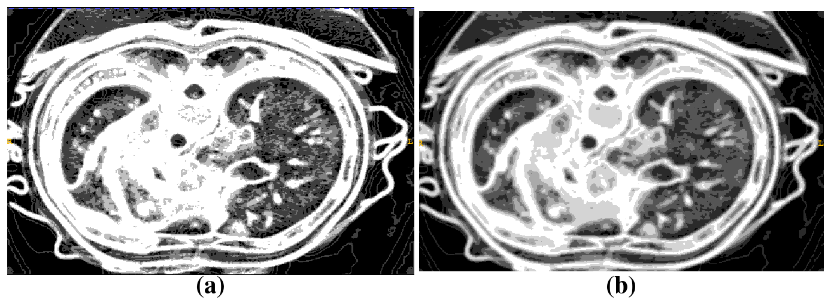
Figure 1. Entropy computed for two different neighborhood sizes: (a) 3 × 3 × 3 voxels and (b) 5 × 5 × 5 voxels.
Computation 04 00035 g001
Figure 2. Binary masks obtained from the results of entropy computation: (a) 3 × 3 × 3 voxels and (b) 5 × 5 × 5 voxels.
Computation 04 00035 g002
Figure 3. Segmentation of the lipid droplet. (a) sharp image slice and (b) its noisy thresholding result; (c) blurred slice; and (d) its thresholding result.
Computation 04 00035 g003
Figure 4. Intensity histogram (black line) of the cropped FIB dataset containing inhomogeneous lipid droplet; The red line shows the threshold for inhomogeneous inclusions; the blue line—the threshold of lipid droplet.
Computation 04 00035 g004
Figure 5. Results of spleen segmentation: α = 0.2 , β = 0.95 .
Computation 04 00035 g005
Figure 6. Results of liver segmentation: α = 0.2 , β = 0.95 .
Computation 04 00035 g006
Figure 7. Segmentation errors near aorta border: (a) coronary arteries may be either connected or disconnected with segmentation “leaks”; (b) errors near ostia points show that false vesselness filter response may be both inside and outside of the aorta; (c) errors in the cerebral case and (d) result of our algorithm application. Green—aorta, red—mask of coronary vessels, purple—mask of cerebral vessels.
Computation 04 00035 g007
Figure 8. Results of cerebral arteries segmentation: (a,b) resulting segmentations, green—aorta, purple—cerebral arteries.
Computation 04 00035 g008
Figure 9. 3D volume reconstruction of a lipid droplet. (a) internal structure of lipid droplet; (b) whole structure.
Computation 04 00035 g009
Table 1. Results of entropy feature computation for two Computed Tomography (CT) datasets: image dimensions and computation times for both Central Processing Unit (CPU) and Graphics Processing Unit (GPU) version of the program code.
Dataset Size, VoxelsCPU Time, sGPU Time, s
512 × 335 × 200 735139
430 × 346 × 277 1189198
Table 2. CPU times of cerebral arteries segmentation.
DatasetDataset 1Dataset 2
Resolution 512 × 512 × 501 512 × 512 × 451
Spacing 0 . 76 × 0 . 76 × 0 . 80 mm 0 . 62 × 0 . 62 × 0 . 80 mm
Pulmonary removal 7 . 76 s 7 . 04 s
Aorta segmentation 16 . 61 s 15 . 33 s
Frangi Vesselness 196 . 40 s 184 . 91 s
Aortic arch branches 7 . 61 s 6 . 67 s
Aorta border cleaning 7 . 39 s 6 . 76 s