Modeling Groundwater Flow in Heterogeneous Porous Media with YAGMod

Abstract

Modeling flow and transport in porous media requires the management of complexities related both to physical processes and to subsurface heterogeneity. A thorough approach needs a great number of spatially-distributed phenomenological parameters, which are seldom measured in the field. For instance, modeling a phreatic aquifer under high water extraction rates is very challenging, because it requires the simulation of variably-saturated flow. 3D steady groundwater flow is modeled with YAGMod (yet another groundwater flow model), a model based on a finite-difference conservative scheme and implemented in a computer code developed in Fortran90. YAGMod simulates also the presence of partially-saturated or dry cells. The proposed algorithm and other alternative methods developed to manage dry cells in the case of depleted aquifers are analyzed and compared to a simple test. Different approaches yield different solutions, among which, it is not possible to select the best one on the basis of physical arguments. A possible advantage of YAGMod is that no additional non-physical parameter is needed to overcome the numerical difficulties arising to handle drained cells. YAGMod also includes a module that allows one to identify the conductivity field for a phreatic aquifer by solving an inverse problem with the comparison model method.

1. Introduction

The flow of water in porous sediments is described in mathematical terms by joining the mass conservation principle with the phenomenological Darcy’s law [1,2]. This results in non-linear equations for variably-saturated media and linear equations for fully-saturated ones. Non-linearity in the forward problem, which is solved to predict the state of the system in response to some forcing (e.g., pumping rates), is introduced by source terms or boundary conditions. The forward problem can be solved analytically only for simple cases, i.e., usually for homogeneous media, domains with simple geometries and for simple source terms. Therefore, analytical solutions can be useful to interpret the results of field tests, e.g., pumping and tracer tests, and of laboratory experiments, where the boundary conditions can be effectively controlled. On the other hand, their use to predict the behavior of complex natural systems is limited by the assumptions that are introduced to simplify the equations and the boundary conditions. Therefore, in practical applications, a variety of computer codes, based on the classical numerical methods of the solution of partial differential equations (finite differences, finite elements, finite volumes, etc.), is used to solve the forward problem.

One of the most challenging problems in hydrogeology is modeling variably-saturated groundwater flow processes. A fully-rigorous solution of this problem requires knowledge of the non-linear relationship of conductivity and matric potential with soil water content, for all the lithologies recognized in the subsoil. Therefore, approximated approaches, which introduce relatively simple modifications of the classical equations for saturated groundwater flow, are often applied. They give rise to numerical difficulties in the presence of dry cells or elements, e.g., under the influence of an extraction source term. When a cell becomes dry, i.e., its calculated water level falls below the bottom of the cell, two main problems arise [3,4,5,6]. First, the dry cell cannot receive external water, if it is declared as “inactive”; neither can it contain any extraction source term, unless it is rewetted, i.e., the water level rises above a prescribed threshold. Second, drying and rewetting functionality often yields difficulties for the convergence of iterative algorithms used for the solution of the algebraic equations of the discrete model. Doherty [3] proposes an asymptotically small transmissivity to avoid drained cells being deactivated, even if they actually become dry: this approach uses a function that prevents cell transmissivity from becoming negative. The innovative idea of Keating and Zyvoloski [4] is a weak scaling for vertical connectivity, from partially-saturated to dry conditions. On the other hand, Niswonger et al. [6] use a quadratic approximation of the function that relates horizontal conductance to hydraulic head, over small intervals close to the fully-dry and fully-saturated limits.

Within this background, the first goal of this paper is to propose a code, YAGMod (yet another groundwater flow model), developed in Fortran90, for the simulation of constant-density, groundwater flow under stationary conditions, which is the extension of the codes developed by our research team over the years [7,8,9,10,11,12,13,14,15,16,17]. YAGMod is based on a conservative finite difference scheme for stationary conditions and is oriented to the simulation of flow in saturated media. It takes into account the possible drying of shallow blocks of the domain with an original approach, which limits the number of additional parameters that have to be assigned by the user and that have a weak physical significance. Notice that YAGMod considers both prescribed distributed sources and variable point sources. While the former can be used to simulate aquifer recharge, the latter can be used to simulate draining systems or the effects of the water head drawdown on a water-well discharge.

The second goal of this paper is to compare the algorithm used by YAGMod to handle desaturated cells with the above-mentioned algorithms proposed by Doherty [3], Keating and Zyvoloski [4] and Niswonger et al. [6]. This is performed by means of a simple, but significant test case.

Moreover, YAGMod includes a module for the model calibration, namely the identification of transmissivity from the knowledge of the reference head and source fields all over the domain. The calibration is performed for 2D flow conditions implementing the comparison model method (CMM). This method was originally proposed by Scarascia and Ponzini [18], successively developed by Ponzini and Lozej [19] and cast in a more formal mathematical framework by Ponzini and Crosta [20]. The CMM has been applied and implemented with success to study 2D hydraulic flow in regional aquifers [14,16,17,21,22,23], and therefore, for the moment, its implementation within YAGMod covers these kinds of systems only.

The third goal of this paper is a thorough and rigorous extension of the CMM to the case of a phreatic aquifer. This is possible because YAGMod takes into account the variation of the saturated thickness of each cell for the solution of the forward problem.

Generally speaking, the “best” model should permit one to properly describe the physical processes and should run with limited computational resources. Unfortunately, these objectives are usually conflicting: physical processes in natural systems might be very complex, non-linear and dependent on a huge number of physical parameters; the computer codes that can handle such situations require supercomputers with high memory capacity and a lot of parallel processors. Simplified approaches are commonly adopted by scientists and engineers. Nevertheless, relatively simple models and tests, like those proposed in this paper, can be very useful to cope with complex natural systems with a computationally-frugal approach, which can provide first insights into the relevant natural processes, on the most sensitive parameters, etc., as recently shown, e.g., by Hill et al. [24].

2. Forward Model

This section is dedicated to a description of YAGMod, and particular emphasis will be given to its innovative features.

2.1. Mathematical Model and Discretization

The 3D flow of groundwater, considering constant fluid density and steady-state conditions, is described by the balance equation:

$$div\mathbf{q}=f$$

(1)

which, using the phenomenological Darcy’s law $\mathbf{q}=-K\mathbf{grad}h$, becomes:

$$\frac{\partial }{\partial x}\left(K\frac{\partial h}{\partial x}\right)+\frac{\partial }{\partial y}\left(K\frac{\partial h}{\partial y}\right)+\frac{\partial }{\partial z}\left(K\frac{\partial h}{\partial z}\right)+f=0$$

(2)

where $\mathbf{q}$ is Darcy’s velocity ($\mathrm{L}{\mathrm{T}}^{-1}$); h is the water or hydraulic head (L); f is the source term, i.e., the volume of water injected per unit time and unit volume of the porous medium (${\mathrm{T}}^{-1}$); K is the hydraulic conductivity ($\mathrm{L}{\mathrm{T}}^{-1}$).

The numerical solution of Equation (2) is found with the finite difference method. The continuous physical system is replaced by a finite set of cells or blocks, which are identified by three integer indices $(i,j,k)$, $1\le i\le N_x$, $1\le j\le N_z$ and $1\le k\le N_z$, and could be rectangular in the horizontal plane. The side lengths of the cells along the x and y directions, $\Delta x$ and $\Delta y$, are assumed to be constant for all of the grid; the cell thickness, denoted by $\Delta z_{(i,j,k)}$, can vary for each cell. The center of a cell is called a node and is denoted with the same indices as the corresponding cell. Values of the hydraulic head are referred to each node, and the spatially-varying hydraulic conductivities are considered to be effective parameters of a cell.

The saturated thickness of a cell is given by:

$${\vartheta }_{(i,j,k)}=\left\{\begin{array}{cc}\Delta z_{(i,j,k)}=z_{(i,j,k)}^{\left(\mathrm{top}\right)}-z_{(i,j,k)}^{\left(\mathrm{bot}\right)}\hfill & \mathrm{if}{h}_{(i,j,k)}>z_{(i,j,k)}^{\left(\mathrm{top}\right)},\hfill \\ h_{(i,j,k)}-z_{(i,j,k)}^{\left(\mathrm{bot}\right)}\hfill & \mathrm{if}{z}_{(i,j,k)}^{\left(\mathrm{bot}\right)}<h_{(i,j,k)}\le z_{(i,j,k)}^{\left(\mathrm{top}\right)},\hfill \\ 0\hfill & \mathrm{if}{h}_{(i,j,k)}\le z_{(i,j,k)}^{\left(\mathrm{bot}\right)}\hfill \end{array}\right.$$

(3)

where $z_{(i,j,k)}^{\left(\mathrm{top}\right)}$ and $z_{(i,j,k)}^{\left(\mathrm{bot}\right)}$ represent the height of, respectively, the top and bottom surfaces of a cell.

For each cell, an integral balance equation can be written. The water discharge into or from a cell is calculated considering only the six adjacent (first-neighborhood) cells (Figure 1).

In order to handle complex aquifers’ geometries, each cell is identified by a domain code (Figure 2): I identifies the internal cells, for which the hydraulic head can vary freely; D identifies the cells where Dirichlet conditions are assigned, i.e., the hydraulic head is prescribed; E identifies the cells external to the domain or where no flow takes place.

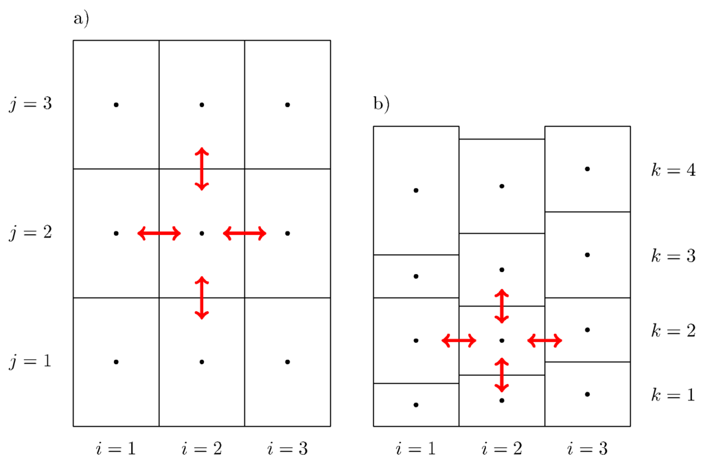
Figure 1. (a) Plan view of a domain’s layer; (b) vertical section view. Red arrows are examples of groundwater fluxes through first-neighborhood cells and considered in the discrete model.

Figure 1. (a) Plan view of a domain’s layer; (b) vertical section view. Red arrows are examples of groundwater fluxes through first-neighborhood cells and considered in the discrete model.

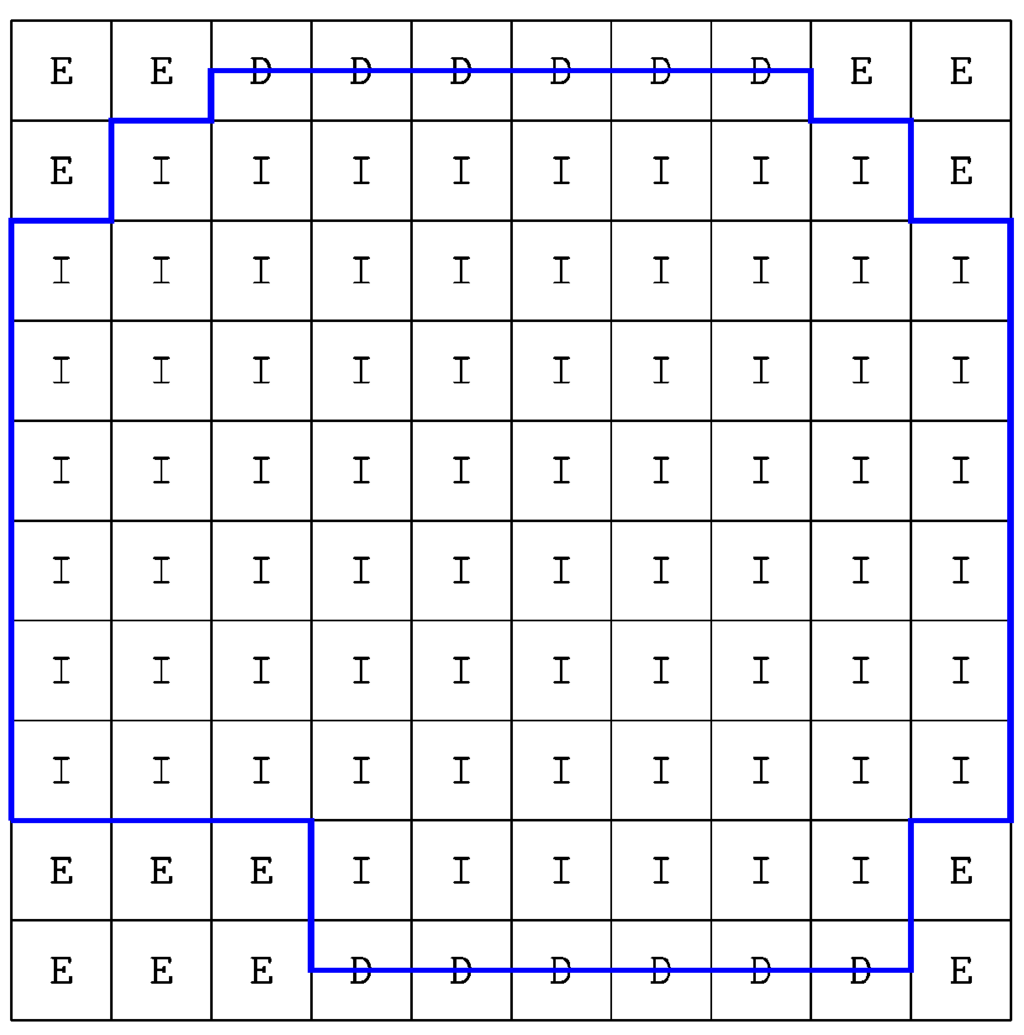
Figure 2. Domain code example in a 2D domain: I, E and D codes correspond, respectively, to internal, external and prescribed-head (Dirichlet boundary conditions) cells; the blue line denotes the border of the domain.

Figure 2. Domain code example in a 2D domain: I, E and D codes correspond, respectively, to internal, external and prescribed-head (Dirichlet boundary conditions) cells; the blue line denotes the border of the domain.

The integral version of Equation (2) could be discretized for each cell as:

$$\begin{array}{ccc}\hfill {\displaystyle K_{(i+1/2,j,k)}\frac{h_{(i+1,j,k)}-h_{(i,j,k)}}{\Delta x}\Delta y{\vartheta }_{(i+1/2,j,k)}}& +& \hfill \\ \hfill \\ \hfill {\displaystyle +K_{(i-1/2,j,k)}\frac{h_{(i-1,j,k)}-h_{(i,j,k)}}{\Delta x}\Delta y{\vartheta }_{(i-1/2,j,k)}}& +& \hfill \\ \hfill \\ \hfill {\displaystyle +K_{(i,j+1/2,k)}\frac{h_{(i,j+1,k)}-h_{(i,j,k)}}{\Delta y}\Delta x{\vartheta }_{(i,j+1/2,k)}}& +& \hfill \\ \hfill \\ \hfill {\displaystyle +K_{(i,j-1/2,k)}\frac{h_{(i,j-1,k)}-h_{(i,j,k)}}{\Delta y}\Delta x{\vartheta }_{(i,j-1/2,k)}}& +& \hfill \\ \hfill \\ \hfill {\displaystyle +K_{(i,j,k+1/2)}\frac{h_{(i,j,k+1)}-h_{(i,j,k)}}{\Delta z_{(i,j,k+1/2)}}\Delta x\Delta y}& +& \hfill \\ \hfill \\ \hfill {\displaystyle +K_{(i,j,k-1/2)}\frac{h_{(i,j,k-1)}-h_{(i,j,k)}}{\Delta z_{(i,j,k-1/2)}}\Delta x\Delta y}& +& F_{(i,j,k)}=0\hfill \end{array}$$

where $h_{(i,j,k)}$ is the hydraulic head at a node (L); $K_{(i-1/2,j,k)}$ and $K_{(i+1/2,j,k)}$ (${\mathrm{LT}}^{-1}$) are called internode (or interblock) hydraulic conductivities along the x direction (analogous definitions are used for the similar terms along the y and z directions); ${\vartheta }_{(i+1/2,j,k)}=\left({\vartheta }_{(i,j,k)}+{\vartheta }_{(i+1,j,k)}\right)/2$ is the arithmetic mean of the saturated thicknesses of the cells $(i,j,k)$ and $(i+1,j,k)$ (an analogous definition is used for cells along the y direction); $\Delta z_{(i,j,k+1/2)}=\left(\Delta z_{(i,j,k)}+\Delta z_{(i+1,j,k)}\right)/2$ is the distance between two adjacent nodes along the vertical; $F_{(i,j,k)}$ is the cell source term, i.e., the volume of water injected in the cell (negative if extracted from) per unit time (${\mathrm{L}}^3{\mathrm{T}}^{-1}$). Each of the nine terms appearing in the left-hand side of Equation (4) represents the water flux through an interface separating two cells.

A single value of hydraulic conductivity is assigned to every cell, and the internode hydraulic conductivity is calculated as the harmonic mean of the hydraulic conductivities of adjacent cells.

Equation (4) can be synthetically written for the most general case, by introducing internode transmittances as follows:

$$\begin{array}{ccc}\hfill {\mathcal{T}}_{(i+1/2,j,k)}& =& {\displaystyle K_{(i+1/2,j,k)}{\vartheta }_{(i+1/2,j,k)}\frac{\Delta y}{\Delta x},}\hfill \\ \\ \hfill {\mathcal{T}}_{(i,j+1/2,k)}& =& {\displaystyle K_{(i,j+1/2,k)}{\vartheta }_{(i,j+1/2,k)}\frac{\Delta x}{\Delta y},}\hfill \\ \\ \hfill {\mathcal{T}}_{(i,j,k+1/2)}& =& {\displaystyle K_{(i,j,k+1/2)}\frac{\Delta x\Delta y}{\Delta z_{(i,j,k+1/2)}}}\hfill \end{array}$$

(4)

Then, Equation (4) becomes:

$$\begin{array}{ccccc}& {\mathcal{T}}_{(i+1/2,j,k)}\left(h_{(i+1,j,k)}-h_{(i,j,k)}\right)\hfill & +& {\mathcal{T}}_{(i-1/2,j,k)}\left(h_{(i-1,j,k)}-h_{(i,j,k)}\right)\hfill & +\\ \hfill +& {\mathcal{T}}_{(i,j+1/2,k)}\left(h_{(i,j+1,k)}-h_{(i,j,k)}\right)\hfill & +& {\mathcal{T}}_{(i,j-1/2,k)}\left(h_{(i,j-1,k)}-h_{(i,j,k)}\right)\hfill & +\\ \hfill +& {\mathcal{T}}_{(i,j,k+1/2)}\left(h_{(i,j,k+1)}-h_{(i,j,k)}\right)\hfill & +& {\mathcal{T}}_{(i,j,k-1/2)}\left(h_{(i,j,k-1)}-h_{(i,j,k)}\right)\hfill & =\\ \hfill =& -F_{(i,j,k)}\hfill \end{array}$$

(5)

2.2. Boundary Conditions and Source Terms

Dirichlet, Neumann or Robin boundary conditions can be assigned. The cells where Dirichlet boundary conditions (prescribed head) are assigned are simply identified by using a D label for the domain code: in that case, the hydraulic head does not change during the computation of the solution. Neumann and Robin boundary conditions are implemented as specific types of source terms, as specified hereinafter.

2.2.1. Distributed Source/Sink Terms

This type of source or sink term simulates areally-distributed fixed source terms, such as rainfall recharge. For each contribution, an array of $N_x\times N_y\times N_z$ elements, $F_{(i,j,k)}^{\left(\text{d}\right)}$, represents the flow rate into each cell of the domain; it is independent from $h_{(i,j,k)}$, and its dimensions are (${\mathrm{L}}^3{\mathrm{T}}^{-1}$). The user must consider that this type of source remains constant, even if the hydraulic head of a single cell becomes lower than the bottom of the cell during the iterative search of a solution.

2.2.2. Local Source/Sink Terms

In the YAGMod code, local sources or sinks, i.e., those that are concentrated in a single cell, are modeled with the paradigmatic equation:

$$\begin{array}{cc}{F}^{\left(\mathrm{loc}\right)}=\hfill & \left\{\begin{array}{cc}{F}_{(+)}-{\mathcal{K}}_{(+)}·(h-{\mathcal{H}}^{\left(\mathrm{cal}\right)})\hfill & \mathrm{if}h\ge {\mathcal{H}}^{\left(\mathrm{act}\right)},\hfill \\ F_{(-)}-{\mathcal{K}}_{(-)}·(h-{\mathcal{H}}^{\left(\mathrm{cal}\right)})\hfill & \mathrm{if}h<{\mathcal{H}}^{\left(\mathrm{act}\right)}\hfill \end{array}\right.\hfill \end{array}$$

(6)

where $F^{\left(\mathrm{loc}\right)}$ is the local contribution of the individual source or sink. $F^{\left(\mathrm{loc}\right)}$ depends on the hydraulic head in that cell, h, according to the difference $(h-{\mathcal{H}}^{\left(\mathrm{cal}\right)})$. $F_{(+)}$ and $F_{(-)}$ are fixed fluxes (${\mathrm{L}}^3{\mathrm{T}}^{-1}$); ${\mathcal{K}}_{(+)}$ and ${\mathcal{K}}_{(-)}$ are conductances (${\mathrm{L}}^2{\mathrm{T}}^{-1}$); ${\mathcal{H}}^{\left(\mathrm{cal}\right)}$ and ${\mathcal{H}}^{\left(\mathrm{act}\right)}$ are two reference head values (L). ${\mathcal{H}}^{\left(\mathrm{act}\right)}$ is a threshold, which establishes if a source or sink is active or which couple of fluxes and conductances, $(F_{(+)},{\mathcal{K}}_{(+)})$ or $(F_{(-)},{\mathcal{K}}_{(-)})$, should be used to compute $F^{\left(\mathrm{loc}\right)}$; ${\mathcal{H}}^{\left(\mathrm{cal}\right)}$, which could be equal to ${\mathcal{H}}^{\left(\mathrm{act}\right)}$ in many cases, is used to calculate the contribution to the source term, which linearly depends on h. All of these parameters can be separately defined for each source or sink.

Different combinations of $F_{(+)}$, $F_{(-)}$, ${\mathcal{K}}_{(+)}$, ${\mathcal{K}}_{(-)}$, ${\mathcal{H}}^{\left(\mathrm{act}\right)}$ and ${\mathcal{H}}^{\left(\mathrm{cal}\right)}$ allow the user to generate a great variety of source terms, some of which are listed and briefly described below.

• Drain:
  $F_{(+)}=F_{(-)}=0$, ${\mathcal{K}}_{(-)}=0$; ${\mathcal{K}}_{(+)}$ represents the drain conductance; ${\mathcal{H}}^{\left(\mathrm{act}\right)}={\mathcal{H}}^{\left(\mathrm{cal}\right)}$ represents the drain elevation.
• Robin boundary conditions:
  These conditions can be used if the aquifer interacts with another water body and water exchange is controlled by the difference of the water head in the aquifer and in the external water body. They are introduced through Equation (6), by assigning the following parameters: $F_{(+)}=F_{(-)}=0$; ${\mathcal{H}}^{\left(\mathrm{act}\right)}={\mathcal{H}}^{\left(\mathrm{cal}\right)}$ are the reference hydraulic heads; ${\mathcal{K}}_{(+)}$ and ${\mathcal{K}}_{(-)}$ represent the conductances for flux out or into the cell. ${\mathcal{K}}_{(+)}$ and ${\mathcal{K}}_{(-)}$ depend on the conductivity of the materials that separate the aquifer from the water body at the reference water head and on the distance from this water body. Notice that for the simulation of limited domains of aquifers with a large extension, it is usually impossible to prescribe physically-based boundary conditions. In those cases, Robin boundary conditions are very useful to introduce fictitious boundary conditions, which are more flexible than prescribed head (Dirichlet) or flux (Neumann) boundary conditions. In these situations, ${\mathcal{H}}^{\left(\mathrm{act}\right)}={\mathcal{H}}^{\left(\mathrm{cal}\right)}$ should be close to the estimated water head far from the aquifer system, and the conductances ${\mathcal{K}}_{(+)}$ and ${\mathcal{K}}_{(-)}$ can assume different values to take into account the geometrical, geological and hydrological characteristics of the aquifer.
• River/aquifer interaction:
  ${\mathcal{H}}^{\left(\mathrm{act}\right)}$ is the height of the bottom of the river: therefore, if $h\ge {\mathcal{H}}^{\left(\mathrm{act}\right)}$, the river and groundwater are in contact, whereas, if $h<{\mathcal{H}}^{\left(\mathrm{act}\right)}$, then they are separated by a vadose zone, i.e., partly-saturated sediments or rocks. In the first situation, ${\mathcal{H}}^{\left(\mathrm{cal}\right)}$ is the river stage; then, the river drains the aquifer if $h>{\mathcal{H}}^{\left(\mathrm{cal}\right)}$ and recharges the aquifer if $h<{\mathcal{H}}^{\left(\mathrm{cal}\right)}$. It is quite common to assume $F_{(+)}=0$ and to consider ${\mathcal{K}}_{(+)}$ as a function of the conductivity of the river bed sediments, their thickness and the area of the contact surface between the river bed and the aquifer in the considered cell. In the second situation, namely if $h<{\mathcal{H}}^{\left(act\right)}$, the river bed is assumed to be composed of fine-grained materials, which could be almost saturated, but poorly permeable, whereas the vadose zone between the river bed and the water table could be more permeable than the river bed sediments and approximated as dry. Therefore, the water flows through the river bed under a gravity-controlled, unit hydraulic gradient and freely flows through the relatively permeable vadose zone: then, ${\mathcal{K}}_{(-)}=0$, whereas $F_{(-)}$ depends on the conductivity, thickness and extension of the river bed sediments in the considered cell and on the river stage.

2.2.3. Screened Wells

YAGMod considers a new kind of source term that takes into account the dependence of the wells’ extraction rate on the aquifer water head. In particular, this kind of source term allows one to turn off the pumping if a cell becomes dry. Sources in this category are denoted as “screened wells”, as the user has to give as input data not only the $(x,y)$ coordinates of the well, i.e., the node indices $i_W$ and $j_W$, but also the top and bottom elevation of the screened interval ($to{p}_{\mathrm{W}}$ and $bo{t}_{\mathrm{W}}$) and the maximum well extraction rate, $q_w$.

The maximum extraction rate is subdivided among the cells intersected by screened intervals, as:

$$q_{(i_W,j_W,k)}^{\left(\mathrm{scr}\right)}=q_W·\frac{K_{(i_W,j_W,k)}{\mathcal{L}}_{(i_W,j_W,k)}^{\left(\mathrm{scr}\right)}}{{\sum }_{k^{\prime }=n^{\left(\min \right)}}^{n^{\left(\max \right)}}{K}_{(i_W,j_W,k^{\prime })}{\mathcal{L}}_{(i_W,j_W,k^{\prime })}^{\left(\mathrm{scr}\right)}}$$

(7)

with $k=n^{\left(\min \right)},\dots ,n^{\left(\max \right)}$, where: $n^{\left(\min \right)}$ and $n^{\left(\max \right)}$ are the indices (along the vertical direction) of the cells corresponding to the top and the bottom of the screened interval of the well; ${\mathcal{L}}_{(i_W,j_W,k)}^{\left(\mathrm{scr}\right)}$ is the screened thickness of the well corresponding to a fully-saturated porous medium within the $(i_W,j_W,k)$ cell and is computed as:

$${\mathcal{L}}_{(i_W,j_W,k)}^{\left(\mathrm{scr}\right)}=min\left(h_{(i_W,j_W,k)},s_{(i_W,j_W,k)}^{\left(\mathrm{top}\right)}\right)-min\left(h_{(i_W,j_W,k)},s_{(i_W,j_W,k)}^{\left(\mathrm{bot}\right)}\right)$$

(8)

where:

$$s_{(i_W,j_W,k)}^{\left(\mathrm{top}\right)}=\left\{\begin{array}{cc}{z}_{(i_W,j_W,k)}^{\left(\mathrm{top}\right)}\hfill & k=n^{\left(\min \right)},\dots ,n^{\left(\max \right)}-1,\hfill \\ to{p}_{\mathrm{W}}\hfill & k=n^{\left(\max \right)}\hfill \end{array}\right.$$

(9)

and:

$$s_{(i_W,j_W,k)}^{\left(\mathrm{bot}\right)}=\left\{\begin{array}{cc}{z}_{(i_W,j_W,k)}^{\left(\mathrm{bot}\right)}\hfill & k=n^{\left(\min \right)}+1,\dots ,n^{\left(\max \right)},\hfill \\ bo{t}_{\mathrm{W}}\hfill & k=n^{\left(\min \right)}\hfill \end{array}\right.$$

(10)

Notice that if $h_{(i_W,j_W,k)}<s_{(i_W,j_W,k)}^{\left(\mathrm{bot}\right)}$, then ${\mathcal{L}}_{(i_W,j_W,k)}^{\left(\mathrm{scr}\right)}=0$.

If the cell $(i_W,j_W,k)$ desaturates, the value of $q_{(i_W,j_W,k)}^{\left(scr\right)}$ is corrected, so that the contribution of the well to the source term of the cell $(i_W,j_W,k)$ is given by:

$$F_{(i_W,j_W,k)}^{\left(\mathrm{s}\right)}=q_{(i_W,j_W,k)}^{\left(\mathrm{scr}\right)}·\frac{\sqrt{{\mathcal{L}}_{(i_W,j_W,k)}^{\left(\mathrm{scr}\right)}}}{s_{(i_W,j_W,k)}^{\left(\mathrm{top}\right)}-s_{(i_W,j_W,k)}^{\left(\mathrm{bot}\right)}}$$

(11)

The latter equation implies that, at a given location, the water extracted from a cell reduces as the square root of the thickness of the screened interval that intersects a fully-saturated portion of the aquifer in that cell.

2.3. Solution of the Balance Equations

Equation (5) can be written for each internal cell, resulting in a system of possibly non-linear equations that can be written in matrix formulation as:

$$\mathbf{A}\left(\mathbf{x}\right)\mathbf{x}={\mathbf{b}}^{\left(\mathrm{fix}\right)}+{\mathbf{b}}^{\left(\mathrm{var}\right)}\left(\mathbf{x}\right)$$

(12)

where $\mathbf{x}$ includes the values of the water head in the internal nodes, ${\mathbf{b}}^{\left(\mathrm{fix}\right)}$ includes the fixed source/sink terms (Section 2.2.1), ${\mathbf{b}}^{\left(\mathrm{var}\right)}$ includes the source/sink terms that depend on the water head of the aquifer (Section 2.2.2 and Section 2.2.3) and the terms appearing in the left-hand side of Equation (5) that involve the water head at D nodes. $\mathbf{A}$ is a sparse, symmetric, diagonally-dominant matrix, which is strictly diagonally dominant if at least one D node is present in the domain; its elements are built with transmittances and, therefore, depend on $\mathbf{x}$, as shown by Equations (3) and (4).

The solution to Equation (12) could be obtained with any of the methods of solution for non-linear equations that can be found in textbooks of numerical analysis. In YAGMod, a simple approach, based on a generalization of the relaxation methods for the solution of systems of algebraic linear equations, is proposed. This choice is optimal from the point of view of the memory requirement. Other approaches, e.g., Newton’s or conjugate-gradient methods, could be more efficient in terms of elapsed running time, if the code is properly modified to profit from parallel computers. However, it should be noted that the specific problem addressed in this paper includes non-differentiable terms in the system of equations, like those introduced by Equation (6) and by the sequence of equations from Equations (7) to (11). Several tests showed that the generalization of relaxation methods is in general quite robust, in particular for complex physical situations.

2.4. Check of the Physical Consistency of the Solution

The proposed model does not solve equations for variably-saturated conditions, but aims at finding a solution for fully-saturated groundwater flow: the cells that become dry during the iterative algorithm of solution are not eliminated from the domain, but are used as auxiliary cells in the sense to be specified below.

If $h_{(i+1,j,k)}<z_{(i+1,j,k)}^{\left(\mathrm{bot}\right)}$, then ${\vartheta }_{(i+1,j,k)}=0$. If also the adjacent cells along the horizontal directions are dry, then the terms corresponding to horizontal fluxes in Equation (5) vanish, and therefore, the cell under examination is involved only for a balance along the vertical direction. This choice permits one to transfer the fixed source terms to deeper cells: this is necessary, e.g., to permit the aquifer recharge, which is assigned at the top active (i.e., internal) cells, to reach the water table. Instead, if the adjacent cells have a non-vanishing, possibly small, thickness, then the physical situation implies that there is a horizontal transfer of water.

When the solution procedure is completed (Section 2.3), the computer code checks the physical reliability of the solution reached. First, a recursive function searches for every continuous path connecting partially- or totally-desaturated cells with the uppermost active cells. At the end of this checking step, every totally- or partially-desaturated cell needs to be connected with the surface, in order to allow air to infiltrate into the porous medium. Second, another function searches for the totally-desaturated cells for which the sum of all of the source terms is negative: such cells actually contain some outflowing source terms, but extracting water from a dry cell cannot be physically acceptable.

If one of these two physically unacceptable conditions occur (desaturated cells not connected with the surface; net outflowing source term from dry cells), YAGMod prints a warning message to the standard output and in the summary output file.

2.5. An Example

To show the relevance of these checks and the behavior of the code when dealing with screened wells, two simulations have been run using two different ways to manage an extraction source term. The domain is built up with $100\times 100\times 28$ cells of $2.5\mathrm{m}\times 2.5\mathrm{m}\times 2.5\mathrm{m}$ dimensions. A low conductivity lens ($K^{\left(\mathrm{L}\right)}={10}^{-8}\mathrm{m}/\mathrm{s}$) is included in a homogeneous, permeable medium ($K^{\left(\mathrm{H}\right)}={10}^{-4}\mathrm{m}/\mathrm{s}$). In the first simulation, a single deep well, whose extraction rate is about $0.06{\mathrm{m}}^3/\mathrm{s}$, is located beneath the lens at $\mathrm{x}=125\mathrm{m}$ and $\mathrm{z}=20\mathrm{m}$; in the second one, the single deep well is replaced by a screened well, from $20\mathrm{m}$ to $45\mathrm{m}$, whose extraction rate is the same as the other (obviously, distributed along the whole screened interval). In the latter case, the extraction rate is controlled by the hydraulic head. Results are shown in Figure 3. The simulation run with the deep fixed extraction rate yields physically inconsistent results: in fact, a group of completely desaturated cells is not connected with the surface. On the other hand, the simulation run with the screened well leads to a physically acceptable solution.

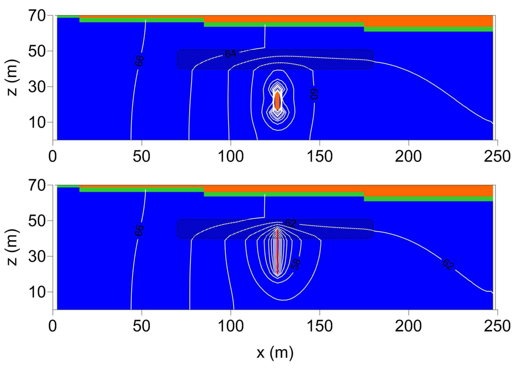
Figure 3. Contour lines of the hydraulic head (2-meter contour interval) and map of the saturation field (fully-saturated cells are drawn in blue; partially-saturated cells are drawn in green; dry cells are drawn in orange) along a vertical section for a 3D problem solved with YAGMod (yet another groundwater flow model). (top) A single deep well, whose fixed extraction rate is about $0.06{\mathrm{m}}^3/s$, is located at $x=125\mathrm{m}$ and $z=20\mathrm{m}$, beneath a low conductivity lens (dashed area). (bottom) The single deep well is replaced by a screened well, from $20\mathrm{m}$ to $45\mathrm{m}$ (yellow line).

Figure 3. Contour lines of the hydraulic head (2-meter contour interval) and map of the saturation field (fully-saturated cells are drawn in blue; partially-saturated cells are drawn in green; dry cells are drawn in orange) along a vertical section for a 3D problem solved with YAGMod (yet another groundwater flow model). (top) A single deep well, whose fixed extraction rate is about $0.06{\mathrm{m}}^3/s$, is located at $x=125\mathrm{m}$ and $z=20\mathrm{m}$, beneath a low conductivity lens (dashed area). (bottom) The single deep well is replaced by a screened well, from $20\mathrm{m}$ to $45\mathrm{m}$ (yellow line).

3. A Simple Test Case to Compare Different Approaches to Handle Dry Cells

A number of different approaches to manage dry cells has been proposed [3,4,6]. Each approach calculates internode conductivities in a different way; in some cases, also effective extraction rates are calculated taking into account the saturated thickness. In this section, the algorithm implemented in YAGMod is compared to those approaches by means of a test case, which is very simple, but permits one to emphasize some significant properties of the different methods. In particular, the basic characteristics of the analyzed algorithms are briefly recalled using a simplified notation based on this example. A simple 2D domain has been constructed with a grid of $3\times 1\times 2$ cells whose size is $100\mathrm{m}\times 100\mathrm{m}\times 20\mathrm{m}$. This 2D domain is illustrated in Figure 4, together with the cell numbering used in the following for the sake of simplicity.

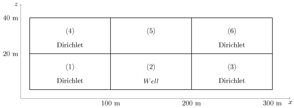
Figure 4. Scheme of the 2D domain used for the comparison test.

Figure 4. Scheme of the 2D domain used for the comparison test.

At cells $\left(1\right)$, $\left(3\right)$, $\left(4\right)$ and $\left(6\right)$, the hydraulic head is prescribed in such a way as to generate a hydraulic gradient along the x direction: $h_{\left(1\right)}=h_{\left(4\right)}=40\mathrm{m}$, $h_{\left(3\right)}=h_{\left(6\right)}=39\mathrm{m}$. At cell $\left(2\right)$, an extraction source term is assigned.

The balance equations for the internal cells (2) and (5) can be written as:

$$\begin{array}{cccc}& \hfill {\displaystyle K_{(1,2)}{\vartheta }_{(1,2)}\frac{h_{\left(1\right)}-h_{\left(2\right)}}{\Delta x}\Delta y}& +& \\ \\ \hfill +& \hfill {\displaystyle K_{(3,2)}{\vartheta }_{(3,2)}\frac{h_{\left(3\right)}-h_{\left(2\right)}}{\Delta x}\Delta y}& +& \\ \\ \hfill +& \hfill {\displaystyle K_{(5,2)}\frac{h_{\left(5\right)}-h_{\left(2\right)}}{\Delta z}\Delta x\Delta y}& =& -F_{\left(2\right)}\hfill \end{array}$$

(13)

and:

$$\begin{array}{cccc}& \hfill {\displaystyle K_{(4,5)}{\vartheta }_{(4,5)}\frac{h_{\left(4\right)}-h_{\left(5\right)}}{\Delta x}\Delta y}& +& \\ \\ \hfill +& \hfill {\displaystyle K_{(6,5)}{\vartheta }_{(6,5)}\frac{h_{\left(6\right)}-h_{\left(5\right)}}{\Delta x}\Delta y}& +& \\ \\ \hfill +& \hfill {\displaystyle K_{(2,5)}\frac{h_{\left(2\right)}-h_{\left(5\right)}}{\Delta z}\Delta x\Delta y}& =& 0\hfill \end{array}$$

(14)

In the numerical experiments conducted in this work, $h_{\left(2\right)}$ and $h_{\left(5\right)}$ vary from minimum to maximum values, i.e., in the interval from 0 m to 40 m. The balance errors ${ϵ}_{\left(2\right)}$ and ${ϵ}_{\left(5\right)}$ are calculated as:

$$\begin{array}{ccccc}\hfill {ϵ}_{\left(2\right)}& =& {\displaystyle K_{(1,2)}{\vartheta }_{(1,2)}\frac{h_{\left(1\right)}-h_{\left(2\right)}}{\Delta x}\Delta y}\hfill & +& \\ \\ & +& {\displaystyle K_{(3,2)}{\vartheta }_{(3,2)}\frac{h_{\left(3\right)}-h_{\left(2\right)}}{\Delta x}\Delta y}\hfill & +& \\ \\ & +& {\displaystyle K_{(5,2)}\frac{h_{\left(5\right)}-h_{\left(2\right)}}{\Delta z}\Delta x\Delta y}\hfill & +& F_{\left(2\right)}\hfill \end{array}$$

(15)

$$\begin{array}{ccccc}\hfill {ϵ}_{\left(5\right)}& =& {\displaystyle K_{(4,5)}{\vartheta }_{(4,5)}\frac{h_{\left(4\right)}-h_{\left(5\right)}}{\Delta x}\Delta y}\hfill & +& \\ \\ & +& {\displaystyle K_{(6,5)}{\vartheta }_{(6,5)}\frac{h_{\left(6\right)}-h_{\left(5\right)}}{\Delta x}\Delta y}\hfill & +& \\ \\ & +& {\displaystyle K_{(2,5)}\frac{h_{\left(2\right)}-h_{\left(5\right)}}{\Delta z}\Delta x\Delta y}\hfill & & \end{array}$$

(16)

The study of the existence and uniqueness of the solution of the problem is based on the analysis of the total quadratic balance error:

$${ϵ}_{\mathrm{tot}}^2={ϵ}_{\left(2\right)}^2+{ϵ}_{\left(5\right)}^2$$

(17)

The method proposed by Doherty [3] uses for the horizontal interblock transmissivity an asymptotically small transmissivity function, in order to keep every cell active, even if it actually becomes dry. This approach uses a decay function that prevents the transmissivity of a dry cell from becoming non-positive:

$$T=\left\{\begin{array}{cc}K{\vartheta }_r{e}^{-g\vartheta }+K\vartheta \hfill & \mathrm{if}\vartheta >0,\hfill \\ K{\vartheta }_r{e}^{f\vartheta }\hfill & \mathrm{if}\vartheta <0\hfill \end{array}\right.$$

(18)

where T is the transmissivity; K is the hydraulic conductivity of a cell; ϑ is the saturated thickness, as for YAGMod; g and f, which are numerical parameters, and ${\vartheta }_r$, the residual saturated thickness, are parameters supplied by the user. To ensure that the function defined in Equation (18) is continuous and continuously differentiable, the following relationship must be satisfied:

$$g=\frac{1}{{\vartheta }_r}-f$$

(19)

so that the user must specify only two parameters, f and ${\vartheta }_r$. The transmissivity, calculated with Equation (18) for every cell $(i,j,k)$ of the domain, is used to calculate interblock transmissivity with harmonic average. For the vertical water balance, Doherty [3] considers that if any cell in the domain becomes dry, then water inputs from the upper layer remain active. To improve vertical water exchange with the lower layers, i.e., to permit recharge introduced at the model top to reach deeper cells, a linear reduction of vertical interblock resistance (reciprocal of conductance) is introduced using the following equations:

$$R_{(2,5)}=\left\{\begin{array}{cc}{R}_{(2,5)}^{\left(\text{u}\right)}\hfill & \mathrm{for}{h}_{\left(5\right)}>h_{\text{u}},\hfill \\ {\displaystyle R_{(2,5)}^{\left(\text{b}\right)}+\frac{h_{\left(5\right)}-z_{\left(5\right)}^{\left(\mathrm{bot}\right)}}{h_u-z_{\left(5\right)}^{\left(\mathrm{bot}\right)}}\left(R_{(2,5)}^{\left(\text{u}\right)}-R_{(2,5)}^{\left(\text{b}\right)}\right)}\hfill & \mathrm{for}{h}_u>h_{\left(5\right)}>z_{\left(5\right)}^{\left(\mathrm{bot}\right)},\hfill \\ R_{(2,5)}^{\left(\text{b}\right)}\hfill & \mathrm{for}{h}_5\le z_{\left(5\right)}^{\left(\mathrm{bot}\right)}\hfill \end{array}\right.$$

(20)

where $R_{(2,5)}$ is the interblock resistance; $h_u$ is the user-supplied water level below which the linear reduction of resistance is activated; $R_{(2,5)}^{\left(\text{u}\right)}$ is the “standard” interblock resistance given by:

$$R_{(2,5)}^{\left(\text{u}\right)}=\frac{1}{2}\left(\frac{{\vartheta }_{\left(2\right)}}{K_{\left(2\right)}}+\frac{{\vartheta }_{\left(5\right)}}{K_{\left(5\right)}}\right)\frac{1}{\Delta x\Delta y}$$

$R_{(2,5)}^{\left(\text{b}\right)}$ is the modified interblock resistance, calculated as the reciprocal of the “enhanced interblock conductance” ${\mathcal{C}}_{(2,5)}^{\left(\text{b}\right)}$, given by:

$${\mathcal{C}}_{(2,5)}^{\left(b\right)}=m{\mathcal{C}}_{(2,5)}=\frac{m}{R_{(2,5)}^{\left(\text{u}\right)}}$$

where m is a user-supplied multiplier. In Figure 5, the results obtained for different values of m from one to 100 and $F_{\left(2\right)}=Q=0.1{\text{m}}^3{\text{s}}^{-1}$ are plotted: no significant difference was noticed among the simulations, so that in further tests, $m=1$ was assigned.

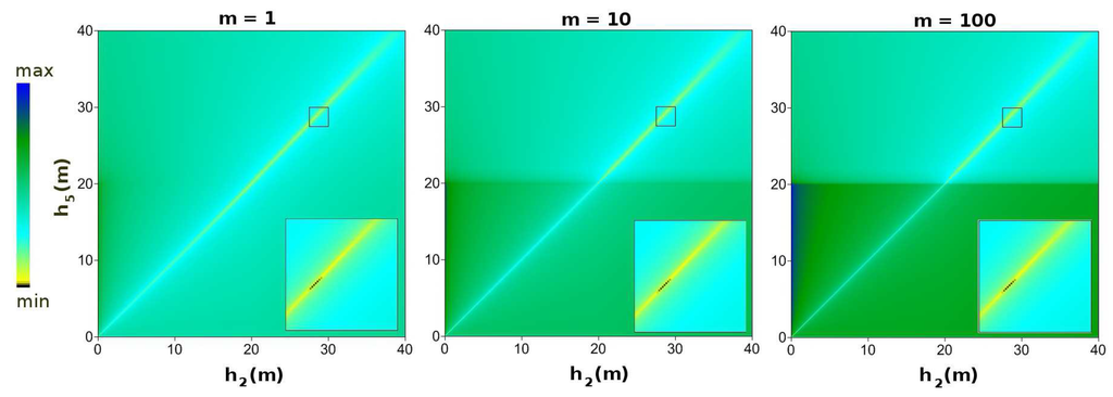
Figure 5. Map of the balance error given by Equation (17), for the approach of Doherty [3], as a function of the hydraulic heads $h_{\left(2\right)}$ (x axis) and $h_{\left(5\right)}$ (y axis), for different values of m ((left) $m=1$; (center) $m=10$; (right) $m=100$). At the bottom right corner of each graph, the zone containing the minimum error value is enlarged.

Figure 5. Map of the balance error given by Equation (17), for the approach of Doherty [3], as a function of the hydraulic heads $h_{\left(2\right)}$ (x axis) and $h_{\left(5\right)}$ (y axis), for different values of m ((left) $m=1$; (center) $m=10$; (right) $m=100$). At the bottom right corner of each graph, the zone containing the minimum error value is enlarged.

The second investigated approach was proposed by Keating and Zyvoloski [4]. Horizontal interblock transmittance is calculated as follows:

$$\begin{array}{ccc}\hfill {\mathcal{T}}_{(1,2)}& =& {\displaystyle \frac{1}{2}\left({\displaystyle \frac{{\vartheta }_{\left(1\right)}}{z_{\left(1\right)}^{\left(\mathrm{top}\right)}-z_{\left(1\right)}^{\left(\mathrm{bot}\right)}}+\frac{{\vartheta }_{\left(2\right)}}{z_{\left(2\right)}^{\left(\mathrm{top}\right)}-z_{\left(2\right)}^{\left(\mathrm{bot}\right)}}}\right)·2\frac{K_{\left(1\right)}{K}_{\left(2\right)}}{K_{\left(1\right)}+K_{\left(2\right)}}·}\hfill \\ \\ & & {\displaystyle ·\frac{1}{2}\left(z_{\left(1\right)}^{\left(\mathrm{top}\right)}-z_{\left(1\right)}^{\left(\mathrm{bot}\right)}+z_{\left(2\right)}^{\left(\mathrm{top}\right)}-z_{\left(2\right)}^{\left(\mathrm{bot}\right)}\right)\frac{\Delta y}{\Delta x}}\hfill \end{array}$$

(21)

For vertical transmittance, the change from intrinsic vertical internode conductivity in a partially-saturated cell to zero in a dry cell would lead to a discontinuity. To improve numerical stability, Keating and Zyvoloski [4] allow a weak scaling controlled by a user-specified parameter, ξ:

$$\begin{array}{ccc}\hfill {\mathcal{T}}_{(2,5)}& =& \left[min\left({\displaystyle 1,\xi \frac{{\vartheta }_{\left(2\right)}}{z_{\left(2\right)}^{\left(\mathrm{top}\right)}-z_{\left(2\right)}^{\left(\mathrm{bot}\right)}}}\right)+min\left({\displaystyle 1,\xi \frac{{\vartheta }_{\left(5\right)}}{z_{\left(5\right)}^{\left(\mathrm{top}\right)}-z_{\left(5\right)}^{\left(\mathrm{bot}\right)}}}\right)\right]·\hfill \\ \\ & & {\displaystyle ·2\frac{K_{\left(2\right)}{K}_{\left(5\right)}}{K_{\left(2\right)}+K_{\left(5\right)}}·2\frac{\Delta x\Delta y}{z_{\left(5\right)}^{\left(\mathrm{top}\right)}-z_{\left(2\right)}^{\left(\mathrm{bot}\right)}}}\hfill \end{array}$$

(22)

Keating and Zyvoloski [4] suggest using a value of 10 for ξ, which provides both accuracy and stability for all problems.

The last approach considered for this comparison exercise is implemented in the UPW Package of the MODFLOW NTW model [6], a standalone version of MODFLOW 2005 [25]. The UPW Package smooths the horizontal conductance function during wetting and drying of a cell. Using this method, horizontal interblock conductance for our test is calculated as follows, by making reference to the example of cells $\left(1\right)$ and $\left(2\right)$:

$$C_{(1,2)}^{NTW}=\left\{\begin{array}{cc}\eta \hfill & \mathrm{if}X\le 0,\hfill \\ \alpha K_{(1,2)}\left[{\displaystyle \frac{0.5A{X}^2}{\Omega }}\right]\hfill & \mathrm{if}0<X\le \Omega ,\hfill \\ \alpha K_{(1,2)}\left[AX+0.5(1-A)\right]\hfill & \mathrm{if}\Omega <X\le (1-\Omega ),\hfill \\ {\displaystyle \alpha K_{(1,2)}\left[\frac{1-0.5A{(1-X)}^2}{\Omega }\right]}\hfill & \mathrm{if}(1-\Omega )<X\le 1,\hfill \\ \alpha K_{(1,2)}\hfill & \mathrm{if}X\ge 1\hfill \end{array}\right.$$

(23)

where $X=\left(h_{\mathrm{up}}-z_{\mathrm{up}}^{\left(\mathrm{bot}\right)}\right){\left(z_{up}^{\left(top\right)}-z_{up}^{\left(\mathrm{bot}\right)}\right)}^{-1}$; $h_{\mathrm{up}}$ is the maximum between $h_{\left(1\right)}$ and $h_{\left(2\right)}$; $z_{\mathrm{up}}^{\left(\mathrm{bot}\right)}$ and $z_{\mathrm{up}}^{\left(\mathrm{top}\right)}$ are respectively the bottom and top level of the cell corresponding to $h_{\mathrm{up}}$; η is a small value, usually taken as $\eta =1\times {10}^{-9}{\text{m}}^2{\text{s}}^{-1}$; $\alpha =\left(z_{\mathrm{up}}^{\left(\mathrm{top}\right)}-z_{\mathrm{up}}^{\left(\mathrm{bot}\right)}\right)\Delta y\Delta x^{-1}$; $K_{(1,2)}$ the internode conductivity calculated as $K_{(1,2)}=2K_{\left(1\right)}{K}_{\left(2\right)}{\left(K_{\left(1\right)}+K_{\left(2\right)}\right)}^{-1}$; Ω is the smoothing interval length, which is suggested to be very small (${10}^{-5}$), and $A=\Omega {(1-\Omega )}^{-1}$.

In this approach, vertical conductance is calculated as in standard MODFLOW 2005 [25]:

$$C_{(2,5)}=2\Delta x\Delta y\frac{K_{\left(2\right)}{K}_{\left(5\right)}}{\left(h_{\left(2\right)}-z_{\left(2\right)}^{\left(\mathrm{bot}\right)}\right)K_{\left(5\right)}+\left(h_{\left(5\right)}-z_{\left(5\right)}^{\left(\mathrm{bot}\right)}\right)K_{\left(2\right)}}$$

(24)

The pumping rate is reduced as the head in the cell drops below a user-specified percentage of the cell thickness, as:

$$Q^{NWT}=\left\{\begin{array}{cc}0\hfill & \mathrm{if}\delta \le 0,\hfill \\ {\displaystyle Q\left(-2{\delta }^3+3{\delta }^2\right)}\hfill & \mathrm{if}0<\delta <1/\Phi ,\hfill \\ Q\hfill & \mathrm{if}\delta \ge 1/\Phi \hfill \end{array}\right.$$

(25)

where:

$$\delta =\frac{1}{\Phi }\frac{h-z^{\left(\mathrm{bot}\right)}}{z^{\left(\mathrm{top}\right)}-z^{\left(\mathrm{bot}\right)}}$$

and Φ is a user-specified fraction of the cell thickness, typically assigned as $\Phi =0.25$.

The results obtained with the application of the four described approaches (i.e., the three approaches described in this section and the one implemented in YAGMod), for three cases corresponding to an extraction rate Q varying from $0.1{\text{m}}^3{\text{s}}^{-1}$ to $0.2{\text{m}}^3{\text{s}}^{-1}$ and $0.3{\text{m}}^3{\text{s}}^{-1}$, are represented in Figure 6. Notice that with the approach by Keating and Zyvoloski [4], $h_{\left(5\right)}$ cannot drop below the cell bottom; therefore, the results obtained with this method for extraction rates of $0.2{\text{m}}^3{\text{s}}^{-1}$ and $0.3{\text{m}}^3{\text{s}}^{-1}$ could not be significantly compared to those from other algorithms. Besides this remark, all of the methods give realistic results, even if the values that yield the least total balance error for alternative algorithms differ from each other.

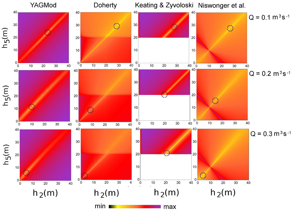
Figure 6. Map of the total quadratic balance error given by Equation (17), as a function of the hydraulic heads $h_{\left(2\right)}$ (x axis) and $h_{\left(5\right)}$ (y axis). From left to right, respectively, the results obtained with YAGMod and the approaches by Doherty [3], Keating and Zyvoloski [4] and Niswonger et al. [6]. From top down, the results obtained with extraction rates of $0.1{\text{m}}^3{\text{s}}^{-1}$, $0.2{\text{m}}^3{\text{s}}^{-1}$ and $0.3{\text{m}}^3{\text{s}}^{-1}$. The blue circles point out the zone where the least value of the total quadratic balance error is located.

Figure 6. Map of the total quadratic balance error given by Equation (17), as a function of the hydraulic heads $h_{\left(2\right)}$ (x axis) and $h_{\left(5\right)}$ (y axis). From left to right, respectively, the results obtained with YAGMod and the approaches by Doherty [3], Keating and Zyvoloski [4] and Niswonger et al. [6]. From top down, the results obtained with extraction rates of $0.1{\text{m}}^3{\text{s}}^{-1}$, $0.2{\text{m}}^3{\text{s}}^{-1}$ and $0.3{\text{m}}^3{\text{s}}^{-1}$. The blue circles point out the zone where the least value of the total quadratic balance error is located.

The hydraulic heads computed with YAGMod for an extraction rate of $0.1{\text{m}}^3{\text{s}}^{-1}$ are smaller than those obtained with the other approaches; on the other hand, for higher extraction rates, the behavior is more complex, and no systematic difference is shown.

The color scales of the plots of Figure 6 are normalized with respect to the minimum and maximum total quadratic errors, separately for each method. Therefore, the images show that all of the methods yield a single minimum, and for YAGMod, ${ϵ}_{\mathrm{tot}}^2$ increases from the least value more rapidly than for other methods.

Finally, each of the algorithms, which are here compared to YAGMod, is based on some auxiliary parameters. Such parameters are not related to physical processes or quantities, but are necessary to apply artifices to face the numerical problems arising from the simulation of drying cells. These auxiliary parameters, which are listed in Table 1, have to be assigned by the user. On the other hand, YAGMod does not require any additional parameter. This is useful to limit the arbitrariness associated with the assignment of non-physical, auxiliary quantities.

Table 1. Parameters to be assigned by the user for the algorithms with which YAGMod is compared.

Algorithm	Parameters
Doherty [3]	${\theta }_r$, f, m
Keating and Zyvoloski [4]	ξ
Niswonger et al. [6]	η, Ω, Φ

Table 1. Parameters to be assigned by the user for the algorithms with which YAGMod is compared.

Algorithm	Parameters
Doherty [3]	${\theta }_r$, f, m
Keating and Zyvoloski [4]	ξ
Niswonger et al. [6]	η, Ω, Φ

4. Inverse Modeling with the Comparison Model Method

YAGMod permits the application of the comparison model method (CMM) to estimate the conductivity field for a 2D flow field by solving an inverse problem. The CMM was proposed to identify T at every node of a discretization grid [18] and successively developed to directly compute internode transmissivities [19]. Further modifications were proposed by Ponzini and Crosta [20], Ponzini et al. [26], Pasquier and Marcotte [27], Ponzini et al. [28]. The CMM was applied to alluvial aquifers in Italy [14,16,21], Switzerland [22] and Canada [23,29,30] and to a carbonatic aquifer in southern Italy [17,31].

4.1. Fundamentals of the CMM Algorithm

In this section, we summarize the working fundamentals of the CMM for the computation of the conductivity field for 2D stationary flow. Therefore, the k index is omitted in the following equations.

The CMM requires the knowledge of a reference head field, $h_{(i,j)}^{\left(\mathrm{ref}\right)}$, which is usually obtained from the interpolation of field measurements and any other relevant geological or hydrological information. Furthermore, a reference source term has to be estimated at every cell of the domain, $F_{(i,j)}^{\left(\mathrm{ref}\right)}$, and it coincides with the same term introduced in Equation (5) (for $k=1$, as 2D flow is assumed).

Difficulties in estimating a realistic conductivity field from the application of the CMM could arise from the intrinsic instability of the inverse problem or the ill-conditioning of the discrete inverse problem [32]: these difficulties are mainly related to the behavior of the balance equation, which, when used for the forward problem, behaves as a K-to-h map, which smooths the high wavenumber (or short wavelength) components of the conductivity field. From the point of view of the inverse problem, errors on the head at high wavenumbers could be amplified, even if they have a small amplitude [33]. Therefore, it is often useful to smooth the reference head and source fields.

An initial guess of the conductivity field, $K_{(i,j)}^{\left(\mathrm{CM}\right)}$, must be assigned, for instance, by interpolating the values estimated from field tests. Then, the forward problem is solved for a comparison model (CM): the CM shares the same geometry and source terms as the model, which has to be calibrated. In particular, the forward problem aims at finding the head field, $h_{(i,j)}^{\left(\mathrm{CM}\right)}$, which solves Equation (5), for $k=1$. For the CM, $h_{(i,j)}^{\left(\mathrm{CM}\right)}=h_{(i,j)}^{\left(\mathrm{ref}\right)}$ at the nodes where Dirichlet boundary conditions are assigned.

From the results of the forward problem for the CM, the aquifer unit discharge, i.e., the water flow rate through the whole aquifer thickness per unit horizontal length, can be computed at each cell as:

$${\mathbf{Q}}_{(i,j)}^{\left(\mathrm{CM}\right)}=-K_{(i,j)}^{\left(\mathrm{CM}\right)}{\vartheta }_{(i,j)}^{\left(\mathrm{CM}\right)}\nabla h_{(i,j)}^{\left(\mathrm{CM}\right)}$$

(26)

where ${\vartheta }_{(i,j)}^{\left(\mathrm{CM}\right)}$ is computed from Equation (3), with $h_{(i,j,k)}=h_{(i,j)}^{\left(\mathrm{CM}\right)}$, and $\nabla h_{(i,j)}^{\left(\mathrm{CM}\right)}$ is the discrete gradient obtained with a classical finite difference approximation. The real aquifer unit discharge could be estimated as:

$${\mathbf{Q}}_{(i,j)}=-K_{(i,j)}{\vartheta }_{(i,j)}^{\left(\mathrm{ref}\right)}\nabla h_{(i,j)}^{\left(\mathrm{ref}\right)}$$

(27)

if the reference hydraulic head were a good approximation of the real head field, with the obvious meaning of the terms appearing in the right-hand side of this equation. If $K_{(i,j)}^{\left(\mathrm{CM}\right)}$ is a good approximation of the real K field, then it is reasonable to assume that:

$${\mathbf{Q}}_{(i,j)}^{\left(\mathrm{CM}\right)}\simeq {\mathbf{Q}}_{(i,j)}$$

(28)

If we take into account only the absolute values of the previous expression, from Equations (26) and (27), the estimated conductivity can be found as:

$$K_{(i,j)}^{\left(\mathrm{est}\right)}=K_{(i,j)}^{\left(\mathrm{CM}\right)}·\frac{{\vartheta }_{(i,j)}^{\left(\mathrm{CM}\right)}}{{\vartheta }_{(i,j)}^{\left(\mathrm{ref}\right)}}·\frac{|\nabla h_{(i,j)}^{\left(\mathrm{CM}\right)}|}{|\nabla h_{(i,j)}^{\left(\mathrm{ref}\right)}|}$$

(29)

This is called the “integral” approach of the CMM, as opposed to the “differential” approach, which considers:

$$Q_{(i,j)}=|{\mathbf{Q}}_{(i,j)}|=K_{(i,j)}{\vartheta }_{(i,j)}\left|\nabla h_{(i,j)}\right|$$

(30)

as a function of $h_{(i,j)}$, both explicitly through $|\nabla h_{(i,j)}|$ and implicitly through ${\vartheta }_{(i,j)}$. A small variation of $K_{(i,j)}$ and $h_{(i,j)}$ should produce a small variation of $Q_{(i,j)}$; this is expressed in terms of differentials as:

$$d{Q}_{(i,j)}=d{K}_{(i,j)}{\vartheta }_{(i,j)}|\nabla h_{(i,j)}|+K_{(i,j)}d{\vartheta }_{(i,j)}|\nabla h_{(i,j)}|+K_{(i,j)}{\vartheta }_{(i,j)}d\left|\nabla h_{(i,j)}\right|$$

(31)

If the couples $\left(K_{(i,j)}^{\left(\mathrm{CM}\right)},h_{(i,j)}^{\left(\mathrm{CM}\right)}\right)$ and $\left(K_{(i,j)}^{\left(\mathrm{est}\right)},h_{(i,j)}^{\left(\mathrm{ref}\right)}\right)$ are considered, respectively, as the initial and final “points”, so that $d{K}_{(i,j)}=K_{(i,j)}^{\left(\mathrm{est}\right)}-K_{(i,j)}^{\left(\mathrm{CM}\right)}$, $d{\vartheta }_{(i,j)}={\vartheta }_{(i,j)}^{\left(\mathrm{ref}\right)}-{\vartheta }_{(i,j)}^{\left(\mathrm{CM}\right)}$ and $d|\nabla h_{(i,j)}|=|\nabla h_{(i,j)}^{\left(\mathrm{ref}\right)}|-|\nabla h_{(i,j)}^{\left(\mathrm{CM}\right)}|$, and if Equation (28) holds, then $d{Q}_{(i,j)}=0$. Finally, from Equation (31), it follows:

$$K_{(i,j)}^{\left(\mathrm{est}\right)}=K_{(i,j)}^{\left(\mathrm{CM}\right)}\left(1-\frac{{\vartheta }_{(i,j)}^{\left(\mathrm{ref}\right)}-{\vartheta }_{(i,j)}^{\left(\mathrm{CM}\right)}}{{\vartheta }_{(i,j)}^{\left(\mathrm{CM}\right)}}-\frac{|\nabla h_{(i,j)}^{\left(\mathrm{ref}\right)}|-|\nabla h_{(i,j)}^{\left(\mathrm{CM}\right)}|}{|\nabla h_{(i,j)}^{\left(\mathrm{CM}\right)}|}\right)$$

(32)

which is the expression of the estimated conductivity with the “differential” approach of the CMM.

The CMM can be modified and recast in an iterative fashion, to progressively improve the fit of the reference data. This is done by using $\ell =0,1,\dots$ as the iteration index, by assuming a given initial guess $K_{(i,j)}^{\left(0\right)}$, and by substituting $K_{(i,j)}^{\left(\mathrm{est}\right)}$ with $K_{(i,j)}^{(\ell +1)}$, $K_{(i,j)}^{\left(\mathrm{CM}\right)}$ with $K_{(i,j)}^{\left(\ell \right)}$ and $h_{(i,j)}^{\left(\mathrm{CM}\right)}$ with $h_{(i,j)}^{\left(\ell \right)}$ in Equations (29) and (32).

It is often useful to weight the correction introduced at each iteration with $w=min\left(c\right|\nabla h_{(i,j)}^{\left(\mathrm{ref}\right)}|,1)$, where c is a positive constant, in order to avoid the excessive growth of some values where the reference hydraulic gradient is small and, therefore, the problem ill-conditioned:

$$K_{(i,j)}^{(\ell +1)}=K_{(i,j)}^{\left(\ell \right)}\left[w·\left(\frac{{\vartheta }_{(i,j)}^{\left(\ell \right)}}{{\vartheta }_{(i,j)}^{\left(\mathrm{ref}\right)}}·\frac{|\nabla h_{(i,j)}^{\left(\ell \right)}|}{|\nabla h_{(i,j)}^{\left(\mathrm{ref}\right)}|}-1\right)+1\right]$$

(33)

for the integral approach and:

$$K_{(i,j)}^{(\ell +1)}=K_{(i,j)}^{\left(\ell \right)}\left[1-w·\left(\frac{{\vartheta }_{(i,j)}^{\left(\mathrm{ref}\right)}-{\vartheta }_{(i,j)}^{\left(\ell \right)}}{{\vartheta }_{(i,j)}^{\left(\ell \right)}}+\frac{|\nabla h_{(i,j)}^{\left(\mathrm{ref}\right)}|-|\nabla h_{(i,j)}^{\left(\ell \right)}|}{|\nabla h_{(i,j)}^{\left(\ell \right)}|}\right)\right]$$

(34)

for the differential approach.

4.2. A Test

A simple test is used to show the application of the CMM. In particular, the reference K field is represented in Figure 7 (left image) for a domain with $10\times 10$ cells and corresponds to a conductive inclusion in a less permeable domain. The reference hydraulic head is obtained by solution of the forward problem with Dirichlet boundary conditions and is represented by the image map in Figure 8. The results obtained from the CMM with a homogeneous initialization $K^{\left(\mathrm{CM}\right)}={10}^{-4}\text{m}{\text{s}}^{-1}$ are shown in Figure 7, both for the integral (central map) and the differential (right map) approaches.

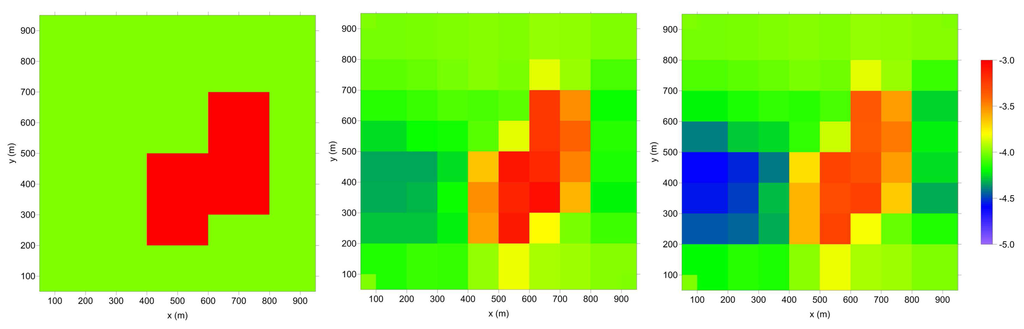
Figure 7. Simple test of the comparison model method (CMM): hydraulic conductivity field; the color scale refers to ${log}_{10}K$, with K expressed in $\text{m}{\text{s}}^{-1}$. (left) Reference field; (central) field estimated from the CMM with the integral approach; (right) field estimated from the CMM with the differential approach.

Figure 7. Simple test of the comparison model method (CMM): hydraulic conductivity field; the color scale refers to ${log}_{10}K$, with K expressed in $\text{m}{\text{s}}^{-1}$. (left) Reference field; (central) field estimated from the CMM with the integral approach; (right) field estimated from the CMM with the differential approach.

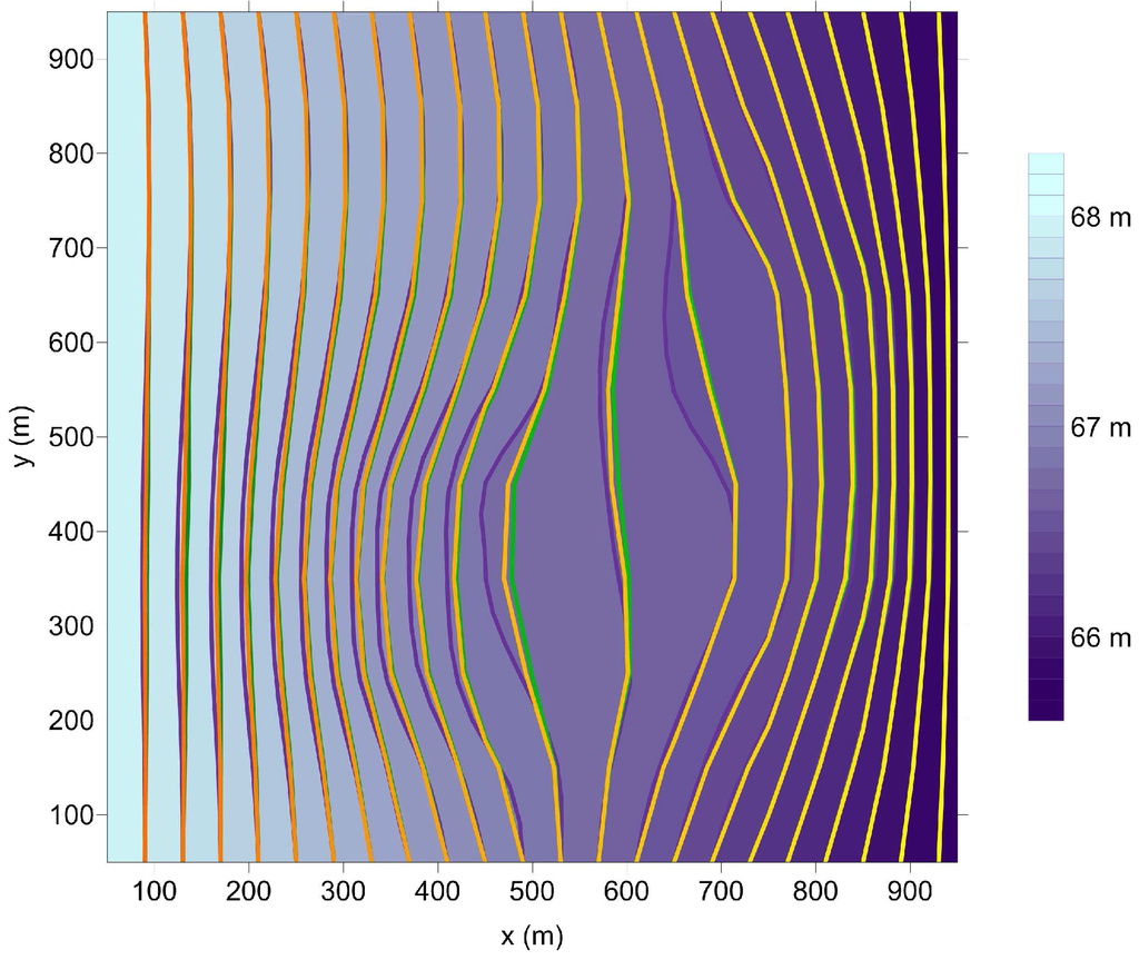
Figure 8. Simple test of the CMM: image plot of the reference hydraulic head and contour lines of the reference h field (purple) and of the h fields obtained for the K fields estimated with the CMM: yellow lines refer to the K field obtained with the integral approach (central map of Figure 7) and green lines to the K field obtained with the differential approach (right map of Figure 7).

Figure 8. Simple test of the CMM: image plot of the reference hydraulic head and contour lines of the reference h field (purple) and of the h fields obtained for the K fields estimated with the CMM: yellow lines refer to the K field obtained with the integral approach (central map of Figure 7) and green lines to the K field obtained with the differential approach (right map of Figure 7).

The high conductivity region is quite well reproduced by the CMM, although it is a little bit faint, an effect that depends on the spectral response of the balance equation: this induces also some small differences between the water head computed from the K fields estimated with the CMM and the reference h field (see Figure 8), above all around the border of the high conductivity region.

5. Conclusions

Yet another groundwater flow model, YAGMod, has been described in this paper. The basic characteristics of this model are briefly summarized below.

• When the water head in a cell is lower than the cell’s top coordinate, the cell is considered as partially saturated, and its saturated thickness is used for the water balance. If the water head is lower than the cell bottom, then the cell is considered as dry, but it is not excluded from the water balance calculations. In fact, the water head in this cell is used to compute a vertical water balance that permits one to transfer source terms (namely, aquifer recharge) from the shallow layers down to the deep ones.
• A large number of different sources or boundary conditions, which depend on the water head in the cell, are simulated with a single prototype equation.
• If the position of the screened intervals of a water abstraction well is known, the extraction rate can be limited when the water head falls within the screened interval or turned off when the water head falls below the bottom of the screens.

The comparison of the algorithm used by YAGMod and those proposed by Doherty [3], Keating and Zyvoloski [4] and Niswonger et al. [6] shows that the different approaches yield different solutions, among which, it is not possible to select the best one on the basis of physical arguments. Nevertheless, the advantage of YAGMod is that it does not introduce any additional parameter whose values should be assigned by the user and which mostly have a limited physical significance. Differently, the other approaches require that the user defines one or more additional parameters. These parameters mostly have a limited physical significance, making the parameterization of the model more complex.

Moreover, YAGMod can be used also to solve the inverse problem with the CMM for a phreatic aquifer, with either an integral or a differential approach and taking into account the variability of saturation. This further strengthens the features of YAGMod, because the CMM is embedded in the source code and can be applied to estimate the hydraulic conductivity field, directly at the model scale. The present version of YAGMod is developed to apply the CMM with 2D flow fields, but it can be easily extended to 3D flows, if data with high quality and high density are available.

YAGMod is sufficiently flexible to be adapted to other situations, as was done to model groundwater flow in multi-layered coastal aquifers by De Filippis et al. [31], who modified YAGMod to cope with the variable thickness of the aquifer saturated with fresh water and to identify the spatial variability of a fractured and karst carbonatic aquifer with the application of the CMM to a single layer, while the parameters of other layers are fixed with estimates based on prior information.

The strategy used by YAGMod to cope with draining cells can be easily applied to integrated finite differences [34], but can be adapted also to other numerical techniques, which are based on the discretization of the integral balance equation over a given subdomain.

References

- Bear, J. Hydraulics of Groundwater; Springer-Verlag: New York, NY, USA, 1979; p. 567. [Google Scholar]
- De Marsily, G. Quantitative Hydrogeology—Groundwater Hydrology for Engineers; Academic Press: New York, NY, USA, 1986. [Google Scholar]
- Doherty, J. Improved calculations for dewatered cells in MODFLOW. Groundwater 2001, 39, 863–869. [Google Scholar]
- Keating, E.; Zyvoloski, G. A stable and efficient numerical algorithm for unconfined aquifer analysis. Groundwater 2009, 47, 569–579. [Google Scholar]
- Bedekar, V.; Niswonger, R.G.; Kipp, K.; Panday, S.; Tonkin, M. Approaches to the simulation of unconfined flow and perched groundwater flow in MODFLOW. Groundwater 2012, 50, 187–198. [Google Scholar]
- Niswonger, R.G.; Panday, S.; Ibaraki, M. MODFLOW-NWT, a Newton Formulation for MODFLOW-2005; US Geological Survey Techniques and Methods; USGS: Reston, VA, USA, 2011; Volume 6, p. A37.
- Ponzini, G.; Crosta, G.; Giudici, M. The hydrogeological role of an aquitard in preventing drinkable water well contamination: A case study. Environ. Health Perspect. 1989, 83, 77–95. [Google Scholar]
- Bersezio, R.; Bini, A.; Giudici, M. Effects of sedimentary heterogeneity on groundwater flow in a quaternary pro-glacial delta environment: Joining facies analysis and numerical modelling. Sediment. Geol. 1999, 129, 327–344. [Google Scholar]
- Giudici, M.; Foglia, L.; Parravicini, G.; Ponzini, G.; Sincich, B. A quasi three dimensional model of water flow in the subsurface of Milano (Italy): The stationary flow. Hydrol. Earth Syst. Sci. 2000, 4, 113–124. [Google Scholar]
- Valota, G.; Giudici, M.; Parravicini, G.; Ponzini, G.; Romano, E. Is the forward problem of ground water hydrology always well posed? Ground Water 2002, 40, 500–508. [Google Scholar]
- Zappa, G.; Bersezio, R.; Felletti, F.; Giudici, M. Modeling heterogeneity of gravel-sand, braided stream, alluvial aquifers at the facies scale. J. Hydrol. 2006, 325, 134–153. [Google Scholar]
- Felletti, F.; Bersezio, R.; Giudici, M. Geostatistical simulation and numerical upscaling, to model ground water flow in a sandy-gravel, braided river, aquifer analogue. J. Sediment. Res. 2006, 76, 1215–1229. [Google Scholar]
- Giudici, M.; Ponzini, G.; Romano, E.; Vassena, C. Some lessons from modelling ground water flow in the metropolitan area of Milano (Italy) at different scales. Mem. Descr. Della Carta Geol. d’Italia 2007, 76, 207–218. [Google Scholar]
- Vassena, C.; Durante, C.; Giudici, M.; Ponzini, G. The importance of observations on fluxes to constrain ground water model calibration. Phys. Chem. Earth A B C 2008, 33, 1105–1110. [Google Scholar]
- Vassena, C.; Cattaneo, L.; Giudici, M. Assessment of the role of facies heterogeneity at the fine scale by numerical transport experiments and connectivity indicators. Hydrogeol. J. 2010, 18, 651–668. [Google Scholar]
- Vassena, C.; Rienzner, M.; Ponzini, G.; Giudici, M.; Gandolfi, C.; Durante, C.; Agostani, D. Modeling water resources of an highly irrigated alluvial plain: Coupling and calibrating soil and ground water models. Hydrogeol. J. 2011, 20, 449–467. [Google Scholar]
- Giudici, M.; Margiotta, S.; Mazzone, F.; Negri, S.; Vassena, C. Modeling hydrostratigraphy and groundwater flow of a fractured and karst aquifer in a Mediterranean basin (Salento peninsula, southeastern Italy). Environ. Earth Sci. 2012, 67, 1891–1907. [Google Scholar]
- Scarascia, S.; Ponzini, G. An approximate solution for the inverse problem in hydraulics. L’Energia Elettr. 1972, 49, 518–531. [Google Scholar]
- Ponzini, G.; Lozej, A. Identification of aquifer transmissivities: The comparison model method. Water Resour. Res. 1982, 18, 597–622. [Google Scholar] [CrossRef]
- Ponzini, G.; Crosta, G. The comparison model method: A new arithmetic approach to the discrete inverse problem of groundwater hydrology, 1, One-dimensional flow. Transp. Porous Media 1988, 3, 415–436. [Google Scholar] [CrossRef]
- Associazione Irrigazione Est Sesia. Le Acque Sotterranee Della Pianura Irrigua Novarese-Lomellina. Studi e Ricerche Per La Realizzazione di un Modello Gestionale (Subsurface Water of Irrigated Novara-Lomellina Plain. Study and Research for a Managing Model Realization.); Report; Associazione Irrigazione Est Sesia: Novara, Italy, 1979. (In Italian) [Google Scholar]
- Beatrizotti, G.; Hansen, W.J.; Spocci, R. Optimierung der Benötigten daten für ein numerisches Modell der Grundwasserbewirtschaftung im Lockergestein (Optimization of the required data for a numerical model of groundwater management in soil). Gas Wasser Abwasser 1983, 63, 469–476. (In German) [Google Scholar]
- Benoit, N.; Pasquier, P.; Marcotte, D.; Nastev, M. Conditional stochastic inverse modelling of the Châteauguay river aquifers. In Proceedings of the ModelCARE 2005, The Hague (Scheveningen), The Netherlands, 6–9 June 2005; pp. 515–521.
- Hill, M.C.; Kavetski, D.; Clark, M.; Ye, M.; Arabi, M.; Lu, D.; Foglia, L.; Mehl, S. Practical Use of Computationally Frugal Model Analysis Methods. Groundwater 2015. [Google Scholar] [CrossRef] [PubMed]
- Harbaugh, A.W. MODFLOW-2005, the US Geological Survey Modular Ground-Water Model: The Ground-Water Flow Process; US Department of the Interior, US Geological Survey: Reston, VA, USA, 2005.
- Ponzini, G.; Crosta, G.; Giudici, M. Identification of thermal conductivities by temperature gradient profiles: One-dimensional steady state flow. Geophysics 1989, 54, 643–653. [Google Scholar] [CrossRef]
- Pasquier, P.; Marcotte, D. Steady- and transient-state inversion in hydrogeology by successive flux estimation. Adv. Water Resour. 2006, 29, 1934–1952. [Google Scholar] [CrossRef]
- Ponzini, G.; Giudici, M.; Vassena, C. Comment to “Steady- and transient-state inversion in hydrogeology by successive flux estimation” by P. Pasquier and D. Marcotte. Adv. Water Resour. 2007, 30, 2051–2053. [Google Scholar] [CrossRef]
- Pasquier, P. Résolution du probléme inverse en hydrogéologie par une estimation successive des flux (Solving hydrogeological inverse problem by successive flux estimation). Ph.D. Thesis, École Polytechnique de Montréal, Montréal, QC, Canada, 2005. [Google Scholar]
- Pasquier, P.; Marcotte, D. Solving the Groundwater Inverse Problem by Successive Flux Estimation. In Proceedings of the Fifth European Conference on Geostatistics for Environmental Applications; Renard, P., Demougeot-Renard, H.F.R., Eds.; Springer Verlag: Berlin, Germany, 2005. [Google Scholar]
- De Filippis, G.; Giudici, M.; Negri, S.; Margiotta, S. Conceptualization and preliminary characterization of a karst, coastal aquifer in the Mediterranean area of the Taranto gulf (southern Italy). Environ. Earth Sci. 2015. submitted. [Google Scholar]
- Giudici, M.; Ginn, T.; Vassena, C.; Haeri, H.; Foglia, L. A critical review of the properties of forward and inverse problems in groundwater hydrology. In Calibration and Reliability in Groundwater Modelling: Credibility of Modelling; Refsgaard, J., Kovar, K., Haarder, E., Nygaard, E., Eds.; IAHS: Wallingford, UK, 2008; Volume 320, pp. 240–244. [Google Scholar]
- Giudici, M.; Vassena, C. Spectral analysis of the balance equation of ground water hydrology. Transp. Porous Media 2008, 72, 171–178. [Google Scholar] [CrossRef]
- Narasimhan, T.N.; Witherspoon, P.A. An integrated finite difference method for analyzing fluid flow in porous media. Water Resour. Res. 1976, 12, 57–64. [Google Scholar] [CrossRef]
© 2015 by the authors; licensee MDPI, Basel, Switzerland. This article is an open access article distributed under the terms and conditions of the Creative Commons by Attribution (CC-BY) license (http://creativecommons.org/licenses/by/4.0/).