Bonding Strength Effects in Hydro-Mechanical Coupling Transport in Granular Porous Media by Pore-Scale Modeling

Abstract

The hydro-mechanical coupling transport process of sand production is numerically investigated with special attention paid to the bonding effect between sand grains. By coupling the lattice Boltzmann method (LBM) and the discrete element method (DEM), we are able to capture particles movements and fluid flows simultaneously. In order to account for the bonding effects on sand production, a contact bond model is introduced into the LBM-DEM framework. Our simulations first examine the experimental observation of “initial sand production is evoked by localized failure” and then show that the bonding or cement plays an important role in sand production. Lower bonding strength will lead to more sand production than higher bonding strength. It is also found that the influence of flow rate on sand production depends on the bonding strength in cemented granular media, and for low bonding strength sample, the higher the flow rate is, the more severe the erosion found in localized failure zone becomes.

1. Introduction

Sand production is commonly observed during the extrusion of hydrocarbons from reservoirs, which makes a great of trouble in oil or gas production [1]. It was reported that 70% of the world’s gas or oil reservoir has the potential risk to produce sand during their production life [1,2]. As a result, the petroleum industry spends millions of dollars each year to find ways to solve this problem [3].

In the past few decades, some achievements on sand production have been made by experimental studies, among which two mechanisms about sand production are convincing [4,5]. Firstly, the initial sand production is evoked by localized failure near the cavity owing to concentration of external stress, which is called as mechanical instability. Secondly, this localized failure zone is eroded by flow, which is named hydro-mechanical instability. Furthermore, these two mechanisms are often coupled with each other, which leads to the complexity of sand production. However, owing to the limitation in observing and measuring the micro-information about fluid and sand grains interaction by experiment, the micro underlying physics of these mechanisms is still not clear.

Therefore, numerical studies are of great importance. For a reliable numerical model for sand production, three aspects should be considered: an efficient method to capture the elastic and plastic behavior of granular media, a good description of fluid flow, and an accurate way to consider the fluid–solid interaction. In the previous numerical studies of sand production, continuum model and discrete element method are two popular approaches [3]. For continuum method, granular media is regarded as a deformable pore-elastic or pore-elastoplastic solid described by the constitutive equation [6]. However, continuum models have difficulty completely capturing the performance of granular media due to its inherent discrete nature. Meanwhile, little micro information can be obtained in continuum method to explore the mechanism at particle scale [7]. As an alternative method, the discrete element method (DEM) [8] is an efficient way to overcome those shortcomings. Firstly, DEM can capture the discrete nature of rock by treating it as an assembly of discrete particles. Secondly, DEM is based on the particle scale and the influence of micro parameters on the macroscopic behaviors can be considered, which is important for studying mechanism of sand production. Owing to these advantages, DEM was widely used to study sand production [9,10,11,12,13].

In DEM simulation of sand production, the description of fluid dynamics plays an important role. In earlier works, flow in granular media was described by Darcy’s law, which was coupled with DEM by some empirical formulas [9,10,13]. However, in Darcy-DEM models, flow in granular media cannot be calculated accurately, so CFD-DEM model was developed, where Navier–Stokes equations based on the local mean values over a computation cell were solved [11,12]. Zhou et al. [11] employed this approach to simulate the liquid-induced erosion in a weakly bonded granular media and captured the main features of the sand erosion. Compared with Darcy-DEM model, some progress has been made in CFD-DEM model, but empirical equations are again usually introduced to calculate hydrodynamic force on solid. In addition, due to the fact that hydrodynamic force acting on sand plays a critical role in sand production, the fluid–particle interaction must be evaluated at the particle scale or smaller [14], which means that CFD-DEM model is also not accurate enough to explore the underlying physics of sand production, especially about the fluid and sand grains interaction.

In the past three decades, the lattice Boltzmann method (LBM) has gained much popularity due to its efficiency in dealing with complex-boundary problems [15,16,17,18]. It has also been coupled with DEM to simulate particle-fluid system at pore scale [19,20,21]. In LBM-DEM model, the flow is calculated at pore scale, so that assumptions about the dependence between porosity and permeability are no longer needed. Therefore, the LBM-DEM model is outstanding among other numerical methods, and has been applied to study sand production process [7,14,22,23].

Boutt et al. [7] and Ghassemi et al. [22] simulated sand production in two dimensions (2D) with a coupled LBM-DEM model, and discussed the influence of the confining pressure and flow rate on sand production. In their models, the granular media is un-cemented, so there is no bonding effect between particles, and the only resistance for particle motion is friction. However, in cemented reservoir, the bonding effect is a primary property determining the macroscopic behavior of granular media, such as sandstone, and the failure of cemented granular media is generally owing to the bond breakage [24]. It was also reported that behavior of un-cemented granular media is evidently distinct from cemented granular media owing to the bonding effects between grains [25], so the conclusion obtained from un-cemented granular media may be not suitable for cemented granular media. Moreover, only limited literatures were found to simulate sand production of cemented granular media at pore scale, although some sand production experiments have been carried out for a better understanding of sand production process in cemented reservoir [2,26]. To bridge this gap, we study sand production in cemented reservoir, with special focus on the influence of bonding effect. In this paper, the LBM and DEM in a two-dimensional domain are coupled to simulate fluid–solid system, and in order to consider the effect of bonding strength, a contact bond model is incorporated in LBM-DEM framework.

The rest of this paper is organized as follows. Firstly, the numerical methods are introduced in Section 2, which includes the lattice Boltzmann method, discrete element method with contact bond model, and coupling of these two methods. In Section 3, the LBM-DEM code is validated by simulating the sedimentation of circular particles in a channel. Section 4 is the numerical results and discussion, which contains two parts: biaxial compression simulation and sand production simulation where the influence of bonding strength on sand production is discussed. Section 5 concludes the paper.

2. Numerical Methods

This section is a brief introduction of numerical methods used in our simulation: the lattice Boltzmann method for fluid phase and the discrete element method with contact bond model. The approach to couple these two methods is described at the end of this section.

2.1. Lattice Boltzmann Method (LBM)

LBM is an efficient numerical scheme to simulate fluid especially with complicated boundary condition [16,17,27,28,29,30,31,32] and multiphase interfaces [15,33,34,35,36,37]. Recently, LBM has been used to simulate fluid-solid coupling system [19,20,38,39,40,41] owing to its high efficiency compared with traditional methods.

The basic variable in LBM is density distribution function f_i. A widespread LBM implementation in the literature is the lattice Bhatnagar–Gross–Krook (LBGK) model, where the collision operator is simplified as a linearized version by assuming that the collision operator relaxes the local particle distribution functions at a single rate [15]. The evolution equation of “LBGK” model can be written as [15]:

$$f_i\left(\mathit{x}+{\mathit{e}}_{\mathit{i}}{\mathsf{\delta }}_t,t+{\delta }_t\right)=f_i\left(\mathit{x},t\right)-\frac{1}{\mathsf{\tau }}\left(f_i\left(\mathit{x},t\right)-f_i^{eq}\left(\mathit{x},t\right)\right)$$

(1)

where f_i is the distribution function in the ith discrete velocity direction ${\mathit{e}}_{\mathit{i}}$, $f_i^{eq}$ is the corresponding equilibrium distribution function, ${\mathsf{\delta }}_t$ is the time step, and τ is the relaxation time related to the fluid kinematic viscosity:

$$\mathsf{\upsilon }=\left(\mathsf{\tau }-0.5\right)c^2{\mathsf{\delta }}_t/3$$

(2)

where $c={\mathsf{\delta }}_x/{\mathsf{\delta }}_t$ is the lattice speed with ${\mathsf{\delta }}_x$ representing the lattice size, i.e., the space step. For a two-dimensional nine-speed (D2Q9) model, they are

$$\{\begin{array}{l}{e}_o=\left(0,0\right),\\ e_1=c\left(1,0\right),& e_2=c\left(1,1\right),& e_3=c\left(0,1\right),& e_4=c\left(-1,1\right),\\ e_5=c\left(-1,0\right)& e_6=c\left(-1,-1\right),& e_7=c\left(0,-1\right),& e_8=c\left(1,-1\right).\end{array}$$

(3)

The equilibrium distribution for two-dimensional nine-speed (D2Q9) model can be given as:

$$f_i^{eq}\left(\mathsf{\rho },\mathit{u}\right)=\mathsf{\rho }{\mathsf{\omega }}_i\left[1+\frac{3{\mathit{e}}_{\mathit{i}}\cdot \mathit{u}}{c^2}+\frac{9{\left({\mathit{e}}_{\mathit{i}}\cdot \mathit{u}\right)}^2}{2c^4}-\frac{3\mathit{u}\cdot \mathit{u}}{2c^2}\right]$$

(4)

where the weighting factors are:

$${\mathsf{\omega }}_i\{\begin{array}{cc}\frac{4}{9},& i=0,\\ \frac{1}{9},& i=1,3,5,7,\\ \frac{1}{36},& i=2,4,6,8.\end{array}$$

(5)

The fluid density and momentum can be obtained from the discrete distribution function,

$$\mathsf{\rho }={\displaystyle \sum _i{f}_i}$$

(6)

$$\mathsf{\rho }\mathit{u}={\displaystyle \sum _i{f}_i}{\mathit{e}}_{\mathit{i}}$$

(7)

and the pressure (p) is given by:

$$p=c^2\mathsf{\rho }/3$$

(8)

2.2. Discrete Element Method (DEM)

Discrete element method (DEM) was proposed in 1979 [8] and has been widely used in geomechanics. In our model, the classic linear spring-dashpot contact model is used [8]. The force-displacement relationship is given by:

$$F_n=-k_n\mathsf{\alpha }-C_n{\mathsf{\nu }}_n$$

(9)

$$F_s=-k_s\mathsf{\eta }-C_s{\mathsf{\nu }}_s$$

(10)

where $F_n$ is the normal contact force, $F_s$ the tangential contact force, $k_n$ the normal spring stiffness, $k_s$ the tangential spring force, $C_n$ the normal damping, and $C_s$ the tangential damping. The shear slider will work at the contact point, when $F_n$ and $F_s$ satisfy the following inequality:

$$F_s\ge \mathsf{\mu }{F}_n$$

(11)

where μ is the coefficient of friction.

The motion of the particle is described by:

$$m\frac{d^2\mathit{X}}{d{t}^2}=\mathit{F}$$

(12)

$$I\frac{d^2\mathit{\phi }}{d{t}^2}=\mathit{M}$$

(13)

where $m$ is particle mass, $\mathit{F}$ the total force acting on it, $I$ the rotation inertia, and $\mathit{M}$ is the total torque. In this work the explicit Verlet algorithm is applied, which is often used in DEM and MD simulation [42]. LBM-DEM coupling at each time step is realized by computing the fluid field by LBM firstly and then the hydrodynamic force and contact force between solids are calculated. Finally, different external forces are added together to update the particle position by integrating the above differential equation. The computation of LBM-DEM coupling is shown in Figure 1.

In order to consider the bonding effect in cemented granular media, the contact bond model is incorporated into the DEM, which is simple but can efficiently capture bonding effect between particles [43]. In this model, the bond behavior is decided by the normal bonding strength $R_n$ and the tangential bonding strength $R_t$, and $R_t$ is set equal to $R_n$. For two contacting particles, the failure envelope can be summarized by:

$$N_s=R_n$$

(14)

$$T_s=\{\begin{array}{l}{R}_t\mathrm{if}-R_n<F_n\le R_t/\mathsf{\mu },\hfill \\ \mathsf{\mu }{F}_n\mathrm{if}{F}_n>R_t/\mathsf{\mu },\hfill \end{array}$$

(15)

where $N_s$ is the normal strength, and $T_s$ is the tangential strength. The detail about this model can be found in [43].

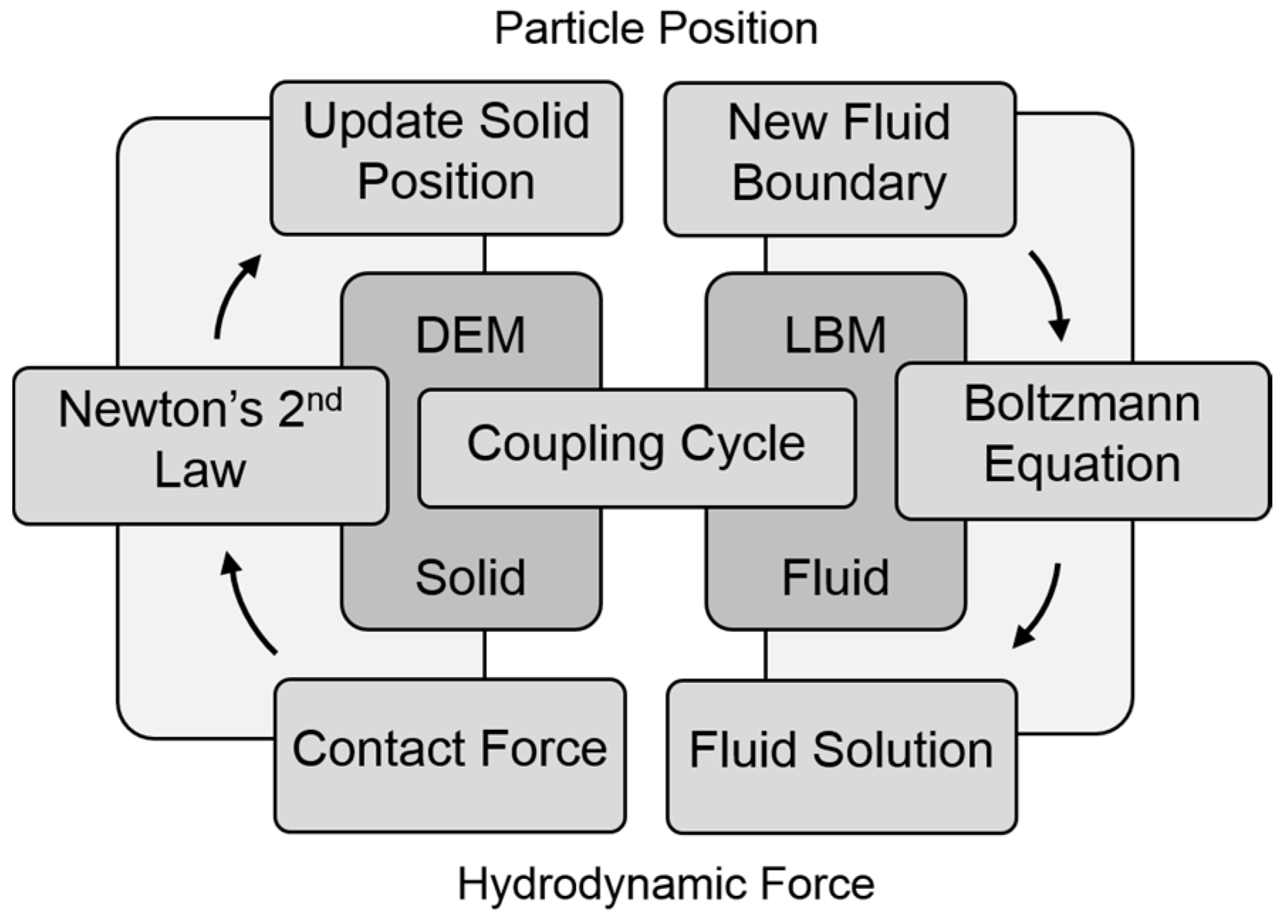
2.3. Fluid and Solid Interaction

Midway bounce-back boundary condition is applied in this work, which is easy to be implemented and widely used in particle suspension model [19]. For a moving wall, an additional term is added into the classic bounce-back procedure to keep nonslip boundary condition:

$$f_{\overline{\mathsf{\alpha }}}\left({\mathit{x}}_{\mathit{f}},t+\mathsf{\delta }t\right)={\tilde{f}}_{\mathsf{\alpha }}({\mathit{x}}_{\mathit{f}},t)-2{\mathsf{\omega }}_{\mathsf{\alpha }}\mathsf{\rho }\frac{{\mathit{e}}_{\mathit{\alpha }}\cdot {\mathit{u}}_{\mathit{w}}}{c_s^2}$$

(16)

where ${\mathit{u}}_{\mathit{w}}$ is the velocity on the midpoint of the boundary link, ${\mathit{x}}_{\mathit{f}}$ is the fluid node next to the solid, ${\mathit{e}}_{\mathit{\alpha }}$ the direction from fluid node to solid node, ${\mathit{e}}_{\overline{\mathit{\alpha }}}$ its opposite direction, and $\tilde{f}$ is the post-collision distribution function.

The calculation of hydrodynamic force is a major topic in particle suspension simulation. Ladd proposed a shell model basing on momentum exchange, where the hydrodynamic force between fluid and solid is calculated on each boundary link [19]:

$$\mathsf{\delta }{\mathit{F}}_{\mathit{w}}\left({\mathit{x}}_{\mathit{w}},{\mathit{e}}_{\mathit{\alpha }}\right)=-\left[f_{\overline{\mathsf{\alpha }}}\left({\mathit{x}}_{\mathit{f}},t\right){\mathit{e}}_{\overline{\mathit{\alpha }}}-{\tilde{f}}_{\mathsf{\alpha }}({\mathit{x}}_{\mathit{f}},t){\mathit{e}}_{\mathit{\alpha }}\right]$$

(17)

The total hydrodynamic force acting on the particle is the sum of $\mathsf{\delta }{\mathit{F}}_{\mathit{w}}\left({\mathit{x}}_{\mathit{w}},{\mathit{e}}_{\mathit{\alpha }}\right)$ on each boundary link of the particle surface:

$${\mathit{F}}_{\mathit{w}}={\displaystyle \sum \mathsf{\delta }{\mathit{F}}_{\mathit{w}}\left({\mathit{x}}_{\mathit{w}},{\mathit{e}}_{\mathit{\alpha }}\right)}$$

(18)

The corresponding total torque can be given by:

$${\mathit{T}}_{\mathit{w}}={\displaystyle \sum \left({\mathit{x}}_{\mathit{w}}-\mathit{R}\right)\times \mathsf{\delta }{\mathit{F}}_{\mathit{w}}\left({\mathit{x}}_{\mathit{w}},{\mathit{e}}_{\mathit{\alpha }}\right)}$$

(19)

where R is the mass center of the particle.

In Ladd’s model [19], the fluid exists inside and outside of the particle boundary, so it is actually a shell model and the momentum exchange is calculated for both interior and exterior fluid. As a result, the interior fluid may have an influence on the particle motion [38]. Thus, Aidun et al. [20] proposed a non-shell model by excluding the interior fluid, and the momentum exchange is only considered for exterior fluid. As Aidun suggested, for non-shell model a named “impulse force” should be added to the conventional momentum exchange method. This “impulse force” is only calculated when the particle moves to cover or uncover a lattice node, which serves as a correction for the hydrodynamic force and the necessity of this correction for non-shell model has been confirmed by [44]. Thus in our simulation the non-shell model is applied and the “impulse force” is used as a correction. When the particle moves across a fluid node the “impulse force” is written as [20]:

$${\displaystyle \sum _{CN}{\mathit{F}}_c\left(x_{\mathrm{cov}er}\right)}={\displaystyle \sum _{CN}\mathsf{\rho }\mathit{U}}$$

(20)

$${\displaystyle \sum _{CN}{\mathit{T}}_c\left(x_{\mathrm{cov}er}\right)}={\displaystyle \sum _{CN}\left({\mathit{x}}_{\mathit{c}\mathit{o}\mathit{v}\mathit{e}\mathit{r}}-\mathit{R}\right)\times {\mathit{F}}_{\mathit{c}}\left(x_{\mathrm{cov}er}\right)}$$

(21)

$${\displaystyle \sum _{UN}{\mathit{F}}_{\mathit{u}}\left(x_{uncover}\right)}=-{\displaystyle \sum _{UN}\mathsf{\rho }\mathit{U}}$$

(22)

$${\displaystyle \sum _{UN}{\mathit{T}}_{\mathit{u}}\left(x_{un\mathrm{cov}er}\right)}={\displaystyle \sum _{UN}\left({\mathit{x}}_{\mathit{u}\mathit{n}\mathit{c}\mathit{o}\mathit{v}\mathit{e}\mathit{r}}-\mathit{R}\right)\times {\mathit{F}}_{\mathit{u}}\left(x_{un\mathrm{cov}er}\right)}$$

(23)

where CN and UN are respectively fluid nodes being covered and uncovered during a time step.

3. Benchmarks

To validate the algorithm and the code, two benchmark cases are considered: single particle sedimentation, and two-particle sedimentation. For single particle sedimentation, we replicate the results computed by Feng et al. [45] using the finite element method (FEM), which is often used to validate the fluid–solid coupling methods [20,46,47]. For two-particle sedimentation, our results capture the important phenomena named “drafting, kissing and tumbling” or DKT motion [46,47], and agree well with their results quantitatively. For the consideration of stability and accuracy, the dimensionless relaxation time (τ) in LBM is taken as 1, and a relatively high grid resolution (each particle consisting of 64 LBM grids) is applied to reduce the influence of no smoothness brought by midway bounce-back model. In a 2D system, a high grid resolution can be afforded, while it may be computationally expensive for 3D. As an alternative, some smoothing models can be used such as the immersed moving boundary method [41].

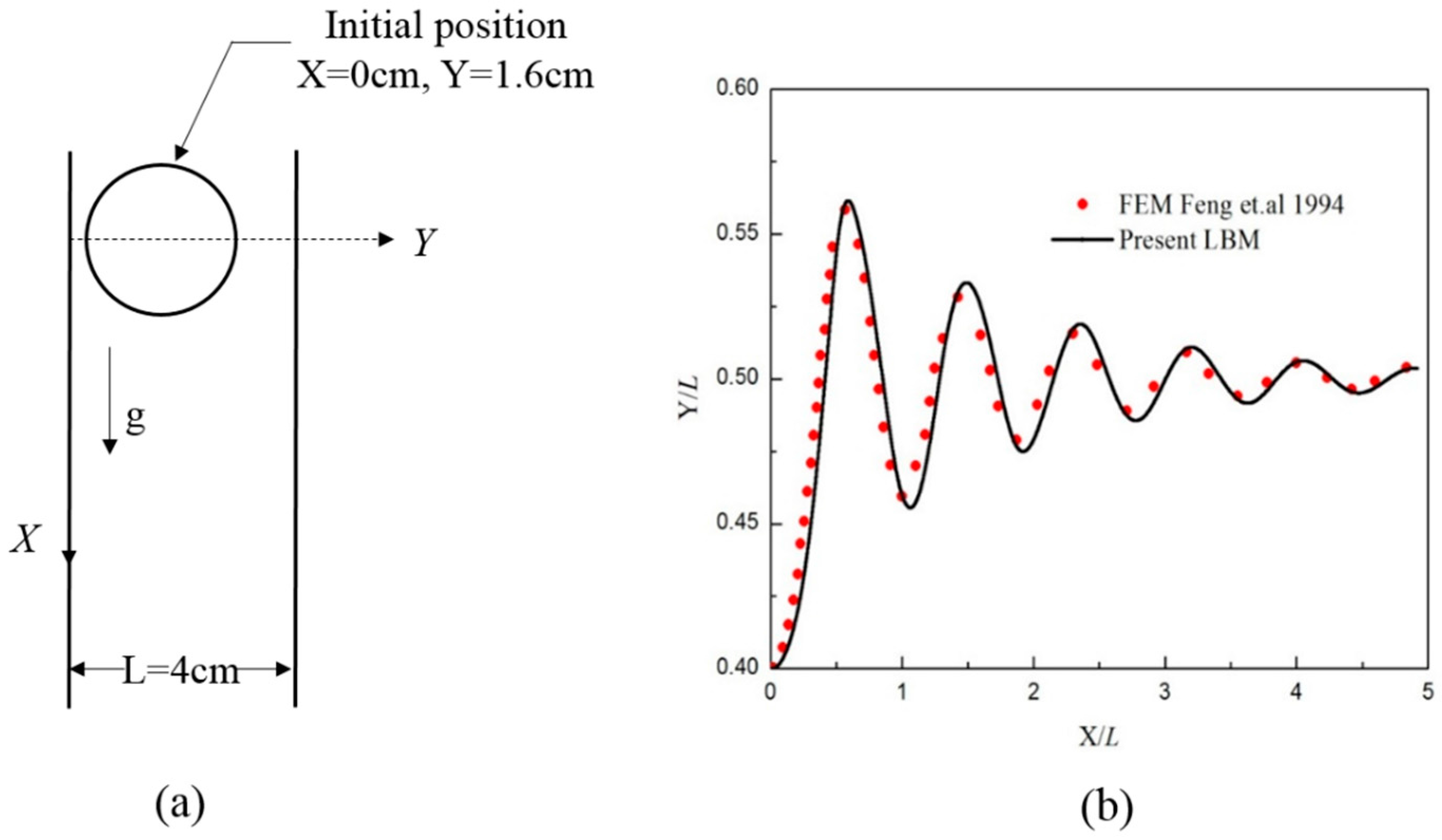
3.1. Single Particle Sedimentation

Single particle sedimentation geometry is shown in Figure 2a, where $d$ is the particle diameter, and $l=1.5d=4\mathrm{cm}$ is the width of the narrow channel. Gravity is along the X axis in the positive direction. The density and kinematic viscosity of fluid is 1000 kg/m³ and 10⁻⁶ m²/s, respectively. The particle with density of 1010 kg/m³ is initially placed off the centerline of channel, and then released with a zero velocity. Because the particle is heavier than the fluid, it will settle down along the direction of gravity, and oscillate around the centerline owing to the influence of channel walls as in Figure 2b. Eventually a steady state can be achieved, where the particle reaches a terminal velocity with no lateral motion, and the terminal particle Reynolds number can be calculated:

$$\mathrm{Re}=\frac{ud}{\mathsf{\nu }}$$

(24)

where $u$ is the terminal velocity of the particle, $d$ is the particle diameter, and $\mathsf{\nu }$ is the kinematic viscosity. In the case of Re = 6.2, Figure 2b shows the comparison of particle settling trajectories obtained using LBM-DEM and by Feng et al. using FEM [45], and they agree well with each other.

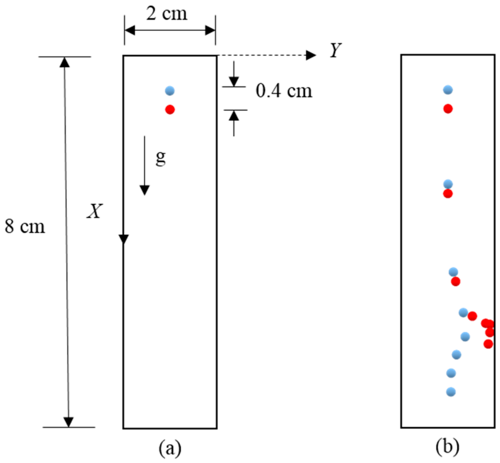
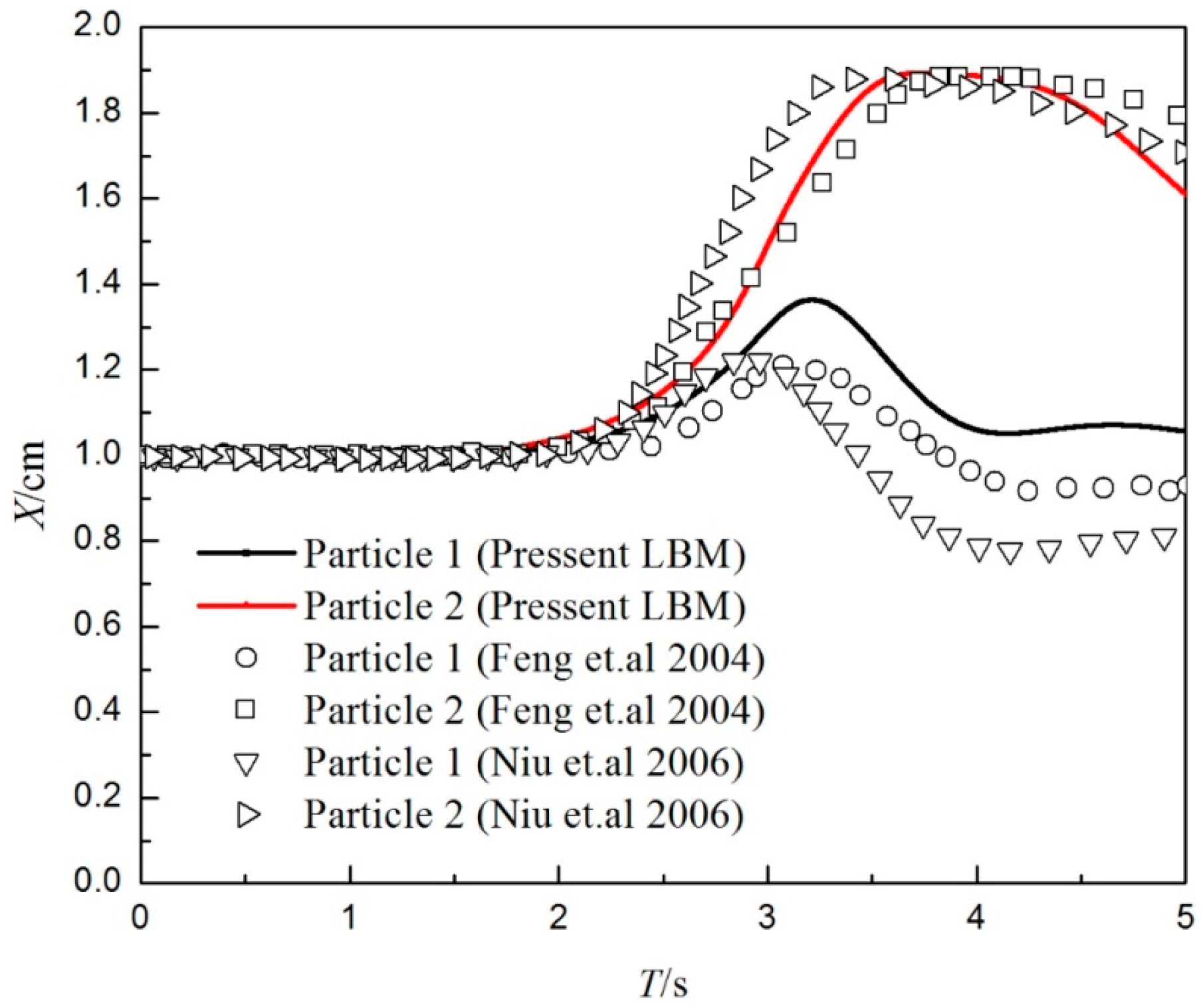
3.2. Two-Particle Sedimentation

For further validating the program, two-particle sedimentation is simulated. The channel geometry is shown in Figure 3a, where the width and length of channel are 2 cm and 8 cm, respectively. The fluid has the properties of water with kinematic viscosity 10⁻⁶ m²/s and density 1000 kg/m³. The diameter of particle is 0.2 cm, and particles density is 1010 kg/m³. The first particle is at 0.999 cm and 0.8 cm in Y and X direction, respectively. The second particle is at 1.0 cm and 1.2 cm in Y and X direction, respectively. For comparison, all these parameters are the same as those in [46,47]. Initially, the two particles are released with a zero velocity, and the upper one will settle in the wake of the other, which leads to the rearrangement mechanism called “drafting, kissing, and tumbling” or DKT motion [48]. Drafting means the particle in the wake will accelerate with an increasing acceleration owing to the low pressure in the wake. Then two particles contact with each other, which is called kissing. Due to the instability of contacting particles aligned in the direction parallel to the motion, they tend to “tumble” to another position. As a result, the center line of particles rotates an angle, and eventually the two particles depart from each other due to the unsymmetrical wake [48].

As show in Figure 3b, our result captures the rearrangement mechanism of “drafting, kissing and tumbling”. Furthermore, the quantitative comparison of particle trajectories in Y direction is presented in Figure 4, which shows that before particles collision our result agree well with that in [46,47]. After kissing stage, exact agreement may not be expected due to different discrete methods are used [47].

4. Numerical Results and Discussion

This section is the main part of this paper. Firstly, the biaxial compression test is simulated to validate the contact bond model and show the influence of bonding strength on macroscopic mechanical behavior of cemented granular media. Then the sand production of cemented granular media is simulated, and the influences of bonding strength and flow rate on sand production are discussed.

The main aim of this work is to investigate the importance of often ignored bonding effect on sand production in previous work. For simplicity and clarity, we treat the porous structure as a hexagonal packing with monodisperse spheres to highlight the bonding effect between particles without the influence of packing way and particle size distribution. In future work, we will refine the porous structure with more realistic sand grains, including the effect of the particle size distribution [25] and non-spherical particles such as polyhedron [49].

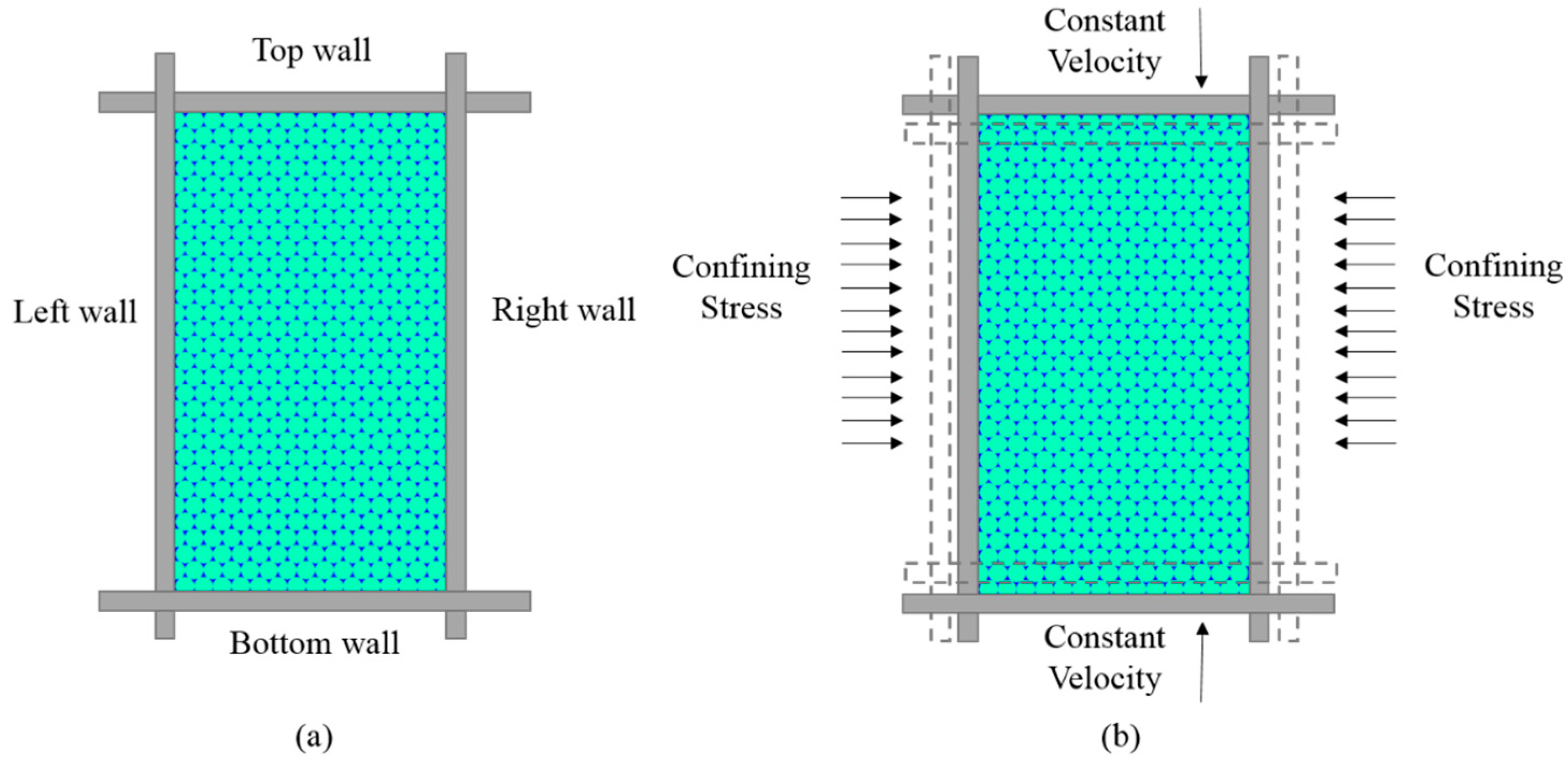
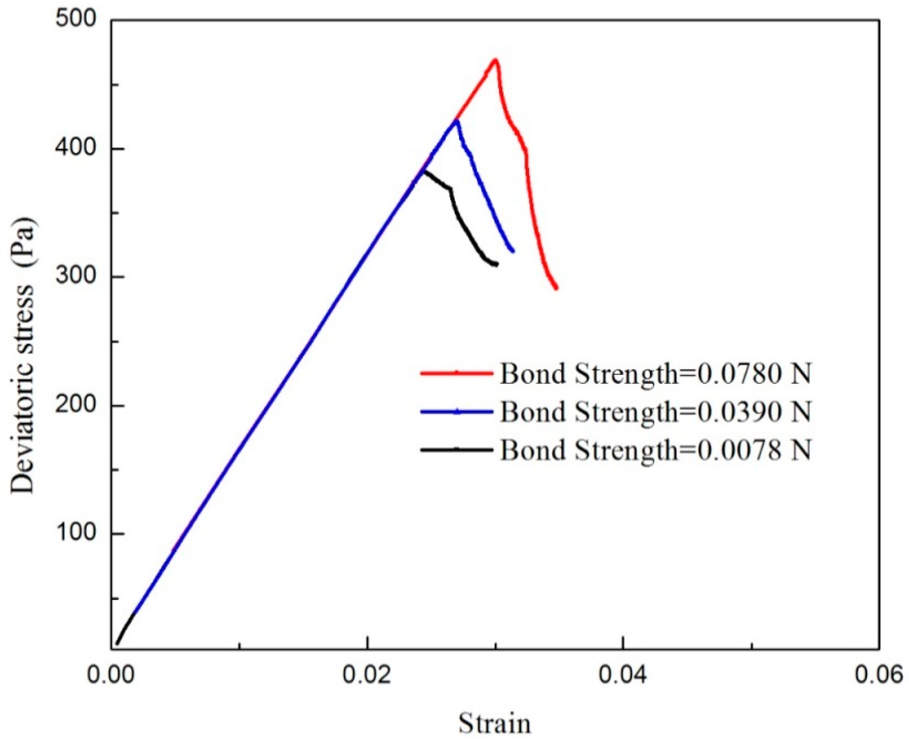
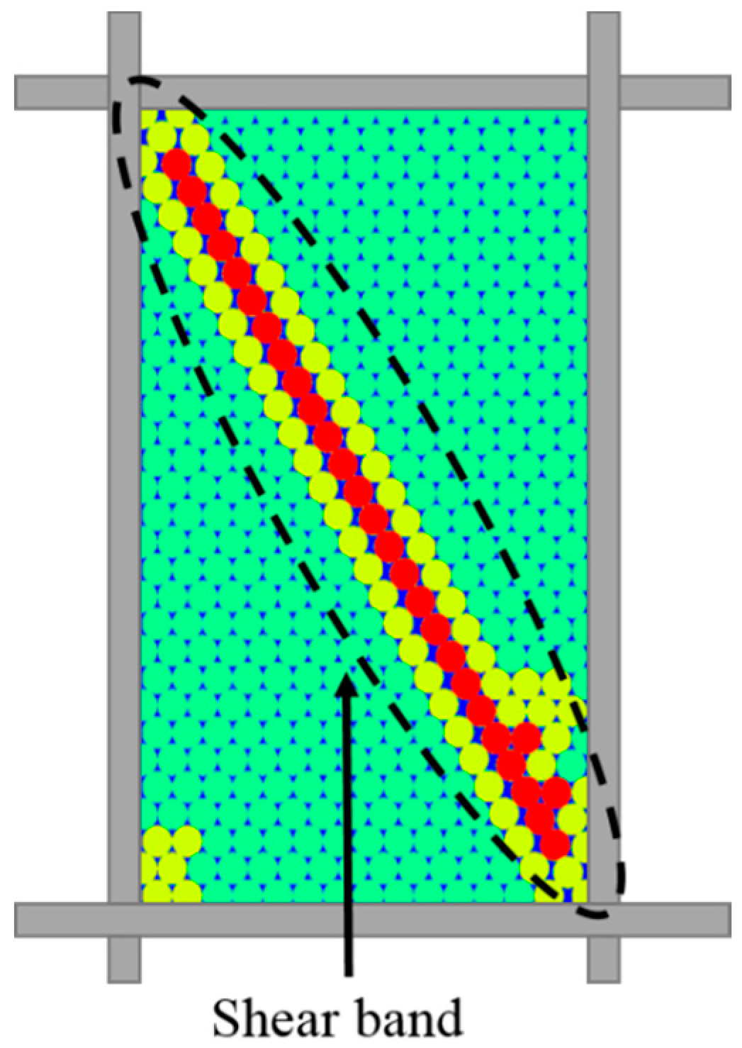
4.1. Biaxial Compression Simulation

Although the bonding effect on macroscopic mechanical behavior of cemented granular media is complex, some general features can still be observed by compression test. These effects include that in cemented materials the macroscopic strength is enhanced and shear band is more likely to be observed [50]. In order to validate the contact bond model and show the influence of bonding strength on macroscopic mechanical behavior, biaxial compression is simulated to capture these effects. The main steps in biaxial compression simulation are sample generation, installing specified isotropic stress and compression.

Firstly, the rectangular DEM samples are bounded by four frictionless rigid walls as in Figure 5a. For capturing the bonding effect in cemented granular media, the contact bond model is added to the particles contacting with each other. In the simulation, three samples are considered, which have the same micro parameters except bonding strength. Due to the limitations of pressure differences that can be applied when using LBM, the samples used in the biaxial compression simulation and sand production simulation have a higher deformability and smaller strength than the real materials, which is a common consideration on simulating sand production by LBM-DEM model [23]. Based on this principal, the main DEM parameters used in biaxial compression and sand production simulation are chosen empirically and summarized in

Table 1. The main parameters used in discrete element method (DEM).

Parameter	Value
Number of particle	600
Diameter of particle	2 mm
$k_n$	2.5 × 104 N/m
$k_s$	1.0 × 104 N/m
μ	0.2
Low bonding strength	0.0078 N
Middle bonding strength	0.039 N
High bonding strength	0.078 N

.

After sample generation, the specimen is isotropically compacted by four walls to reach the isotropic state of stress. Then the biaxial compression is carried out, where the top and bottom walls are moved inward as strain loading condition, and the left and right walls are allowed to displace to retain the confining stress as 111 Pa. In the simulation, the velocity of loading wall is set to a small enough value to ensure a quasi-static process.

Figure 6 shows the deviatoric stress–strain responses of cemented granular media with different bonding strength. It is observed that the synthetic cemented granular media presents a brittle behavior, and the higher the bonding strength is, the more the macroscopic strength is enhanced, which is compatible with the experimental finding in [50]. In addition, the shear band is captured in the biaxial compression simulation as in Figure 7. Therefore our model successfully captures the main features of cemented granular media, and it can be used for a further study.

In cemented granular media, bond is a primary property determining its macroscopic behavior, and the failure of granular media is generally owing to the bond breakage [24]. Thus the number of cumulative bond breakage is monitored during the biaxial compression simulation to show the relationship between bond breakage and macroscopic mechanical behavior. Figure 8 presents the number of accumulative bond during the biaxial compression simulation. It is observed that when the failure of sample occurs, the number of cumulative bond breakage increases greatly, just as in [51]. Thus, in sand production simulation, the number of accumulative bond breakage will be monitored as an indicator of the damage in the sample, and the larger the number is, the closer the sample is to macroscopic failure.

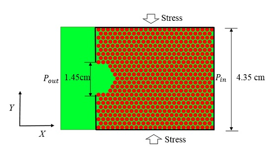
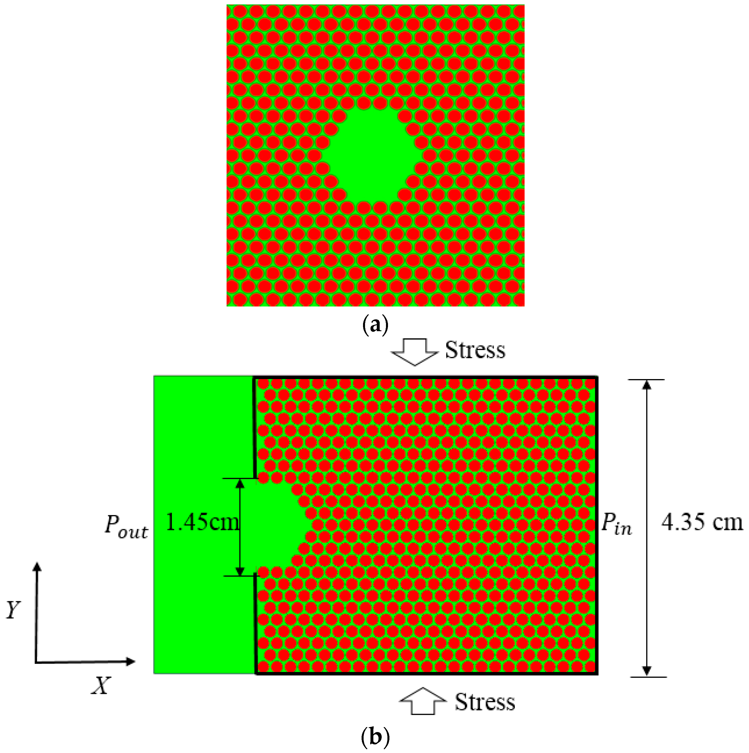
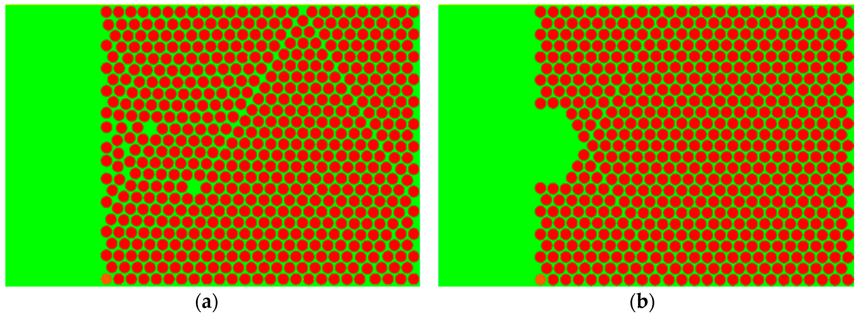
4.2. Sand Production Simulation

Sand production is a phenomenon occurring during the extrusion of hydrocarbons from reservoirs, which makes a lot of trouble on the oil or gas production. Just as discussed above, the behavior of natural sands evidently is distinct from clean sands usually employed in laboratory owing to the influence of bond between sand grains [25]. Therefore, sand production of cemented granular media is simulated in this part by LBM-DEM with contact bond model, and the influences of bonding strength and flow rate on sand production are discussed.

4.2.1. Physical Model

A cross section of a single perforation through a weakly cemented reservoir is shown in Figure 9a. Owing to the high computational costs, it is difficult to consider the whole cross section. Thus the right part of the cross section is isolated to consider the flow erosion and stress loading on matrix, just as in Figure 9b.

The sample is generated by hexagonal packing as in biaxial compression simulation, and for ensuring fluid connectivity in two dimensions, the hydraulic radius is used, which is a common method to deal with flow in two dimensions [7]. In three-dimensionally hexagonal packing of monodisperse sphere, the pore space is one third of the particle radius. In order to ensure the pore space in 2D close to that value, the hydraulic radius of the solid particle is take as 85% the mechanical radius. The cavity in the left part of cemented sample represents the tunnel perforation, which is 1.45 cm, and the rectangular container is created to collect the sand grains eroded by flow. In the following simulation, the dimensionless relaxation time (τ) is equal to 1, and there are 1396 lattices in Y direction leading to the grid size at 1.116 × 10⁻⁵ m. From Equation (2) the time step can be calculated (dt = 1.6 × 10⁻⁴ s) which is a safe value for a stable solution in DEM integration, because it is smaller than the DEM critical time step limit (9 × 10⁻⁴ s) calculated by:

$$d{t}_{DEM}^{cri}=\sqrt{m/K_n}$$

where m is the mass of particle, K_n is the normal spring stiffness. Moreover, under this grid system the largest Mach number in sand production simulation is O(10⁻³) which is much smaller than 0.1, so the deleterious compressibility effect can be annihilated [15].

In order to couple the two mechanisms in sand production: (i) mechanical instabilities and (ii) hydro-mechanical instabilities [6], an external stress is loaded in Y direction and a fluid flow is applied in X direction. Thus the top and bottom wall are moved inwards as a stress loading in Y direction with the left and right wall fixed. During the simulation the strain in y direction is monitored to reflect loading condition. Meanwhile, the fluid with the property of water is set a pressure drop in X direction to capture the flow erosion, and in Y direction the top and bottom wall are treated as no-slip boundary condition.

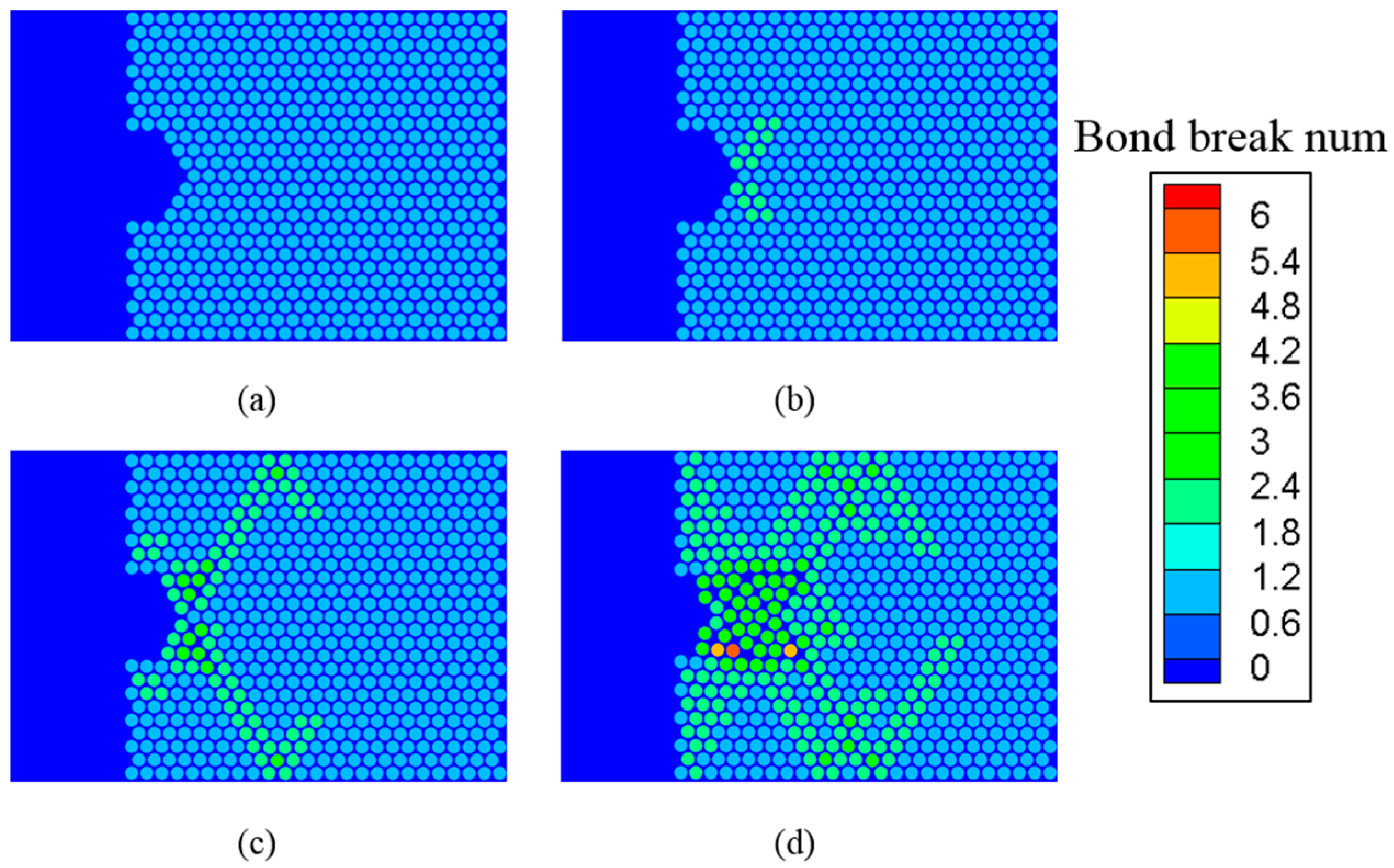
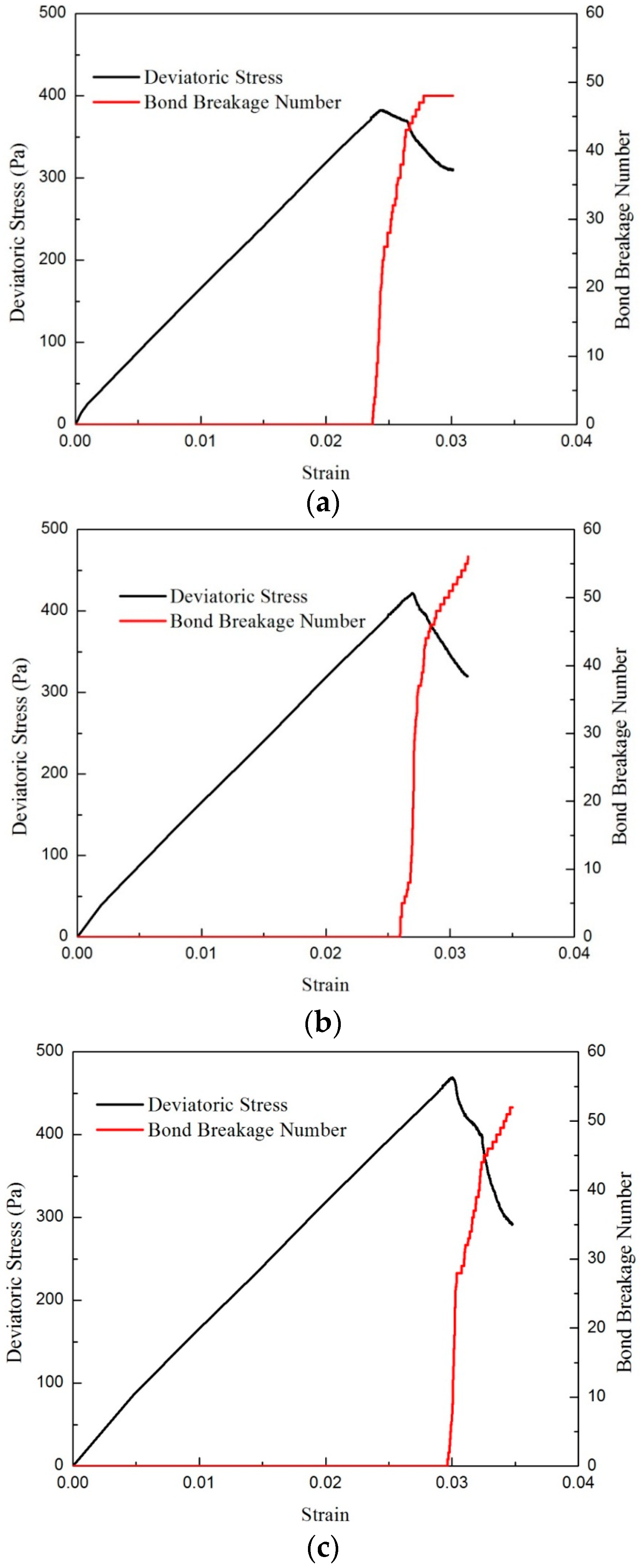
4.2.2. Damage Evolution

Before quantitative discussion, the phenomenological observation of damage evolution in cemented granular media is presented firstly to understand the process of sand production, which is important to study the instability mechanism on sand production [5]. Although visualization is quite cumbersome in experiment, it can be easily achieved using simulations (Figure 10).

Figure 10 shows the damage evolution of the cemented sample with bonding strength of 0.078 N under the effective stress and flow erosion, where the color of the sand grain represents the number of bond breakage, and the warmer the color is, the more bonds on the sand grain are broken. Initially, the sample is intact with no bonding breakage (Figure 10a). With the increase of the strain, the bond near the cavity begins to be broken owing to the concentration of effective stress, and some small cracks forms in this zone (Figure 10b). Then, these small cracks propagate into the sample, which leads to the localized failure near the cavity (Figure 10c). Eventually, the flow erodes the localized failure zone and transfers the loose sand grains into the cavity (Figure 10d). It is observed that the experimental observation “initial sand production is evoked by localized failure” in [5] is examined by our simulation. What is more, although the localized failure is serious near the cavity, the zone far from the cavity is still intact, which means that sand production occurs well before macroscopic failure, just as the experimental observation by X-ray CT photographs in [5].

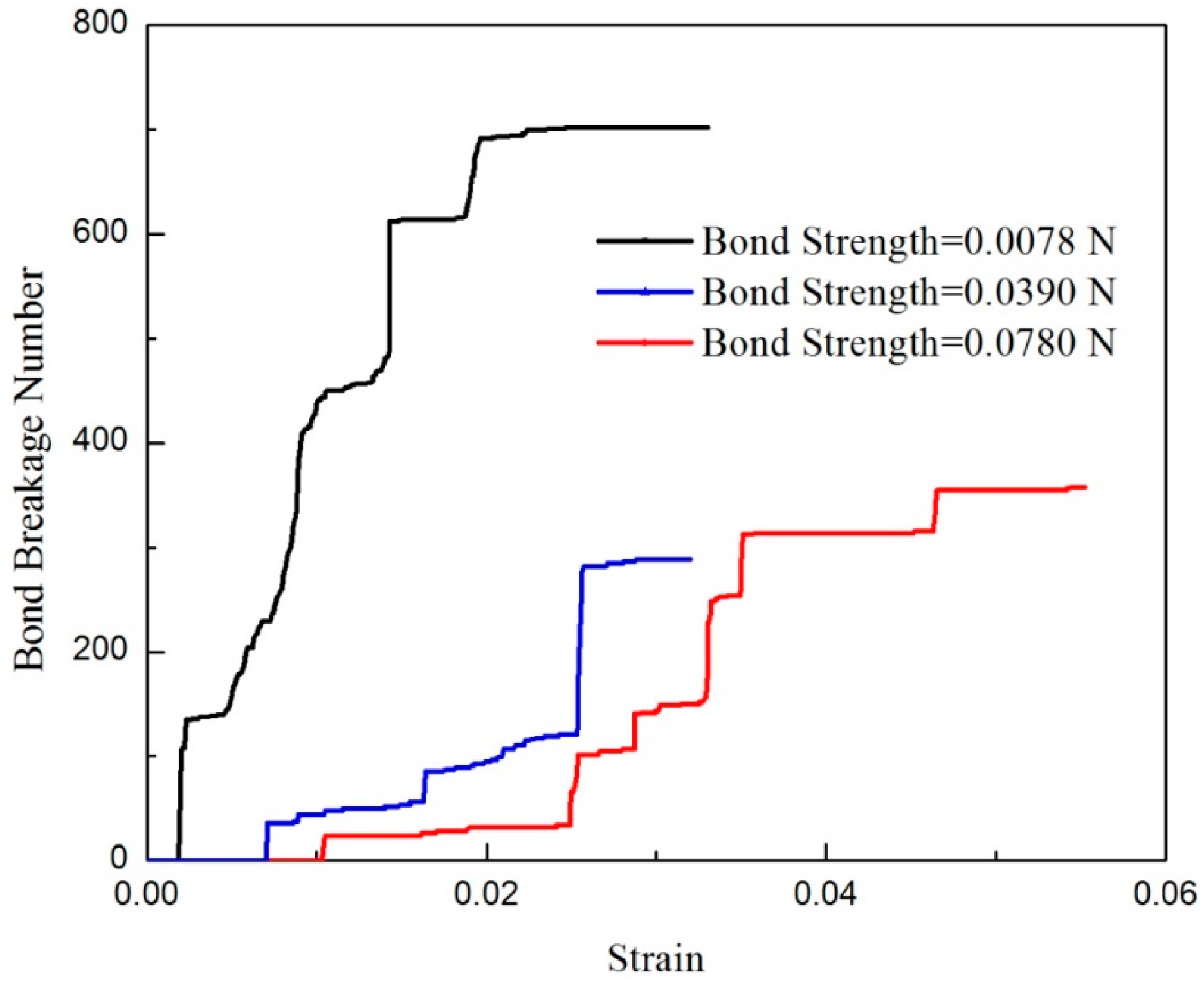
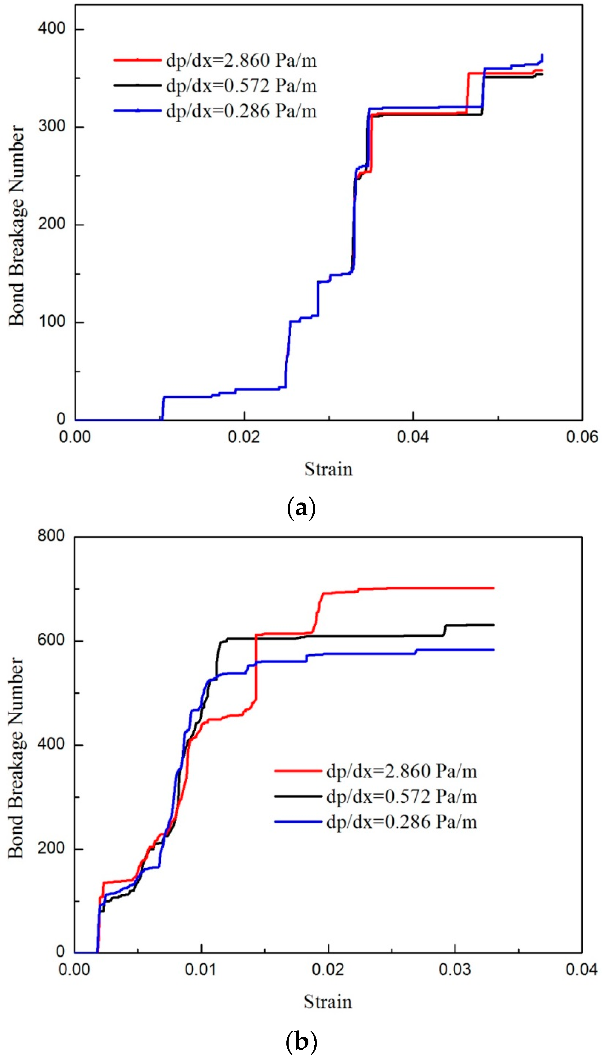
4.2.3. Effect of Bonding Strength

In cemented granular media, bonding strength is a primary property that influences its mechanical behavior. It is necessary to study the effect of bonding strength on sand production, so three cemented samples with different bonding strength are considered, which are 0.0078 N, 0.039 N and 0.078 N, respectively. Just as illustrated above, during sand production simulation the accumulative bond breakage is monitored as an indicator of the damage caused by effective stress and flow erosion.

Figure 11 shows the number of accumulative bond breakage in three samples under the same flow condition (dp/dx = 2.86 Pa/m). First, a staged growth of accumulative bond breakage is observed for all samples, which means a great increase of bond breakage is always followed by a very slow growth. This is owing to the fact that under effective stress and flow erosion, instability and temporary stability take place alternately in cemented sample. Before macroscopic failure, the cemented granular media is in a temporarily stable state until the effective stress increases to a value strong enough to break this temporarily stable state. Because the macroscopic failure has not occurred, another temporarily stable state can be rebuilt. As a result, on the temporarily stable state, a few bonds are broken in the sample, but when the temporarily stable state is broken, a great increase of bond breakage can be observed. These two states occurring alternately lead to the staged growth of accumulative bond breakage (Figure 11).

Although the tendencies of three curves are same, some obvious differences are still observed in Figure 11. First, the bond breakage occurs until the strain reaches a critical point, and higher bonding strength sample corresponds to a higher critical strain. This is because, for intact sample, the seepage force is too weak to break the bond, and the initial bond breakage is evoked by the concentration of effective stress near the cavity. Thus only beyond the critical strain, the effective stress is strong enough to break the bond, and the higher the bonding strength is, the higher effective stress is needed to break it. As a result, higher bonding strength leads to a higher critical strain to evoke the initial bond breakage. Another significant difference in Figure 11 is that under the same strain and flow condition, the accumulative bond breakage in low bonding strength sample is much greater than that in high bonding strength sample. Therefore, the cemented material with lower bonding strength is more likely to produce sand grains, which is confirmed in Figure 12. Figure 12 shows the states of two cemented samples with different bonding strength (0.0078 N and 0.078 N) under the same strain (0.024) and flow condition (dp/dx = 2.86 Pa/m). For higher bonding strength sample, as in Figure 12b, the cavity is stable, and no sand grains are produced. However, for lower bonding strength sample, as in Figure 12a, the stability of cavity is broken, and sand production continues up to end of the simulation. Therefore, for samples under the same condition, lower bonding strength leads to more sand production than higher bonding strength.

4.2.4. The Effect of Flow Rate

Flow rate is the other important factor that influences the process of sand production in cemented reservoir, which leads to the hydro-mechanical instability. In the simulation, three kinds of pressure gradient are considered to study the influence of flow rate on sand production, which are 0.286 Pa/m, 0.572 Pa/m and 2.86 Pa/m, respectively.

Figure 13 shows the influence of flow rate on accumulative bond breakage in cemented granular media with bond strength of 0.0078 N and 0.078 N. It is observed that the influence of flow rate becomes significant until the strain reach some critical value, which confirms the conclusion that the role of flow in sand production is to erode the localized failure zone [4,5]. Before the critical strain, the cemented granular media is almost intact, and the hydrodynamic force provided by the highest flow rate cannot erode the sample. Therefore, there is little difference between various pressure gradient conditions. After the critical point, the localized failure near the cavity occurs, and the flow erosion starts to take effects, and the coupling effect of mechanical instability and hydro-mechanical instability becomes significant, so the curves of different flow rates begin to deviate from each other.

Comparing Figure 13a,b, in high bonding strength sample (0.078 N), the accumulative bond breakage under different flow conditions is almost same, but in low bonding strength sample (0.0078 N), the gap between different flow conditions is obvious and higher flow rate leads to more bond breakage. Therefore the influence of flow rate on sand production depends on the bonding strength, and it is more significant in lower bonding strength sample than in higher bonding strength sample. The same result was also obtained in [5], that the effect of flow rate on weak rock is in contrast to that on more competent rock. In competent rock, the localized failure zone is hard to be eroded by flow owing to the residual bond with high strength, so the coupling effect between mechanical instability and hydro-mechanical instability is not significant. However, in weak rock, the localized failure zone is easily eroded, which leads to a significant coupling effect between mechanical instability and hydro-chemical instability, so the influence of flow rate on sand production is more obvious in lower bonding strength sample.

5. Conclusions

In this study, the sand production in cemented reservoir is simulated at pore scale by LBM-DEM. In order to account for the bonding effect in cemented granular media, a contact bond model is introduced into the LBM-DEM framework, which is validated by benchmark cases. By sand production simulation, the experimental observation that “initial sand production is evoked by localized failure” is confirmed, and it is also found that instability and temporary stability take place alternately in cemented granular media, until the macroscopic failure occurs. Then the influence of bonding strength on sand production is discussed. Under the same condition, the cemented granular media with low bonding strength is easier to produce sand than that with high bonding strength. Finally, the effect of flow rate is invested, and it illustrates that the influence of flow rate on sand production depends on the bonding strength. In higher bonding strength sample, the influence of flow rate on sand production is not significant. However, in low bonding strength sample, the higher the flow rate is, the more severe the erosion in localized failure zone becomes. Therefore, this simulation captures the main feature of sand production in cemented reservoir and discusses the influence of the micro parameters, which helps us understand the underlying physics of this problem at pore scale. Since only 2D simulations are performed in this paper, in the future we will consider 3D simulations and enlarge our computational scale to make it more suitable for actual situation.

References

1. Ranjith, P.G.; Perera, M.S.A.; Perera, W.K.G.; Wu, B.; Choi, K.S. Effective parameters for sand production in unconsolidated formations: An experimentl study. J. Petrol. Sci. Eng. 2013, 105, 34–42. [Google Scholar] [CrossRef]
2. Papamichos, E. Erosion and multiphase flow in porous media: Application to sand production. Eur. J. Environ. Civ. Eng. 2010, 14, 1129–1154. [Google Scholar] [CrossRef]
3. Ranjith, P.G.; Pereraa, M.S.A.; Pereraa, W.K.G.; Choib, S.K.; Yasarc, E. Sand production during the extrusion of hydrocarbons from geological formations: A review. J. Petrol. Sci. Eng. 2014, 124, 72–82. [Google Scholar] [CrossRef]
4. Van den Hoek, P.; Hertogh, G.M.M.; Kooijman, A.P.; de Bree, P.; Kenter, C.J.; Papamichos, E. A new concept of sand production prediction: Theory and laboratory experiments. SPE Drill. Complet. 2000, 15, 261–273. [Google Scholar] [CrossRef]
5. Tronvoll, J.; Skj, A.; Papamichos, E. Sand production: Mechanical failure or hydrodynamic erosion? Int. J. Rock Mech. Min. Sci. 1997, 34, 291. [Google Scholar] [CrossRef]
6. Vardoulakis, I.; Stavropoulou, M.; Papanastasiou, P. Hydro-mechanical aspects of the sand production problem. Transp. Porous Med. 1996, 22, 225–244. [Google Scholar] [CrossRef]
7. Boutt, D.F.; Cook, B.K.; Williams, J.R. A coupled fluid-solid model for problems in geomechanics: Application to sand production. Int. J. Numer. Anal. Methods Geomech. 2011, 35, 997–1018. [Google Scholar] [CrossRef]
8. Cundall, P.A.; Strack, O.D. A discrete numerical model for granular assemblies. Geotechnique 1979, 29, 47–65. [Google Scholar] [CrossRef]
9. O’Connor, R.M.; Torczynski, J.R.; Preece, D.S.; Klosek, J.T.; Williams, J.R. Discrete element modeling of sand production. Int. J. Rock Mech. Min. Sci. Geomech. Abstr. 1997, 34, 231. [Google Scholar] [CrossRef]
10. Jensen, R.P.; Preece, D.S. Modeling Sand Production with Darcy-Flow Coupled with Discrete Elements; Sandia National Labs: Albuquerque, NM, USA; Livermore, CA, USA, 2000.
11. Zhou, Z.Y.; Yu, A.B.; Choi, S.K. Numerical simulation of the liquid-induced erosion in a weakly bonded sand assembly. Powder Technol. 2011, 211, 237–249. [Google Scholar] [CrossRef]
12. Climent, N.; Arroyoa, M.; O’Sullivanb, C.; Gensa, A. Sand production simulation coupling DEM with CFD. Eur. J. Environ. Civ. Eng. 2014, 18, 983–1008. [Google Scholar] [CrossRef]
13. Li, L.; Papamichos, E.; Cerasi, P. Investigation of sand production mechanisms using DEM with fluid flow. In Proceedings of the International Symposium of the International Society for Rock Mechanics (Eurock’06), Liege, Belgium, 13–15 August 2014.
14. Han, Y.; Cundall, P.A. LBM-DEM modeling of fluid-solid interaction in porous media. Int. J. Numer. Anal. Methods Geomech. 2013, 37, 1391–1407. [Google Scholar] [CrossRef]
15. Chen, S.; Doolen, G.D. Lattice boltzmann method for fluid flows. Annu. Rev. Fluid Mech. 1998, 30, 329–364. [Google Scholar] [CrossRef]
16. Wang, M.; Chen, S. Electroosmosis in homogeneously charged micro- and nanoscale random porous media. J. Coll. Interface Sci. 2007, 314, 264–273. [Google Scholar] [CrossRef] [PubMed]
17. Wang, M.; Pan, N. Predictions of effective physical properties of complex multiphase materials. Mater. Sci. Eng. R Rep. 2008, 63, 1–30. [Google Scholar] [CrossRef]
18. Aidun, C.K.; Clausen, J.R. Lattice-Boltzmann Method for Complex Flows. Annu. Rev. Fluid Mech. 2010, 42, 439–472. [Google Scholar] [CrossRef]
19. Ladd, A.J.C. Numerical simulations of particulate suspensions via a discretized Boltzmann equation. Part 1. Theoretical foundation. J. Fluid Mech. 1994, 271, 285–309. [Google Scholar] [CrossRef]
20. Aidun, C.K.; Lu, Y.; Ding, E.J. Direct analysis of particulate suspensions with inertia using the discrete Boltzmann equation. J. Fluid Mech. 1998, 373, 287–311. [Google Scholar] [CrossRef]
21. Chen, Y.; Kanga, Q.; Caia, Q.; Wanga, M.; Zhang, D. Lattice Boltzmann Simulation of Particle Motion in Binary Immiscible Fluids. Commun. Comput. Phys. 2015, 18, 757–786. [Google Scholar] [CrossRef]
22. Ghassemi, A.; Pak, A. Numerical simulation of sand production experiment using a coupled Lattice Boltzmann-Discrete Element Method. J. Petrol. Sci. Eng. 2015, 135, 218–231. [Google Scholar] [CrossRef]
23. Velloso, R.Q.; Vargas, E.A.; Goncalves, C.J.; Prestes, A. Analysis of sand production processes at the pore scale using the discrete element method and lattice Boltzman procedures. In Proceedings of the 44th US Rock Mechanics Symposium and 5th US-Canada Rock Mechanics Symposium, Salt Lake City, UT, USA, 27–30 June 2010.
24. Tronvoll, J.; Papamichos, E.; Skjaerstein, A.; Sanfilippo, F. Sand production in ultra-weak sandstones: Is sand control absolutely necessary? In Proceedings of the Latin American and Caribbean Petroleum Engineering Conference, Rio de Janeiro, Brazil, 30 August–3 September 1997.
25. Jiang, M.; Yu, H.S.; Leroueil, S. A simple and efficient approach to capturing bonding effect in naturally microstructured sands by discrete element method. Int. J. Numer. Methods Eng. 2007, 69, 1158–1193. [Google Scholar] [CrossRef]
26. Servant, G.; Marchina, P.; Nauroy, J.F. Near Wellbore Modeling: Sand Production Issues. In Proceedings of the SPE Annual Technical Conference and Exhibition, Anaheim, CA, USA, 11–14 November 2007.
27. Wang, M.; Kang, Q.J.; Pan, N. Thermal conductivity enhancement of carbon fiber composites. Appl. Ther. Eng. 2009, 29, 418–421. [Google Scholar] [CrossRef]
28. Wang, M.; Pan, N.; Wang, J.; Chen, S. Lattice Poisson-Boltzmann simulations of electroosmotic flows in charged anisotropic porous media. Commun. Comput. Phys. 2007, 2, 1055–1070. [Google Scholar]
29. Wang, M.; Kang, Q.; Viswanathan, H.; Robinson, B. Modeling of electro-osmosis of dilute electrolyte solutions in silica microporous media. J. Geophys. Res. Solid Earth 2010, 115. [Google Scholar] [CrossRef]
30. Wang, M.R.; Kang, Q.J. Electrokinetic Transport in Microchannels with Random Roughness. Anal. Chem. 2009, 81, 2953–2961. [Google Scholar] [CrossRef] [PubMed]
31. Zhang, L.; Wang, M.R. Modeling of electrokinetic reactive transport in micropore using a coupled lattice Boltzmann method. J. Geophys. Res. Solid Earth 2015, 120, 2877–2890. [Google Scholar] [CrossRef]
32. Yang, X.; Mehmanib, Y.; Perkinsa, W.A.; Pasqualic, A.; Schönherrc, M.; Kimd, K.; Peregod, M.; Parksd, M.L.; Traske, N.; Balhoff, M.T. Intercomparison of 3D pore-scale flow and solute transport simulation methods. Adv. Water Resour. 2015. [Google Scholar] [CrossRef]
33. Kang, Q.J.; Zhang, D.X.; Chen, S.Y. Displacement of a two-dimensional immiscible droplet in a channel. Phys. Fluids 2002, 14, 3203–3214. [Google Scholar] [CrossRef]
34. Huang, H.B.; Lu, X.Y. Relative permeabilities and coupling effects in steady-state gas-liquid flow in porous media: A lattice Boltzmann study. Phys. Fluids 2009, 21, 092104. [Google Scholar] [CrossRef]
35. Huang, H.B.; Wang, L.; Lu, X.Y. Evaluation of three lattice Boltzmann models for multiphase flows in porous media. Comput. Math. Appl. 2010, 61, 3606–3617. [Google Scholar] [CrossRef]
36. Huang, H.B.; Huang, J.J.; Lu, X.Y. Study of immiscible displacements in porous media using a color-gradient-based multiphase lattice Boltzmann method. Comput. Fluids 2014, 93, 164–172. [Google Scholar] [CrossRef]
37. Chen, L.; Kang, Q.; Mu, Y.; He, Y.; Tao, W. A critical review of the pseudopotential multiphase lattice Boltzmann model: Methods and applications. Int. J. Heat Mass Transf. 2014, 76, 210–236. [Google Scholar] [CrossRef]
38. Chen, Y.; Cai, Q.; Xia, Z.; Wang, M.; Chen, S. Momentum-exchange method in lattice Boltzmann simulations of particle-fluid interactions. Phys. Rev. E Stat. Nonlinear Soft Matter Phys. 2013, 88, 013303. [Google Scholar] [CrossRef] [PubMed]
39. De Rosis, A. On the dynamics of a tandem of asynchronous flapping wings: Lattice Boltzmann-immersed boundary simulations. Phys. A Stat. Mech. Appl. 2014, 410, 276–286. [Google Scholar] [CrossRef]
40. Cao, C.; Chen, S.; Li, J.; Liu, Z.; Zha, L.; Bao, S.; Zheng, C. Simulating the interactions of two freely settling spherical particles in Newtonian fluid using lattice-Boltzmann method. Appl. Math. Comput. 2015, 250, 533–551. [Google Scholar] [CrossRef]
41. Galindo-Torres, S. A coupled Discrete Element Lattice Boltzmann Method for the simulation of fluid-solid interaction with particles of general shapes. Comput. Methods Appl. Mech. Eng. 2013, 265, 107–119. [Google Scholar] [CrossRef]
42. Verlet, L. Computer “experiments” on classical fluids. I. Thermodynamical properties of Lennard-Jones molecules. Phys. Rev. 1967, 159, 98. [Google Scholar] [CrossRef]
43. Jiang, M.; Yan, H.B.; Zhu, H.H.; Utili, S. Modeling shear behavior and strain localization in cemented sands by two-dimensional distinct element method analyses. Comput. Geotech. 2011, 38, 14–29. [Google Scholar] [CrossRef]
44. Wen, B.; Li, H.; Zhang, C.; Fang, H. Lattice-type-dependent momentum-exchange method for moving boundaries. Phys. Rev. E 2012, 85, 016704. [Google Scholar] [CrossRef] [PubMed]
45. Feng, J.; Hu, H.H.; Joseph, D.D. Direct simulation of initial value problems for the motion of solid bodies in a Newtonian fluid Part 1. Sedimentation. J. Fluid Mech. 1994, 261, 95–134. [Google Scholar] [CrossRef]
46. Feng, Z.G.; Michaelides, E.E. The immersed boundary-lattice Boltzmann method for solving fluid-particles interaction problems. J. Comput. Phys. 2004, 195, 602–628. [Google Scholar] [CrossRef]
47. Niu, X.D.; Shu, C.; Chew, Y.T.; Peng, Y. A momentum exchange-based immersed boundary-lattice Boltzmann method for simulating incompressible viscous flows. Phys. Lett. Sect. A Gen. Atom. Solid State Phys. 2006, 354, 173–182. [Google Scholar] [CrossRef]
48. Fortes, A.F.; Joseph, D.D.; Lundgren, T.S. Nonlinear mechanics of fluidization of beds of spherical particles. J. Fluid Mech. 1987, 177, 467–483. [Google Scholar] [CrossRef]
49. Galindo-Torres, S.; Pedroso, D.M.; Williams, D.J.; Mühlhaus, H.B. Strength of non-spherical particles with anisotropic geometries under triaxial and shearing loading configurations. Granul. Matter 2013, 15, 531–542. [Google Scholar] [CrossRef]
50. Wang, Y.H.; Leung, S.C. A particulate-scale investigation of cemented sand behavior. Can. Geotech. J. 2008, 45, 29–44. [Google Scholar] [CrossRef]
51. Hazzard, J.F.; Young, R.P.; Maxwell, S. Micromechanical modeling of cracking and failure in brittle rocks. J. Geophys. Res. Solid Earth 2000, 105, 16683–16697. [Google Scholar] [CrossRef]
Figure 1. The computation of lattice Boltzmann method (LBM) and discrete element method (DEM) coupling.
Computation 04 00015 g001
Figure 2. The benchmark case of single particle sedimentation. (a) The geometry of the simulation; (b) the comparison of particle trajectories.
Computation 04 00015 g002
Figure 3. The benchmark case of two particles sedimentation. (a) The geometry of the simulation; (b) the settling trajectory of two-particle sedimentation.
Computation 04 00015 g003
Figure 4. Transverse coordinates of the centers of the two particles.
Computation 04 00015 g004
Figure 5. The DEM sample for biaxial compression simulation. (a) The hexagonal packing of the granular media; (b) the boundary condition for biaxial compression simulation.
Computation 04 00015 g005
Figure 6. The deviatoric stress–strain responses of cemented granular media in biaxial compression simulation.
Computation 04 00015 g006
Figure 7. Shear band after macroscopic failure of cemented granular media in the biaxial compression simulation.
Computation 04 00015 g007
Figure 8. The deviatoric stress–strain response and number of accumulative bond breakage during biaxial compression: (a) bonding strength is 0.0078 N; (b) bonding strength is 0.039 N; and (c) bonding strength is 0.078 N.
Computation 04 00015 g008
Figure 9. The cemented granular media used in sand production simulation. (a) The cross section of a single perforation in cemented reservoir; (b) the geometry of sample used in sand production simulation.
Computation 04 00015 g009
Figure 10. The process of sand production in cemented granular media. (a) Initially, the sample is intact with no bonding breakage; (b) the bond near the cavity begins to be broken; (c) small cracks propagate into the sample leading to the localized failure near the cavity; (d) the flow erodes the localized failure zone.
Computation 04 00015 g010
Figure 11. The number of accumulative bond breakage for three cemented samples under the pressure gradient of 2.86 Pa/m.
Computation 04 00015 g011
Figure 12. The state of cemented granular media with different bond strengths under the same effective stress and flow erosion: (a) continuous sand production for low bonding strength 0.0078 N; and (b) the stable cavity for high bonding strength 0.078 N.
Computation 04 00015 g012
Figure 13. The number of accumulative bond breakage for synthetic cemented materials: (a) with high bonding strength 0.078 N; and (b) with low bonding strength 0.0078 N under different flow rate.
Computation 04 00015 g013