Stochastic Semantic Fields for Sentiment-Driven Models

Abstract

This article studies a time-dependent latent sentiment representation governed by a semilinear stochastic evolution equation on a separable Hilbert space. The objective is to derive uncertainty, interpretability, and robustness from one stochastic law. The mathematical analysis establishes covariance propagation and spectral uncertainty attribution, Fréchet differentiability of the forcing-to-state and forcing-to-readout maps with quadratic remainders, trace-norm differentiation of the covariance, and an adjoint influence kernel whose norm equals the exact worst-case displacement over an energy-bounded forcing ball in the linear regime. The dependence of the certificates on dissipativity, forecast horizon, noise geometry, and spectral truncation is made explicit. A Galerkin state-space reduction yields exact linear transitions, a likelihood-based calibration scheme, and structural identifiability conditions. A reproducible three-mode study verifies the covariance and duality identities, evaluates the sensitivity constants, and compares Gaussian with split-conformal predictive intervals under controlled synthetic conditions. The results provide a rigorous operator calculus and a tractable finite approximation. They establish internal mathematical and numerical validity without asserting a generalised superiority.

1. Introduction

Contextual encoders and large language models have increased the expressive power of sentiment systems while also making their temporal behaviour harder to analyse. A terminal score may appear accurate even when its dispersion is poorly calibrated, its response to earlier semantic evidence is opaque, or a modest perturbation of the information stream creates a large displacement. The mathematical problem studied here is the construction of uncertainty, interpretability, and robustness from one time-dependent stochastic law. This problem matters whenever sentiment enters a sequential decision process, since the reliability of the terminal output depends on the evolution that produced it.

Classical work established the linguistic and computational foundations of opinion mining [1,2], and transformer encoders supplied a high-dimensional geometry for contextual text representations [3]. Current large language model studies show that strong aggregate performance does not remove weaknesses on structured sentiment phenomena [4]. Progressive task adaptation improves generic affective capabilities [5], while causal analysis reveals that apparently simple sentiment decisions may involve distinct internal reasoning routes [6]. The faithfulness of model-generated explanations remains dependent on the architecture and the task [7]. These findings motivate a dynamical representation in which semantic evidence evolves before the readout is formed and in which the resulting diagnostic quantities have operator-level definitions.

Bayesian approximations and post-training calibration remain central finite-dimensional tools [8,9,10]. Conformal prediction complements them by providing distribution-free marginal coverage under exchangeability [11,12]. Recent evidence also shows that in-context language model probabilities can remain substantially miscalibrated [13]. The present framework uses covariance propagation to describe the internal transport of stochastic uncertainty. The synthetic study then applies split conformal calibration to terminal projected residuals. The covariance operator supplies a structural decomposition, whereas the conformal layer supplies a finite-sample coverage statement for the projected predictor.

Interpretability and robustness are derived from the same solution map. Local surrogate methods and Shapley-type attributions remain influential [14,15], while adversarial analyses have documented the fragility of text systems under constructed and naturally occurring perturbations [16,17,18]. In the present setting, the Fréchet derivative of the terminal readout with respect to the forcing path defines the explanation. Its Riesz representative is an adjoint influence kernel. The norm of this kernel equals the exact worst-case displacement of a linear readout over an energy-bounded forcing ball; consequently, the Hilbert-space duality links interpretability and robustness exactly.

The latent state is modelled in a separable Hilbert space through

$$d{X}_t=\left[A{X}_t+F\left(X_t\right)+B{u}_t\right]dt+G\left(X_t\right)d{W}_t,X_0=x.$$

(1)

A time-indexed text encoder produces the forcing path u. The bounded map B lifts that path into the state space. The generator A propagates information across semantic directions, while F describes state-dependent response, and G transmits unresolved variability. A scalar prediction is obtained from $\mathsf{\Phi }\left(X_T\right)$. When the semantic representation carries a neighbourhood structure, a graph Laplacian or a kernel operator gives a concrete approximation of A. Large eigenvalues then describe coordinates with high Dirichlet energy across neighbouring semantic prototypes. The phrase high semantic frequency refers to this graph-spectral variation and not to token frequency.

The analytic setting follows the semigroup theory of stochastic evolution equations [19,20,21]. Approximation theory for semilinear stochastic evolution equations provides the connection between the infinite-dimensional field and its finite projections [22]. Stochastic reaction-diffusion equations on networks provide a direct precedent for random diffusion over graph-like structures [23]. These two articles by Luca Di Persio and coauthors are pertinent to the Galerkin and network mechanisms used below.

Computational work on stochastic partial differential equations has also moved towards learned solution operators. Neural stochastic PDEs aim at resolution-invariant learning of continuous random dynamics [24]. Regularity-informed architectures and Bayesian deep solvers address stochastic forward and inverse problems while retaining information about numerical uncertainty [25,26]. Such methods can approximate the projected state equation. The operator identities proved here provide independent checks for covariance propagation, adjoint sensitivity, and spectral truncation.

A broader numerical PDE literature clarifies the methodological position of the paper. Dissipative PDE evolution can serve as a denoising mechanism [27]. Deep learning can recover forward solutions and unknown coefficients for coupled nonlinear wave equations [28]. Lie-group methods show how a high-order discretisation can preserve a prescribed invariant [29], while the Riemann–Hilbert method provides exact spectral information for integrable coupled systems [30]. Artificial-intelligence-enhanced mathematical derivation combines learned search with symbolic verification of exact formulae [31]. The stochastic semantic field has a dissipative probabilistic structure. Its numerical approximations must therefore preserve contractivity, covariance positivity, and consistency between the forward and adjoint equations. The cited methods supply complementary inverse, geometric, spectral, and symbolic techniques. Their mathematical targets differ from the sentiment model.

Appendix A contains the stochastic-convolution estimates, the fixed-point existence proof, finite-horizon input stability, fourth-moment estimates, Galerkin consistency, covariance identities, and the Yosida passage used in the main proofs. Theorem 1 and Theorem 13 adapt established synchronous-coupling and Gronwall arguments to the semantic-field setting. The model-specific contribution begins with the joint covariance, sensitivity, and perturbation calculus. It includes a genuine Fréchet differentiability theorem with a quadratic remainder, trace-norm differentiation of covariance, an adjoint influence representation, exact influence-robustness duality, and explicit truncation and ablation formulae.

The computational part uses a reproducible three-mode Galerkin experiment. In particular, exact transitions are used to estimate a stable state-space model, to compare it with finite-dimensional baselines, evaluate Gaussian and split-conformal intervals, and verify the covariance and duality identities. The experiment also measures the dependence of the diagnostics on dissipation and noise geometry. It establishes internal numerical validity under controlled synthetic conditions. Sentiment140, SemEval, TweetEval, IMDb, and the NRC Emotion Lexicon are discussed as candidate resources for a subsequent study [32,33,34,35,36].

Section 2 develops the analytical results and their proofs. Section 3 gives the finite-dimensional calibration map. Section 4 presents the synthetic study. Section 5 states the conclusions and the scope of the claims. The appendices contain the standard analytical material and the conformal coverage argument.

2. Original Theoretical Contributions and Proofs

The analytical architecture separates classical stochastic-evolution theory from the results that are specific to sentiment-driven diagnostics. Appendix A supplies the existence theory and the approximation devices required to manipulate mild solutions. The contraction theorem below and the later finite-horizon perturbation theorem adapt standard Hilbert-space stability arguments to the semantic field notation and make the dependence on the dissipativity and Lipschitz constants explicit. The original contribution lies in the joint operator calculus built on top of that state equation. The covariance of the latent field is pushed to an output uncertainty and decomposed spectrally. The solution map with respect to semantic forcing is differentiated in the Fréchet sense with a uniform quadratic remainder. This derivative yields a trace-norm covariance derivative and an adjoint influence kernel. The kernel norm is proved to equal the exact worst-case displacement over an input energy ball. Spectral Galerkin truncation is then controlled directly at the level of uncertainty and influence, so the finite diagnostics inherit a quantified relation to the infinite dimensional objects.

The standard lineage of Theorem 1 is stated explicitly. Its proof uses synchronous coupling, the Hilbert-space Itô formula, and Gronwall’s lemma. The sentiment interpretation and the later exact duality are model-specific, while the contraction mechanism itself belongs to the established stability theory of stochastic evolution equations. The same distinction applies to Theorem 13.

The construction starts from an abstract semantic space. Let $(E,\mathcal{E},\mu )$ be a sigma-finite measure space. The set E represents an abstract semantic domain. Its elements may be interpreted as latent semantic locations, topics, contextual directions, source strata, or any continuum-level representation of evaluative content. Fix an integer $d\ge 1$ and define

$$H=L^2(E,\mathcal{E},\mu ;{\mathbb{R}}^d).$$

The inner product and norm on H are denoted by ${\langle ·,·\rangle }_H$ and ${\parallel ·\parallel }_H$. When no ambiguity is possible, the subscript is omitted.

The dimension d allows one to represent several affective components, such as polarity, intensity, stance, or uncertainty-aware latent channels. However, the present article does not assign empirical meaning to these components and treats them instead as coordinates of a theoretical semantic field.

Let U and K be separable real Hilbert spaces, where U carries semantic forcing signals and K carries the cylindrical noise. The notation $\mathcal{L}(U,H)$ denotes bounded linear operators from U to H, while ${\mathcal{L}}_2(K,H)$ denotes Hilbert–Schmidt operators from K to H, endowed with the norm ${\parallel ·\parallel }_{{\mathcal{L}}_2(K,H)}$.

The semantic diffusion is described by a densely defined operator. Let $A:\mathrm{Dom}\left(A\right)\subset H\to H$ be a densely defined closed linear operator generating a strongly continuous semigroup $S\left(t\right)$, $t\ge 0$. The operator A is the semantic diffusion and relaxation operator, determining how sentiment intensity spreads, smooths, and dissipates across the latent semantic domain.

The following assumption is used throughout the main part of the article.

Assumption 1

(Semigroup structure). There exist constants $M\ge 1$ and $\omega \in \mathbb{R}$ such that

$${\parallel S\left(t\right)\parallel }_{\mathcal{L}\left(H\right)}\le M{e}^{\omega t},t\ge 0.$$

When spectral uncertainty attribution is discussed, the stronger condition is imposed that A is self-adjoint and satisfies

$$A{e}_k=-{\lambda }_k{e}_k,k\in \mathbb{N}$$

for an orthonormal basis ${\left(e_k\right)}_{k\ge 1}$ of H, where $0<{\lambda }_1\le {\lambda }_2\le \cdots$ and ${\lambda }_k\to \infty$.

The spectral condition covers the canonical case of an elliptic diffusion operator on a bounded semantic domain with dissipative boundary conditions, and the abstract statement is broader, without requiring a concrete geometric representation. The probabilistic structure is fixed, i.e., let

$$(\mathsf{\Omega },\mathcal{F},{\left({\mathcal{F}}_t\right)}_{t\in [0,T]},\mathbb{P})$$

be a complete filtered probability space satisfying the usual conditions, and consider $W={\left(W_t\right)}_{t\in [0,T]}$ to be a cylindrical Wiener process on K adapted to $\left({\mathcal{F}}_t\right)$. If ${\left(f_j\right)}_{j\ge 1}$ is an orthonormal basis of K, then

$$W_t=\sum _{j\ge 1}{\beta }_j\left(t\right)f_j$$

formally, where ${\left({\beta }_j\right)}_{j\ge 1}$ are independent real Brownian motions. The stochastic integral

$${\int }_0^t{\mathsf{\Psi }}_{s}d{W}_s$$

is well defined as an H-valued square-integrable random variable whenever $\mathsf{\Psi }$ is predictable and

$$\mathbb{E}{\int }_0^T{\parallel {\mathsf{\Psi }}_s\parallel }_{{\mathcal{L}}_2(K,H)}^{2}ds<\infty .$$

With these spaces fixed, let $B\in \mathcal{L}(U,H)$, and let

$$F:H\to H,G:H\to {\mathcal{L}}_2(K,H)$$

be measurable maps. The stochastic semantic field driven by a predictable forcing process u is defined by the SPDE

$$d{X}_t=\left[A{X}_t+F\left(X_t\right)+B{u}_t\right]dt+G\left(X_t\right)d{W}_t,X_0=x.$$

(2)

The corresponding mild formulation is

$$X_t=S\left(t\right)x+{\int }_0^{t}S(t-s)\left[F\left(X_s\right)+B{u}_s\right]ds+{\int }_0^{t}S(t-s)G\left(X_s\right)d{W}_s.$$

(3)

The state $X_t$ is the sentiment field, the forcing $u_t$ is the abstract representation of incoming sentiment-bearing information, and the operator B lifts this forcing into the latent semantic field. The drift F captures nonlinear sentiment reaction, whereas the diffusion coefficient G determines how uncertainty enters the semantic dynamics.

Assumption 2

(Lipschitz and growth conditions). There exist constants $L_F,L_G,C_F,C_G\ge 0$ such that for all $x,y\in H$,

$$\parallel F\left(x\right)-F\left(y\right)\parallel \le L_F{\parallel x-y\parallel ,\parallel G\left(x\right)-G\left(y\right)\parallel }_{{\mathcal{L}}_2(K,H)}\le L_G\parallel x-y\parallel ,$$

and

$$\parallel F\left(x\right)\parallel \le C_F{(1+\parallel x\parallel ),\parallel G\left(x\right)\parallel }_{{\mathcal{L}}_2(K,H)}\le C_G(1+\parallel x\parallel ).$$

Definition 1

(Mild sentiment field). Let $x\in L^2(\mathsf{\Omega },{\mathcal{F}}_0,\mathbb{P};H)$, and let $u\in L^2(\mathsf{\Omega }\times [0,T],\mathcal{P},\mathbb{P}\otimes dt;U)$, where $\mathcal{P}$ is the predictable sigma field. A predictable process $X:[0,T]\times \mathsf{\Omega }\to H$ is a mild sentiment field on $[0,T]$ if X is mean-square continuous, which satisfies

$$\underset{t\in [0,T]}{\sup }\mathbb{E}{\parallel X_t\parallel }^2<\infty ,$$

and satisfies (3) for every $t\in [0,T]$, as an equality in $L^2(\mathsf{\Omega };H)$.

The stochastic field becomes a sentiment-driven prediction through a readout $\mathsf{\Phi }:H\to \mathbb{R}$, so that the real random variable $\mathsf{\Phi }\left(X_T\right)$ represents the sentiment-driven output at horizon T, and the three central quantities are defined as follows:

Definition 2

(Uncertainty, influence, and robustness modulus). Let $X^u$ be the mild field generated by a deterministic input $u\in L^2(0,T;U)$. For a readout $\mathsf{\Phi }:H\to \mathbb{R}$ with finite second moment, define

$${\mathsf{Unc}}_{\mathsf{\Phi },T}\left(u\right)={\left\{\mathrm{Var}\left[\mathsf{\Phi }\left(X_T^u\right)\right]\right\}}^{1/2}.$$

When the map $J_T\left(u\right)=\mathbb{E}\mathsf{\Phi }\left(X_T^u\right)$ is Fréchet differentiable, its influence in the direction $h\in L^2(0,T;U)$ is

$${\mathsf{Inf}}_{\mathsf{\Phi },T}(u;h)=D{J}_T\left(u\right)h.$$

Let Θ denote the collection of model ingredients, and let ${\mathfrak{d}}_T$ be a specified discrepancy on admissible models. If ${\mathcal{D}}_T\left(\mathsf{\Theta }\right)$ is a diagnostic with values in a metric space with distance $d_{\mathcal{D}}$, its robustness modulus is

$${\mathsf{Rob}}_{\mathcal{D},T}(\rho ;\mathsf{\Theta })=\underset{{\mathfrak{d}}_T(\mathsf{\Theta },\tilde{\mathsf{\Theta }})\le \rho }{\sup }{d}_{\mathcal{D}}\left({\mathcal{D}}_T\left(\mathsf{\Theta }\right),{\mathcal{D}}_T\left(\tilde{\mathsf{\Theta }}\right)\right).$$

Theorems below specify ${\mathfrak{d}}_T$ and prove finite moduli for the terminal law, expected readout, output standard deviation, covariance, and influence kernel.

The analysis below proves that these quantities are well defined and controlled by the same stochastic evolution equation. The classical result ensuring that $X^u$ exists uniquely is Theorem A1 in Appendix A, and the classical finite-horizon continuity of the solution map is Proposition A1 in the same appendix.

For later use, we define $T>0$, ${\mathcal{M}}_T$ as the space of predictable mean-square continuous processes $X:[0,T]\times \mathsf{\Omega }\to H$ such that

$${\parallel X\parallel }_{{\mathcal{M}}_T}^2=\underset{t\in [0,T]}{\sup }\mathbb{E}{\parallel X_t\parallel }^2<\infty ,$$

which is a Banach space.

The following synchronous-coupling estimate exposes the dissipativity margin used later in the certification bounds.

Assumption 3

(Mean-square dissipativity). The semigroup generator satisfies

$$\langle Az,z\rangle \le -{\alpha \parallel z\parallel }^2,z\in \mathrm{Dom}\left(A\right),$$

for some $\alpha >0$. Moreover, there exists $\eta \in \mathbb{R}$ such that

$${2\langle F\left(x\right)-F\left(y\right),x-y\rangle +\parallel G\left(x\right)-G\left(y\right)\parallel }_{{\mathcal{L}}_2(K,H)}^2\le \eta {\parallel x-y\parallel }^2$$

for all $x,y\in H$.

Theorem 1

(Dissipative mean-square contraction). Let Assumptions 1–3 hold. Let X and Y be solutions of (2) with the same forcing u, the same Wiener process, and initial states x and y. Then, for every $t\in [0,T]$,

$$\mathbb{E}\parallel X_t-Y_t{\parallel }^2\le e^{-(2\alpha -\eta )t}\mathbb{E}{\parallel x-y\parallel }^2.$$

(4)

If $2\alpha >\eta$, the stochastic semantic dynamics are exponentially contractive in mean square.

Proof. 

The proof is first given for strong solutions with values in $\mathrm{Dom}\left(A\right)$, while the general mild case follows by Yosida approximation, as detailed in Appendix A. Let

$$Z_t=X_t-Y_t.$$

Since the forcing is the same, Z satisfies

$$d{Z}_t=[A{Z}_t+F\left(X_t\right)-F\left(Y_t\right)]dt+[G\left(X_t\right)-G\left(Y_t\right)]d{W}_t.$$

Apply the Hilbert-space Itô–Döblin formula to $\parallel Z_t{\parallel }^2$. This gives

$$\begin{array}{cc}\hfill \parallel Z_t{\parallel }^2& =\parallel Z_0{\parallel }^2+2{\int }_0^t\langle A{Z}_s,Z_s\rangle ds\hfill \\ & +2{\int }_0^t\langle F\left(X_s\right)-F\left(Y_s\right),Z_s\rangle ds\hfill \\ & +{\int }_0^t{\parallel G\left(X_s\right)-G\left(Y_s\right)\parallel }_{{\mathcal{L}}_2(K,H)}^{2}ds\hfill \\ & +2{\int }_0^t\langle Z_s,[G\left(X_s\right)-G\left(Y_s\right)]d{W}_s\rangle .\hfill \end{array}$$

The stochastic integral has expectation zero because the integrand is square-integrable. Taking expectations and using Assumption 3,

$$\begin{array}{cc}\hfill \mathbb{E}\parallel Z_t{\parallel }^2& \le \mathbb{E}\parallel Z_0{\parallel }^2-2\alpha {\int }_0^t\mathbb{E}\parallel Z_s{\parallel }^{2}ds+\eta {\int }_0^t\mathbb{E}{\parallel Z_s\parallel }^{2}ds\hfill \\ & =\mathbb{E}\parallel Z_0{\parallel }^2-(2\alpha -\eta ){\int }_0^t\mathbb{E}{\parallel Z_s\parallel }^{2}ds.\hfill \end{array}$$

Let $r=2\alpha -\eta$. The last inequality implies

$$f\left(t\right)\le f\left(0\right)-r{\int }_0^{t}f\left(s\right)ds,f\left(t\right)=\mathbb{E}{\parallel Z_t\parallel }^2.$$

If r is any real number, the standard differential form of Gronwall’s lemma yields

$$f\left(t\right)\le e^{-rt}f\left(0\right).$$

This is (4). The Yosida passage in Appendix A shows that the same inequality holds for mild solutions because the approximating strong solutions converge in ${\mathcal{M}}_T$. □

The contraction estimate also permits an analytic ablation of the constants that determine whether a robustness certificate is informative. Set

$$\gamma =2\alpha -\eta .$$

The parameter $\gamma$ is the mean-square dissipativity margin. Its role can be separated from the forcing amplitude and from the spectral placement of the noise.

Theorem 2

(Ablation modulus for dissipation, forcing, and modal noise). Assume that $\gamma >0$. Let X and Y solve (2) with the same coefficients and the same Wiener process but with initial states $x,y$ and forcing paths $u,v$. For every $\vartheta \in (0,\gamma )$ and $t\in [0,T]$,

$$\begin{array}{cc}\mathbb{E}\parallel X_t-Y_t{\parallel }^2\hfill & \le e^{-(\gamma -\vartheta )t}\mathbb{E}{\parallel x-y\parallel }^2\hfill \\ \hfill & +{\displaystyle \frac{{\parallel B\parallel }^2}{\vartheta }}{\int }_0^t{e}^{-(\gamma -\vartheta )(t-s)}\mathbb{E}{\parallel u_s-v_s\parallel }_U^{2}ds.\hfill \end{array}$$

(5)

If $\mathbb{E}\parallel u_s-v_s{\parallel }_U^2\le d^2$ for almost every s, then

$$\underset{0\le t\le T}{\sup }\mathbb{E}\parallel X_t-Y_t{\parallel }^2\le \mathbb{E}{\parallel x-y\parallel }^2+{\displaystyle \frac{{\parallel B\parallel }^2{d}^2}{\vartheta }}{\displaystyle \frac{1-e^{-(\gamma -\vartheta )T}}{\gamma -\vartheta }}.$$

(6)

The horizon-uniform upper envelope obtained by replacing the last fraction by ${(\gamma -\vartheta )}^{-1}$ is minimised at $\vartheta =\gamma /2$, where the forcing amplification factor is ${4\parallel B\parallel }^2/{\gamma }^2$.

For the remaining assertions, assume that the initial state $x\in H$ and the forcing path $u\in L^2(0,T;U)$ are deterministic. Assume further that the equation is linear with $F=0$ and constant diffusion $G\left(x\right)=\Sigma$, where $\Sigma \in {\mathcal{L}}_2(K,H)$, and set $Q=\Sigma {\Sigma }^{*}$. Suppose that $A{e}_k=-{\lambda }_k{e}_k$, that $Q{e}_k=q_k{e}_k$, and that ${\mathsf{\Phi }}_a\left(x\right)=\langle a,x\rangle$, where $a_k=\langle a,e_k\rangle$. Define

$$h_T\left(\lambda \right)={\displaystyle \frac{1-e^{-2\lambda T}}{2\lambda }}.$$

The contribution of mode k to the terminal output variance is

$$v_k\left(T\right)=a_k^2{q}_k{h}_T\left({\lambda }_k\right).$$

(7)

For every $T>0$ and $\lambda >0$,

$${\partial }_T{h}_T\left(\lambda \right)=e^{-2\lambda T}>0,{\partial }_{\lambda }{h}_T\left(\lambda \right)={\displaystyle \frac{e^{-2\lambda T}(2\lambda T+1)-1}{2{\lambda }^2}}<0;$$

(8)

therefore, a fixed value of $a_k^2{q}_k$ produces less terminal variance when it is assigned to a mode with a larger damping eigenvalue.

Finally, define

$${\mathfrak{R}}_T\left(\gamma \right)={\left({\int }_0^T{e}^{-\gamma r}dr\right)}^{1/2}={\left({\displaystyle \frac{1-e^{-\gamma T}}{\gamma }}\right)}^{1/2}.$$

(9)

It is the $L^2$-norm of the exponential memory kernel that appears in the perturbation certificate. It satisfies

$${\partial }_T{\mathfrak{R}}_T{\left(\gamma \right)}^2=e^{-\gamma T}>0,{\partial }_{\gamma }{\mathfrak{R}}_T{\left(\gamma \right)}^2={\displaystyle \frac{e^{-\gamma T}(\gamma T+1)-1}{{\gamma }^2}}<0,$$

(10)

so that the certificate deteriorates monotonically with the forecasting horizon and improves monotonically with the dissipativity margin.

Proof. 

For strong solutions, let $Z_t=X_t-Y_t$. The Itô formula used in the proof of Theorem 1 contains the additional term

$$2\langle Z_t,B(u_t-v_t)\rangle .$$

Young’s inequality gives

$$2\langle Z_t,B(u_t-v_t)\rangle \le \vartheta \parallel Z_t{\parallel }^2+{\displaystyle \frac{{\parallel B\parallel }^2}{\vartheta }}{\parallel u_t-v_t\parallel }_U^2.$$

After taking expectations, Assumption 3 yields

$${\displaystyle \frac{d}{dt}}\mathbb{E}\parallel Z_t{\parallel }^2\le -(\gamma -\vartheta )\mathbb{E}\parallel Z_t{\parallel }^2+{\displaystyle \frac{{\parallel B\parallel }^2}{\vartheta }}\mathbb{E}{\parallel u_t-v_t\parallel }_U^2$$

for almost every t. Multiplication by $e^{(\gamma -\vartheta )t}$ and integration prove (5). The bounded-input estimate follows by evaluating the exponential integral. The horizon-uniform envelope uses

$${\int }_0^t{e}^{-(\gamma -\vartheta )(t-s)}ds\le {\displaystyle \frac{1}{\gamma -\vartheta }}.$$

The function $\vartheta \mapsto {\left[\vartheta (\gamma -\vartheta )\right]}^{-1}$ is minimised at $\gamma /2$. The Yosida argument in Proposition A3 passes the estimate to mild solutions without changing its constants.

Formula (7) follows from Theorem 4. Direct differentiation gives (8). Its second numerator is negative because

$$e^{2\lambda T}>1+2\lambda T.$$

The same calculation with $\gamma$ in place of $2\lambda$ proves (10). The strict inequalities follow from $T>0$, $\lambda >0$, and $\gamma >0$. □

Theorem 2 identifies the constants responsible for amplification before a dataset is selected. Section 4 evaluates the resulting functions in a parameter regime where the exact law is available.

We now formalise uncertainty through the covariance operator of the sentiment field and the variance of the sentiment readout. The nonlinear theory gives general bounds, the linear Gaussian theory gives exact formulas and a weak Lyapunov equation, and the spectral theory gives an interpretable decomposition by semantic modes.

Definition 3

(Covariance operator). Let $Y\in L^2(\mathsf{\Omega };H)$. Its mean is $m=\mathbb{E}Y\in H$. Its covariance operator is the operator $C_Y:H\to H$, defined by

$$C_{Y}h=\mathbb{E}\left[\langle Y-m,h\rangle (Y-m)\right],h\in H.$$

The standard trace identity for Hilbert-space covariance operators is recalled in Appendix A as Lemma A3; it will be used below to pass from field-level covariance to scalar readout uncertainty.

Proposition 1

(Output uncertainty bound). Let $X_T\in L^2(\mathsf{\Omega };H)$, and let $\mathsf{\Phi }:H\to \mathbb{R}$ be Lipschitz with constant $L_{\mathsf{\Phi }}$. Then,

$${\mathsf{Unc}}_{\mathsf{\Phi },T}^2=\mathrm{Var}\left[\mathsf{\Phi }\left(X_T\right)\right]\le L_{\mathsf{\Phi }}^2\mathrm{Tr}{C}_{X_T}.$$

(11)

Proof. 

For any real random variable $Z\in L^2\left(\mathsf{\Omega }\right)$,

$$\mathrm{Var}\left(Z\right)=\underset{a\in \mathbb{R}}{\inf }\mathbb{E}{|Z-a|}^2.$$

Choosing $a=\mathsf{\Phi }\left(\mathbb{E}{X}_T\right)$, we obtain

$$\begin{array}{cc}\hfill \mathrm{Var}\left[\mathsf{\Phi }\left(X_T\right)\right]& \le \mathbb{E}|\mathsf{\Phi }\left(X_T\right)-\mathsf{\Phi }\left(\mathbb{E}{X}_T\right){|}^2\hfill \\ & \le L_{\mathsf{\Phi }}^2\mathbb{E}{\parallel X_T-\mathbb{E}{X}_T\parallel }^2.\hfill \end{array}$$

The trace identity in Lemma A3 gives (11). □

Corollary 1

(Finite uncertainty for Lipschitz readouts). Under the assumptions of Theorem A1, every Lipschitz readout $\mathsf{\Phi }:H\to \mathbb{R}$ satisfies

$${\mathsf{Unc}}_{\mathsf{\Phi },T}^2\le L_{\mathsf{\Phi }}^2{C}_T\left(1+{\mathbb{E}\parallel x\parallel }^2+\mathbb{E}{\int }_0^T{\parallel u_s\parallel }_U^{2}ds\right).$$

Proof. 

By Lemma A3,

$$\mathrm{Tr}{C}_{X_T}=\mathbb{E}\parallel X_T-\mathbb{E}{X}_T{\parallel }^2 \le \mathbb{E}{\parallel X_T\parallel }^2.$$

The moment estimate (A1) and Proposition 1 complete the proof. □

It is worth mentioning that the nonlinear model is appropriate for general theory, while exact uncertainty formulae are most transparent in the linear Gaussian regime, which is also important because it gives the local covariance calculus around nonlinear sentiment trajectories. The Gaussian-measure facts used in this passage are standard; see [37].

Assume throughout the linear Gaussian analysis that $F=0$, that the diffusion is the constant operator $\Sigma \in {\mathcal{L}}_2(K,H)$, and that $u\in L^2(0,T;U)$ is deterministic. The notation

$$Q=\Sigma {\Sigma }^{*}\in {\mathcal{L}}_1\left(H\right)$$

is reserved for the positive trace-class covariance injection operator. This distinction avoids treating a general Hilbert–Schmidt map from K to H as an operator square root on H. The equation is

$$d{X}_t=(A{X}_t+B{u}_t)dt+\Sigma d{W}_t,X_0=x\in H.$$

(12)

Theorem 3

(Gaussian law, covariance formula, and weak Lyapunov equation). Let Assumption 1 hold. For $x\in H$, $u\in L^2(0,T;U)$, and $\Sigma \in {\mathcal{L}}_2(K,H)$, the mild solution of (12) is Gaussian in H at every time. Its mean and covariance are

$$m_t=S\left(t\right)x+{\int }_0^{t}S(t-s)B{u}_{s}ds$$

(13)

and

$$C_t={\int }_0^{t}S\left(r\right)QS{\left(r\right)}^{*}dr,Q=\Sigma {\Sigma }^{*},$$

(14)

where the integral converges in the trace norm. For every $\phi ,\psi \in \mathrm{Dom}\left(A^{*}\right)$, the map

$$c_{\phi ,\psi }\left(t\right)=\langle C_t\phi ,\psi \rangle$$

is continuously differentiable and satisfies

$${\displaystyle \frac{d}{dt}}{c}_{\phi ,\psi }\left(t\right)=\langle C_t{A}^{*}\phi ,\psi \rangle +\langle C_t\phi ,A^{*}\psi \rangle +\langle Q\phi ,\psi \rangle .$$

(15)

Moreover,

$$\mathrm{Tr}{C}_t\le M^2{e}^{2{\omega }^{+}T}t{\parallel \Sigma \parallel }_{{\mathcal{L}}_2(K,H)}^2,t\in [0,T].$$

(16)

If $\parallel S\left(t\right)\parallel \le e^{-\alpha t}$ for some $\alpha >0$, then

$$\mathrm{Tr}{C}_t\le {\displaystyle \frac{1-e^{-2\alpha t}}{2\alpha }}{\parallel \Sigma \parallel }_{{\mathcal{L}}_2(K,H)}^2.$$

(17)

Proof. 

The mild solution is

$$X_t=m_t+Z_t,Z_t={\int }_0^{t}S(t-s)\Sigma d{W}_s.$$

For any $h_1,\dots ,h_m\in H$, the vector with components $\langle Z_t,h_j\rangle$ is a finite family of stochastic integrals with deterministic integrands. It is therefore a centred Gaussian vector, which proves that $Z_t$, and hence, $X_t$, are Gaussian in the Hilbert-space sense. The stochastic integral has zero mean, and (13) follows.

For $h,g\in H$, the Itô isometry gives

$$\begin{array}{cc}\hfill \mathbb{E}\left[\langle Z_t,h\rangle \langle Z_t,g\rangle \right]& ={\int }_0^t{〈{\Sigma }^{*}S{(t-s)}^{*}h,{\Sigma }^{*}S{(t-s)}^{*}g〉}_{K}ds\hfill \\ & ={\int }_0^t〈S(t-s)QS{(t-s)}^{*}h,g〉ds.\hfill \end{array}$$

After the substitution $r=t-s$, this is the weak form of (14). The ideal property of trace-class operators yields

$${\parallel S\left(r\right)QS\left(r\right)}^{*}{\parallel }_1\le {\parallel S\left(r\right)\parallel }^2{\parallel Q\parallel }_1={\parallel S\left(r\right)\parallel }^2{\parallel \Sigma \parallel }_{{\mathcal{L}}_2(K,H)}^2,$$

implying that the covariance integral exists as a Bochner integral in ${\mathcal{L}}_1\left(H\right)$.

We next justify the weak Lyapunov equation without applying A to the range of Q. Since $t\mapsto S{\left(t\right)}^{*}\phi$ is continuously differentiable for $\phi \in \mathrm{Dom}\left(A^{*}\right)$, the fundamental theorem of calculus gives

$$\begin{array}{cc}& \langle C_t{A}^{*}\phi ,\psi \rangle +\langle C_t\phi ,A^{*}\psi \rangle \hfill \\ & ={\int }_0^t{\displaystyle \frac{d}{dr}}〈QS{\left(r\right)}^{*}\phi ,S{\left(r\right)}^{*}\psi 〉dr\hfill \\ & =〈QS{\left(t\right)}^{*}\phi ,S{\left(t\right)}^{*}\psi 〉-\langle Q\phi ,\psi \rangle .\hfill \end{array}$$

It remains to justify the differentiation of the covariance integral in the trace norm. The map $r\mapsto S\left(r\right)\Sigma$ is continuous with values in ${\mathcal{L}}_2(K,H)$. To see this, approximate $\Sigma$ in Hilbert–Schmidt norm by finite-rank operators, use strong continuity of S on each finite-dimensional range, and use the uniform semigroup bound on compact time intervals for the approximation error. The inequality

$$\parallel R{R}^{*}-T{T}^{*}{\parallel }_1\le {(\parallel R\parallel }_{{\mathcal{L}}_2}+{\parallel T\parallel }_{{\mathcal{L}}_2}{)\parallel R-T\parallel }_{{\mathcal{L}}_2}$$

then shows that $r\mapsto S\left(r\right)QS{\left(r\right)}^{*}$ is trace-norm continuous. The fundamental theorem of calculus for Bochner integrals gives

$${\displaystyle \frac{d}{dt}}\langle C_t\phi ,\psi \rangle =〈QS{\left(t\right)}^{*}\phi ,S{\left(t\right)}^{*}\psi 〉.$$

Combining the last two identities proves (15). This argument uses only the domain invariance of the adjoint semigroup on $\mathrm{Dom}\left(A^{*}\right)$ and does not require $QH\subset \mathrm{Dom}\left(A\right)$.

Finally, for any orthonormal basis $\left(e_k\right)$ of H, Tonelli’s theorem and the Hilbert–Schmidt ideal property imply

$$\begin{array}{cc}\hfill \mathrm{Tr}{C}_t& ={\int }_0^t\sum _{k\ge 1}\parallel {\Sigma }^{*}S{\left(r\right)}^{*}{e}_k{\parallel }_K^{2}dr={\int }_0^t{\parallel S\left(r\right)\Sigma \parallel }_{{\mathcal{L}}_2(K,H)}^{2}dr\hfill \\ & \le M^2{e}^{2{\omega }^{+}T}t{\parallel \Sigma \parallel }_{{\mathcal{L}}_2(K,H)}^2,\hfill \end{array}$$

which is (16). Under exponential stability, the same calculation gives

$$\mathrm{Tr}{C}_t\le {\parallel \Sigma \parallel }_{{\mathcal{L}}_2(K,H)}^2{\int }_0^t{e}^{-2\alpha r}dr,$$

and (17) follows. □

Corollary 2

(Exact readout uncertainty and Gaussian confidence bound). Under the assumptions of Theorem 3, let $a\in H$ and ${\mathsf{\Phi }}_a\left(x\right)=\langle a,x\rangle$. Then

$$v_t\left(a\right)=\mathrm{Var}\left[{\mathsf{\Phi }}_a\left(X_t\right)\right]=\langle C_{t}a,a\rangle .$$

(18)

If $v_t\left(a\right)>0$, then, for every $r>0$,

$$\mathbb{P}\left(|{\mathsf{\Phi }}_a\left(X_t\right)-\mathbb{E}{\mathsf{\Phi }}_a\left(X_t\right)|\ge r\right)\le 2\exp \left(-{\displaystyle \frac{r^2}{2v_t\left(a\right)}}\right).$$

(19)

When $v_t\left(a\right)=0$, the centred readout vanishes almost surely, and the left-hand side is zero.

Proof. 

The covariance identity gives (18). The centred readout is a real Gaussian random variable with variance $v_t\left(a\right)$. If Z is standard Gaussian, by the exponential Markov inequality, it holds

$$\mathbb{P}(Z\ge z)\le \underset{\theta >0}{\inf }{e}^{-\theta z}\mathbb{E}{e}^{\theta Z}=\underset{\theta >0}{\inf }{e}^{-\theta z+{\theta }^2/2}=e^{-z^2/2}.$$

Applying this estimate to both tails with $z=r/v_t{\left(a\right)}^{1/2}$ proves (19). □

The spectral structure is informative even when the covariance injection is not diagonal in the eigenbasis of the generator. The following formula distinguishes direct modal uncertainty from cross-semantic covariance.

Theorem 4

(Cross-semantic spectral covariance decomposition). Assume that A is self-adjoint and that $A{e}_k=-{\lambda }_k{e}_k$ for an orthonormal basis ${\left(e_k\right)}_{k\ge 1}$, with ${\lambda }_k>0$. Set

$$q_{jk}=\langle Q{e}_k,e_j\rangle .$$

Then

$$\langle C_t{e}_k,e_j\rangle =q_{jk}{\displaystyle \frac{1-e^{-({\lambda }_j+{\lambda }_k)t}}{{\lambda }_j+{\lambda }_k}}.$$

(20)

For $a={\sum }_{k\ge 1}{a}_k{e}_k$, the output variance satisfies

$$\mathrm{Var}\left[{\mathsf{\Phi }}_a\left(X_t\right)\right]=\underset{N\to \infty }{\lim }{\displaystyle \sum _{j,k=1}^N}{a}_j{a}_k{q}_{jk}{\displaystyle \frac{1-e^{-({\lambda }_j+{\lambda }_k)t}}{{\lambda }_j+{\lambda }_k}}.$$

(21)

The limit is the quadratic-form limit and does not require absolute convergence of the double series.

Proof. 

Since $S\left(r\right)e_k=e^{-{\lambda }_{k}r}{e}_k$, and $S\left(r\right)$ is self-adjoint,

$$\begin{array}{cc}\hfill \langle C_t{e}_k,e_j\rangle & ={\int }_0^t\langle QS\left(r\right)e_k,S\left(r\right)e_j\rangle dr\hfill \\ & =q_{jk}{\int }_0^t{e}^{-({\lambda }_j+{\lambda }_k)r}dr,\hfill \end{array}$$

which proves (20). Let $P_N$ be the orthogonal projection onto the first N eigenvectors. Since $P_{N}a\to a$ in H and $C_t\in \mathcal{L}\left(H\right)$,

$$\langle C_t{P}_{N}a,P_{N}a\rangle ⟶\langle C_{t}a,a\rangle .$$

Expanding the finite-dimensional quadratic form and using Corollary 2 gives (21). □

Corollary 3

(Diagonal semantic uncertainty attribution). If $Q{e}_k=q_k{e}_k$, where $q_k\ge 0$ and ${\sum }_k{q}_k<\infty$, then

$$C_t{e}_k={\displaystyle \frac{q_k(1-e^{-2{\lambda }_{k}t})}{2{\lambda }_k}}{e}_k$$

(22)

and

$$\mathrm{Var}\left[{\mathsf{\Phi }}_a\left(X_t\right)\right]=\sum _{k\ge 1}{a}_k^2{\displaystyle \frac{q_k(1-e^{-2{\lambda }_{k}t})}{2{\lambda }_k}}.$$

(23)

Proof. 

The diagonal assumption gives $q_{jk}=q_k$ when $j=k$ and zero otherwise. Equations (22) and (23) therefore follow from Theorem 4. The series converges because it equals the finite quadratic form $\langle C_{t}a,a\rangle$ and also because

$$0\le {\displaystyle \frac{q_k(1-e^{-2{\lambda }_{k}t})}{2{\lambda }_k}}\le t{q}_k.$$

□

Theorem 5

(Stationary covariance and long-time uncertainty). Assume that $\parallel S\left(t\right)\parallel \le e^{-\alpha t}$ for some $\alpha >0$. Then

$$C_{\infty }={\int }_0^{\infty }S\left(r\right)QS{\left(r\right)}^{*}dr$$

(24)

exists in ${\mathcal{L}}_1\left(H\right)$, is positive and self-adjoint, and satisfies

$$\mathrm{Tr}{C}_{\infty }\le {\displaystyle \frac{1}{2\alpha }}{\parallel \Sigma \parallel }_{{\mathcal{L}}_2(K,H)}^2.$$

(25)

For every $\phi ,\psi \in \mathrm{Dom}\left(A^{*}\right)$ solves the weak algebraic Lyapunov equation

$$\langle C_{\infty }{A}^{*}\phi ,\psi \rangle +\langle C_{\infty }\phi ,A^{*}\psi \rangle +\langle Q\phi ,\psi \rangle =0.$$

(26)

Moreover,

$$\parallel C_{\infty }-C_t{\parallel }_1\le {\displaystyle \frac{e^{-2\alpha t}}{2\alpha }}{\parallel \Sigma \parallel }_{{\mathcal{L}}_2(K,H)}^2,$$

(27)

and consequently,

$$\left|\langle C_{\infty }a,a\rangle -\mathrm{Var}\left[{\mathsf{\Phi }}_a\left(X_t\right)\right]\right|\le {\displaystyle \frac{e^{-2\alpha t}}{2\alpha }}{\parallel a\parallel }^2{\parallel \Sigma \parallel }_{{\mathcal{L}}_2(K,H)}^2.$$

Proof. 

The trace-class estimate

$${\parallel S\left(r\right)QS\left(r\right)}^{*}{\parallel }_1\le e^{-2\alpha r}{\parallel Q\parallel }_1=e^{-2\alpha r}{\parallel \Sigma \parallel }_{{\mathcal{L}}_2(K,H)}^2$$

is integrable on the positive half-line, which proves existence, positivity, self-adjointness, and (25). The same derivative computation used in Theorem 3, now integrated over $[0,R]$, gives

$$\begin{array}{cc}& \langle C_R{A}^{*}\phi ,\psi \rangle +\langle C_R\phi ,A^{*}\psi \rangle +\langle Q\phi ,\psi \rangle \hfill \\ & =\langle QS{\left(R\right)}^{*}\phi ,S{\left(R\right)}^{*}\psi \rangle .\hfill \end{array}$$

The right-hand side tends to zero and $C_R\to C_{\infty }$ in trace norm, proving (26). Finally,

$$C_{\infty }-C_t={\int }_t^{\infty }S\left(r\right)QS{\left(r\right)}^{*}dr,$$

and integration of the trace-norm bound proves (27). The scalar estimate follows from $\left|\langle Ta,a\rangle \right|\le {\parallel T\parallel }_1{\parallel a\parallel }^2$. □

The diagonal summand in (23) separates noise injection, readout sensitivity, and semantic damping. Formula (21) adds a fourth mechanism because off-diagonal entries of Q quantify the simultaneous stochastic excitation of distinct semantic directions. This distinction is material when ambiguity couples topics or affective coordinates. Independent modal perturbations form a special case.

Remark 1

(Semantic meaning of the uncertainty spectrum). The modal contribution

$$a_k^2{q}_k{\displaystyle \frac{1-e^{-2{\lambda }_{k}t}}{2{\lambda }_k}}$$

contains a readout factor, a noise factor, and a propagation factor. The term high-frequency semantic mode has a precise meaning after a graph or kernel basis is chosen. For a graph Laplacian, ${\lambda }_k$ equals the Dirichlet energy in (71); a large eigenvalue therefore indicates rapid variation across semantically adjacent nodes. It does not refer to the corpus frequency of a word or token. The derivative calculation in Theorem 2 proves that the propagation factor decreases strictly with ${\lambda }_k$. The interpretive statement is therefore conditional on the geometry encoded by the chosen basis and can be checked directly from the fitted graph.

Interpretability is formalised through the response of the state and the readout to a perturbation of the forcing path. A directional limit is insufficient for a robustness statement because it need not be uniform over small directions. The assumptions below yield a Fréchet derivative and a quadratic remainder.

Assumption 4

(Lipschitz differentiable coefficients). The maps $F:H\to H$ and $G:H\to {\mathcal{L}}_2(K,H)$ are continuously Fréchet differentiable. There are finite constants $L_D$ and $L_{D,1}$ such that

$$\begin{array}{cc}& {\parallel DF\left(x\right)\parallel }_{\mathcal{L}\left(H\right)}+{\parallel DG\left(x\right)\parallel }_{\mathcal{L}(H,{\mathcal{L}}_2(K,H))}\le L_D,\hfill \\ & {\parallel DF\left(x\right)-DF\left(y\right)\parallel }_{\mathcal{L}\left(H\right)}{+\parallel DG\left(x\right)-DG\left(y\right)\parallel }_{\mathcal{L}(H,{\mathcal{L}}_2(K,H))}\le L_{D,1}\parallel x-y\parallel \hfill \end{array}$$

for all $x,y\in H$.

Let $L^2(0,T;U)=L^2(0,T;U)$. Let ${\mathcal{M}}_T^4$ be the space of predictable processes that are continuous from $[0,T]$ to $L^4(\mathsf{\Omega };H)$ and satisfy

$${\parallel Y\parallel }_{{\mathcal{M}}_T^4}={\left(\underset{t\in [0,T]}{\sup }\mathbb{E}{\parallel Y_t\parallel }^4\right)}^{1/4}<\infty .$$

The fourth-moment estimates used below are proved in Proposition A2 of Appendix A.

Theorem 6

(Fréchet differentiability of the forcing-to-state map). Let Assumptions 1, 2, and 4 hold. Let $x\in L^4(\mathsf{\Omega },{\mathcal{F}}_0,\mathbb{P};H)$, and let $X^u$ denote the mild solution driven by a deterministic path $u\in L^2(0,T;U)$. The map

$$\mathcal{S}:L^2(0,T;U)⟶{\mathcal{M}}_T,\mathcal{S}\left(u\right)=X^u$$

is Fréchet differentiable, and its derivative in the direction $h\in L^2(0,T;U)$ is the unique predictable solution $Z^{u,h}$ of

$$\begin{array}{cc}\hfill Z_t^{u,h}& ={\int }_0^{t}S(t-s)\left[DF\left(X_s^u\right)Z_s^{u,h}+B{h}_s\right]ds\hfill \\ \hfill & +{\int }_0^{t}S(t-s)DG\left(X_s^u\right)Z_s^{u,h}d{W}_s.\hfill \end{array}$$

(28)

There is a constant $C_T$, depending only on the structural constants and on T, such that

$$\parallel Z^{u,h}{\parallel }_{{\mathcal{M}}_T^4}\le C_T{\parallel h\parallel }_{L^2(0,T;U)}$$

(29)

and

$$\parallel X^{u+h}-X^u-Z^{u,h}{\parallel }_{{\mathcal{M}}_T}\le C_T{\parallel h\parallel }_{L^2(0,T;U)}^2.$$

(30)

Proof. 

Fix $u,h\in L^2(0,T;U)$. The random operator coefficients $DF\left(X_s^u\right)$ and $DG\left(X_s^u\right)$ are predictable and bounded by $L_D$. The fourth-moment deterministic and stochastic convolution estimates in Proposition A2 show that the map

$$\begin{array}{cc}\hfill {(\Gamma Y)}_t& ={\int }_0^{t}S(t-s)\left[DF\left(X_s^u\right)Y_s+B{h}_s\right]ds\hfill \\ & +{\int }_0^{t}S(t-s)DG\left(X_s^u\right)Y_{s}d{W}_s\hfill \end{array}$$

is a contraction on ${\mathcal{M}}_{\tau }^4$ when $\tau >0$ is sufficiently small. Indeed, if $c_S=M{e}^{{\omega }^{+}T}$, then,

$$\parallel \Gamma Y-\Gamma \tilde{Y}{\parallel }_{{\mathcal{M}}_{\tau }^4}^4\le C{c}_S^4{L}_D^4\left({\tau }^4+{\tau }^2\right){\parallel Y-\tilde{Y}\parallel }_{{\mathcal{M}}_{\tau }^4}^4.$$

The forcing convolution satisfies

$$\underset{t\le T}{\sup }{∥{\int }_0^{t}S(t-s)B{h}_{s}ds∥}^4\le c_S^4{\parallel B\parallel }^4{T}^2{\parallel h\parallel }_{L^2(0,T;U)}^4.$$

Local fixed points can therefore be concatenated to produce a unique process $Z^{u,h}\in {\mathcal{M}}_T^4$. Applying the same convolution inequalities directly to (28) gives

$$f\left(t\right)\le C_T{\parallel h\parallel }_{L^2(0,T;U)}^4+C_T{\int }_0^{t}f\left(s\right)ds,f\left(t\right)=\underset{r\le t}{\sup }\mathbb{E}{\parallel Z_r^{u,h}\parallel }^4.$$

Gronwall’s lemma proves (29). Linearity in h follows from uniqueness.

Set ${\Delta }^h=X^{u+h}-X^u$. Proposition A2 yields

$$\parallel {\Delta }^h{\parallel }_{{\mathcal{M}}_T^4}\le C_T{\parallel h\parallel }_{L^2(0,T;U)}.$$

(31)

Let $R^h={\Delta }^h-Z^{u,h}$. Define

$$\begin{array}{cc}\hfill r_F^h\left(s\right)& =F(X_s^u+{\Delta }_s^h)-F\left(X_s^u\right)-DF\left(X_s^u\right){\Delta }_s^h,\hfill \\ \hfill r_G^h\left(s\right)& =G(X_s^u+{\Delta }_s^h)-G\left(X_s^u\right)-DG\left(X_s^u\right){\Delta }_s^h.\hfill \end{array}$$

The fundamental theorem of calculus in Banach spaces and the Lipschitz property of the derivatives give

$$\parallel r_F^h\left(s\right)\parallel \le {\displaystyle \frac{L_{D,1}}{2}}\parallel {\Delta }_s^h{\parallel }^2,\parallel r_G^h{\left(s\right)\parallel }_{{\mathcal{L}}_2(K,H)}\le {\displaystyle \frac{L_{D,1}}{2}}{\parallel {\Delta }_s^h\parallel }^2.$$

(32)

For example,

$$r_F^h\left(s\right)={\int }_0^1\left[DF(X_s^u+\theta {\Delta }_s^h)-DF\left(X_s^u\right)\right]{\Delta }_s^{h}d\theta ,$$

and integration of $\theta L_{D,1}{\parallel {\Delta }_s^h\parallel }^2$ proves the first estimate. The proof for G is identical.

Subtracting (28) from the difference equation for ${\Delta }^h$ gives

$$\begin{array}{cc}\hfill R_t^h& ={\int }_0^{t}S(t-s)\left[DF\left(X_s^u\right)R_s^h+r_F^h\left(s\right)\right]ds\hfill \\ & +{\int }_0^{t}S(t-s)\left[DG\left(X_s^u\right)R_s^h+r_G^h\left(s\right)\right]d{W}_s.\hfill \end{array}$$

The deterministic convolution estimate, the Itô isometry, boundedness of the derivatives, and (32) imply

$$\underset{r\le t}{\sup }\mathbb{E}\parallel R_r^h{\parallel }^2\le C_T{\int }_0^t\underset{q\le s}{\sup }\mathbb{E}\parallel R_q^h{\parallel }^{2}ds+C_T{\int }_0^t\mathbb{E}{\parallel {\Delta }_s^h\parallel }^{4}ds.$$

Gronwall’s lemma and (31) give

$$\underset{t\le T}{\sup }\mathbb{E}\parallel R_t^h{\parallel }^2\le C_T{\parallel h\parallel }_{L^2(0,T;U)}^4.$$

Taking square roots proves (30). The bound is uniform over directions with small $L^2(0,T;U)$-norm, which is the Fréchet remainder condition. □

Theorem 7

(Fréchet derivative of the expected readout). Assume the hypotheses of Theorem 6. Let $\mathsf{\Phi }:H\to \mathbb{R}$ be continuously Fréchet differentiable, with bounded derivative and global Lipschitz derivative. Then,

$$J:L^2(0,T;U)\to \mathbb{R},J\left(u\right)=\mathbb{E}\mathsf{\Phi }\left(X_T^u\right)$$

is Fréchet differentiable, and

$$DJ\left(u\right)h=\mathbb{E}\langle D\mathsf{\Phi }\left(X_T^u\right),Z_T^{u,h}\rangle .$$

(33)

For each fixed u,

$$|J(u+h)-J\left(u\right)-DJ\left(u\right)h|\le C_{T,\mathsf{\Phi }}{\parallel h\parallel }_{L^2(0,T;U)}^2.$$

(34)

Proof. 

Write $X=X^u$, $\Delta =X^{u+h}-X^u$, $Z=Z^{u,h}$, and $R=\Delta -Z$. If $L_{\mathsf{\Phi },1}$ is the Lipschitz constant of $D\mathsf{\Phi }$, Taylor’s formula gives

$$|\mathsf{\Phi }(X_T+{\Delta }_T)-\mathsf{\Phi }\left(X_T\right)-\langle D\mathsf{\Phi }\left(X_T\right),{\Delta }_T\rangle |\le {\displaystyle \frac{L_{\mathsf{\Phi },1}}{2}}{\parallel {\Delta }_T\parallel }^2.$$

Consequently,

$$\begin{array}{cc}& |J(u+h)-J\left(u\right)-\mathbb{E}\langle D\mathsf{\Phi }\left(X_T\right),Z_T\rangle |\hfill \\ & \le {\displaystyle \frac{L_{\mathsf{\Phi },1}}{2}}\mathbb{E}\parallel {\Delta }_T{\parallel }^2+{\parallel D\mathsf{\Phi }\parallel }_{\infty }\mathbb{E}\parallel R_T\parallel .\hfill \end{array}$$

Proposition A1 and (30) bound the right-hand side by $C_{T,\mathsf{\Phi }}{\parallel h\parallel }_{L^2(0,T;U)}^2$. This proves both claims. □

For $v,w\in H$, define the rank-one operator $v\otimes w$ by

$$(v\otimes w)z=\langle w,z\rangle v.$$

It is trace class and ${\parallel v\otimes w\parallel }_1=\parallel v\parallel \parallel w\parallel$.

Theorem 8

(Trace-norm derivative of the sentiment covariance). Under the assumptions of Theorem 6, define

$$m_T\left(u\right)=\mathbb{E}{X}_T^u,C_T\left(u\right)=\mathbb{E}\left[(X_T^u-m_T\left(u\right))\otimes (X_T^u-m_T\left(u\right))\right].$$

Then $C_T:L^2(0,T;U)\to {\mathcal{L}}_1\left(H\right)$ is Fréchet differentiable. If

$${\overline{X}}_T^u=X_T^u-m_T\left(u\right),{\overline{Z}}_T^{u,h}=Z_T^{u,h}-\mathbb{E}{Z}_T^{u,h},$$

then,

$$D{C}_T\left(u\right)h=\mathbb{E}\left[{\overline{Z}}_T^{u,h}\otimes {\overline{X}}_T^u+{\overline{X}}_T^u\otimes {\overline{Z}}_T^{u,h}\right].$$

(35)

Moreover,

$$\parallel D{C}_T{\left(u\right)h\parallel }_1\le 2\parallel {\overline{X}}_T^u{\parallel }_{L^2(\mathsf{\Omega };H)}{\parallel Z_T^{u,h}\parallel }_{L^2(\mathsf{\Omega };H)}.$$

(36)

Proof. 

Let $\Delta =X_T^{u+h}-X_T^u$, $Z=Z_T^{u,h}$, and $R=\Delta -Z$. Centring is an orthogonal projection in $L^2(\mathsf{\Omega };H)$, so it is contractive. Expanding the covariance gives

$$\begin{array}{cc}\hfill C_T(u+h)-C_T\left(u\right)& =\mathbb{E}[\overline{\Delta }\otimes {\overline{X}}_T^u]+\mathbb{E}[{\overline{X}}_T^u\otimes \overline{\Delta }]+\mathbb{E}[\overline{\Delta }\otimes \overline{\Delta }].\hfill \end{array}$$

After subtraction of (35), the trace-norm remainder is bounded by

$$2\parallel \overline{R}{\parallel }_{L^2}\parallel {\overline{X}}_T^u{\parallel }_{L^2}+{\parallel \overline{\Delta }\parallel }_{L^2}^2.$$

Theorem 6 and Proposition A1 make this quantity $O(\parallel h{\parallel }_{L^2(0,T;U)}^2)$. Formula (36) follows from the rank-one trace identity and Cauchy–Schwarz. □

Theorem 9

(Derivatives of output variance and uncertainty). Under the hypotheses of Theorem 7, set

$$Y\left(u\right)=\mathsf{\Phi }\left(X_T^u\right),\dot{Y}(u;h)=\langle D\mathsf{\Phi }\left(X_T^u\right),Z_T^{u,h}\rangle .$$

The map $u\mapsto Y\left(u\right)$ from $L^2(0,T;U)$ to $L^2\left(\mathsf{\Omega }\right)$ is Fréchet differentiable with derivative $\dot{Y}(u;h)$. The variance

$$V_{\mathsf{\Phi }}\left(u\right)=\mathrm{Var}\left[\mathsf{\Phi }\left(X_T^u\right)\right]$$

is Fréchet differentiable and

$$D{V}_{\mathsf{\Phi }}\left(u\right)h=2\mathbb{E}\left[\left(Y\left(u\right)-\mathbb{E}Y\left(u\right)\right)\dot{Y}(u;h)\right].$$

(37)

At every u satisfying $V_{\mathsf{\Phi }}\left(u\right)>0$, the uncertainty map is Fréchet differentiable and

$$D{\mathsf{Unc}}_{\mathsf{\Phi },T}\left(u\right)h={\displaystyle \frac{\mathbb{E}\left[(Y\left(u\right)-\mathbb{E}Y\left(u\right))\dot{Y}(u;h)\right]}{{\mathsf{Unc}}_{\mathsf{\Phi },T}\left(u\right)}}.$$

(38)

For ${\mathsf{\Phi }}_a\left(x\right)=\langle a,x\rangle$,

$$D{V}_{{\mathsf{\Phi }}_a}\left(u\right)h=\langle D{C}_T\left(u\right)ha,a\rangle .$$

Proof. 

Taylor’s formula for $\mathsf{\Phi }$, estimate (31), and the state remainder (30) give an $O(\parallel h{\parallel }_{L^2(0,T;U)}^2)$ remainder in $L^2\left(\mathsf{\Omega }\right)$. Thus, Y is Fréchet differentiable. Let $P_0$ be the orthogonal projection of $L^2\left(\mathsf{\Omega }\right)$ onto the zero-mean subspace. Since

$$V_{\mathsf{\Phi }}\left(u\right)={\parallel P_{0}Y\left(u\right)\parallel }_{L^2}^2,$$

the Hilbert-space chain rule yields

$$D{V}_{\mathsf{\Phi }}\left(u\right)h=2{\langle P_{0}Y\left(u\right),P_0\dot{Y}(u;h)\rangle }_{L^2}.$$

The first factor has zero mean, so the mean of $\dot{Y}$ gives no contribution. This proves (37). Formula (38) follows from the scalar chain rule on the positive half-line. The final identity follows from Theorem 8. □

The derivative formula becomes explicit when the dynamics are linear and the noise is additive, and this explicit representation is the core interpretability statement of the framework.

Assume that $\Sigma \in {\mathcal{L}}_2(K,H)$ and

$$d{X}_t=(A{X}_t+B{u}_t)dt+\Sigma d{W}_t,X_0=x,$$

with deterministic $u\in L^2(0,T;U)$. Let $\mathsf{\Phi }:H\to \mathbb{R}$ be Fréchet differentiable with bounded derivative.

Theorem 10

(Semantic influence kernel). In the linear additive setting, the derivative of

$$J\left(u\right)=\mathbb{E}\mathsf{\Phi }\left(X_T^u\right)$$

in the direction $h\in L^2(0,T;U)$ is

$$DJ\left(u\right)h={\int }_0^T{\langle {\mathcal{I}}_s,h_s\rangle }_{U}ds,$$

(39)

where the influence kernel is

$${\mathcal{I}}_s=B^{*}S{(T-s)}^{*}{g}_T,g_T=\mathbb{E}\left[D\mathsf{\Phi }\left(X_T^u\right)\right]\in H.$$

(40)

If ${\mathsf{\Phi }}_a\left(x\right)=\langle a,x\rangle$, then

$${\mathcal{I}}_s=B^{*}S{(T-s)}^{*}a.$$

(41)

Proof. 

For the linear additive equation, the sensitivity process has no stochastic part and satisfies

$$Z_T^h={\int }_0^{T}S(T-s)B{h}_{s}ds.$$

By Theorem 7,

$$\begin{array}{cc}\hfill DJ\left(u\right)h& =\mathbb{E}{〈D\mathsf{\Phi }\left(X_T^u\right),{\int }_0^{T}S(T-s)B{h}_{s}ds〉}_H\hfill \\ & ={\int }_0^T\mathbb{E}{\langle S{(T-s)}^{*}D\mathsf{\Phi }\left(X_T^u\right),B{h}_s\rangle }_{H}ds\hfill \\ & ={\int }_0^T{〈B^{*}S{(T-s)}^{*}\mathbb{E}\left[D\mathsf{\Phi }\left(X_T^u\right)\right],h_s〉}_{U}ds.\hfill \end{array}$$

The interchange of expectation and time integration is justified by the boundedness of $D\mathsf{\Phi }$, the semigroup bound, and $h\in L^2(0,T;U)$. This proves (39) and (40). For ${\mathsf{\Phi }}_a\left(x\right)=\langle a,x\rangle$, $D{\mathsf{\Phi }}_a\left(x\right)=a$ for all x, so $g_T=a$, giving (41). □

Corollary 4

(Spectral influence attribution). Assume that A is self-adjoint, and $A{e}_k=-{\lambda }_k{e}_k$. Let ${\mathsf{\Phi }}_a\left(x\right)=\langle a,x\rangle$, where $a={\sum }_{k\ge 1}{a}_k{e}_k$. Then,

$${\mathcal{I}}_s=\sum _{k\ge 1}{a}_k{e}^{-{\lambda }_k(T-s)}{B}^{*}{e}_k$$

(42)

in U for every $s\in [0,T]$. The series defines an element of $L^2(0,T;U)$ and satisfies

$${\parallel \mathcal{I}\parallel }_{L^2(0,T;U)}^2\le {\parallel B\parallel }^2\sum _{k\ge 1}{a}_k^2{\displaystyle \frac{1-e^{-2{\lambda }_{k}T}}{2{\lambda }_k}}\le {T\parallel B\parallel }^2{\parallel a\parallel }^2.$$

(43)

Proof. 

The spectral theorem gives

$$S(T-s)a=\sum _{k\ge 1}{a}_k{e}^{-{\lambda }_k(T-s)}{e}_k$$

in H. Since $B^{*}:H\to U$ is bounded, its application to the partial sums preserves convergence and proves (42). Moreover,

$$\parallel {\mathcal{I}}_s{\parallel }_U^2\le {\parallel B\parallel }^2{\parallel S(T-s)a\parallel }^2={\parallel B\parallel }^2\sum _{k\ge 1}{a}_k^2{e}^{-2{\lambda }_k(T-s)}.$$

Tonelli’s theorem and direct integration prove (43). □

Remark 2

(Semantic interpretation of spectral influence). When A is obtained from a semantic graph Laplacian, ${\lambda }_k$ measures the variation of $e_k$ across adjacent semantic prototypes. The factor $e^{-{\lambda }_k(T-s)}$ suppresses graph-oscillatory directions when the forcing time s lies far from the terminal horizon. A high-frequency semantic component may still be influential near T, or when the readout coefficient and semantic lift strongly activate that component. This statement concerns graph geometry and has no relation to the empirical frequency of a token.

The influence kernel has an exact robustness meaning. Put $L^2(0,T;U)=L^2(0,T;U)$, endowed with its Hilbert norm, and define the controllability operator

$${\mathcal{K}}_{T}h={\int }_0^{T}S(T-s)B{h}_{s}ds,h\in L^2(0,T;U).$$

(44)

The semigroup estimate and the Cauchy–Schwarz inequality show that ${\mathcal{K}}_T\in \mathcal{L}(L^2(0,T;U),H)$. Its adjoint satisfies

$${\left[{\mathcal{K}}_T^{*}a\right]}_s=B^{*}S{(T-s)}^{*}a\mathrm{for}\mathrm{almost}\mathrm{every}s\in [0,T].$$

(45)

Theorem 11

(Exact influence-robustness duality). Consider the linear additive equation and the linear readout ${\mathsf{\Phi }}_a\left(x\right)=\langle a,x\rangle$. Let

$$J_T\left(u\right)=\mathbb{E}\langle a,X_T^u\rangle ,u\in L^2(0,T;U),$$

and let $\mathcal{I}={\mathcal{K}}_T^{*}a$ be the influence kernel in (41). For every radius $\rho \ge 0$,

$$\underset{{\parallel h\parallel }_{L^2(0,T;U)}\le \rho }{\sup }|J_T(u+h)-J_T{\left(u\right)|=\rho \parallel \mathcal{I}\parallel }_{L^2(0,T;U)}.$$

(46)

If $\mathcal{I}\ne 0$, the supremum is attained by

$$h_{\rho }^{\pm }=\pm \rho {\displaystyle \frac{\mathcal{I}}{{\parallel \mathcal{I}\parallel }_{L^2(0,T;U)}}}.$$

(47)

If $\mathcal{I}=0$, the output is invariant under every perturbation in $L^2(0,T;U)$.

Proof. 

The mild formula gives

$$X_T^{u+h}-X_T^u={\mathcal{K}}_{T}h.$$

The difference is deterministic because the two fields are driven by the same additive noise. Hence,

$$\begin{array}{cc}\hfill J_T(u+h)-J_T\left(u\right)& ={\langle a,{\mathcal{K}}_{T}h\rangle }_H\hfill \\ & ={\langle {\mathcal{K}}_T^{*}a,h\rangle }_{L^2(0,T;U)}\hfill \\ & ={\int }_0^T{\langle {\mathcal{I}}_s,h_s\rangle }_{U}ds.\hfill \end{array}$$

The Cauchy–Schwarz inequality yields

$$|J_T(u+h)-J_T{\left(u\right)|\le \parallel \mathcal{I}\parallel }_{L^2(0,T;U)}{\parallel h\parallel }_{L^2(0,T;U)}\le \rho {\parallel \mathcal{I}\parallel }_{L^2(0,T;U)}.$$

When $\mathcal{I}\ne 0$, substitution of either direction in (47) gives equality. When $\mathcal{I}=0$, the adjoint identity implies $\langle a,{\mathcal{K}}_{T}h\rangle =0$ for every h, which proves invariance. □

The exact identity extends locally to nonlinear readouts and nonlinear dynamics whenever the expected output is Fréchet differentiable. For $u\in L^2(0,T;U)$, define

$${\mathfrak{r}}_u\left(\rho \right)=\underset{{\parallel h\parallel }_{L^2(0,T;U)}\le \rho }{\sup }|J(u+h)-J\left(u\right)|.$$

(48)

Proposition 2

(Local nonlinear duality). Assume that $J:L^2(0,T;U)\to \mathbb{R}$ is Fréchet differentiable at u. Let $g_u\in L^2(0,T;U)$ be the Riesz representative of $DJ\left(u\right)$. Then,

$$\underset{\rho \downarrow 0}{\lim }{\displaystyle \frac{{\mathfrak{r}}_u\left(\rho \right)}{\rho }}={\parallel DJ\left(u\right)\parallel }_{L^2{(0,T;U)}^{*}}={\parallel g_u\parallel }_{L^2(0,T;U)}.$$

(49)

If the dynamics are linear and additive, then $g_u=\mathcal{I}$. Under the differentiability assumptions of Theorem 7, the same conclusion holds with $g_u$ determined by the linearised SPDE in (28).

Proof. 

Fréchet differentiability gives a function ${\epsilon }_u:[0,\infty )\to [0,\infty )$, with ${\epsilon }_u\left(r\right)\to 0$ as $r\downarrow 0$, such that

$$|J(u+h)-J\left(u\right)-DJ\left(u\right)h|\le {\epsilon }_u{(\parallel h\parallel }_{L^2(0,T;U)}{)\parallel h\parallel }_{L^2(0,T;U)}.$$

For ${\parallel h\parallel }_{L^2(0,T;U)}\le \rho$,

$$|J(u+h)-J\left(u\right)|\le {\rho \parallel DJ\left(u\right)\parallel }_{L^2{(0,T;U)}^{*}}+\rho {\epsilon }_u\left(\rho \right).$$

Taking the supremum gives

$$\underset{\rho \downarrow 0}{\lim \sup }{\displaystyle \frac{{\mathfrak{r}}_u\left(\rho \right)}{\rho }}\le {\parallel DJ\left(u\right)\parallel }_{L^2{(0,T;U)}^{*}}.$$

If $g_u\ne 0$, choose $h_{\rho }=\rho g_u/{\parallel g_u\parallel }_{L^2(0,T;U)}$. Then,

$$\begin{array}{cc}\hfill |J(u+h_{\rho })-J\left(u\right)|& \ge |DJ\left(u\right)h_{\rho }|-\rho {\epsilon }_u\left(\rho \right)\hfill \\ & =\rho \parallel g_u{\parallel }_{L^2(0,T;U)}-\rho {\epsilon }_u\left(\rho \right).\hfill \end{array}$$

This proves the matching lower limit. The case $g_u=0$ follows from the upper estimate. The Riesz theorem gives ${\parallel DJ\left(u\right)\parallel }_{L^2{(0,T;U)}^{*}}={\parallel g_u\parallel }_{L^2(0,T;U)}$. In the linear additive case, Theorem 10 identifies the representative with $\mathcal{I}$. □

The finite-dimensional approximation can be quantified directly at the level of the diagnostics. Let $P_N$ denote the orthogonal projection onto $\mathrm{span}\{e_1,\dots ,e_N\}$.

Theorem 12

(Exact spectral truncation error for uncertainty and influence). Assume that A is self-adjoint with $A{e}_k=-{\lambda }_k{e}_k$, that $Q{e}_k=q_k{e}_k$, and that ${\mathsf{\Phi }}_a\left(x\right)=\langle a,x\rangle$. Let $V_T$ be the terminal variance in (23), and let $V_T^{\left(N\right)}$ be the variance obtained after retaining the first N modes. Then,

$$V_T-V_T^{\left(N\right)}=\sum _{k>N}{a}_k^2{q}_k{\displaystyle \frac{1-e^{-2{\lambda }_{k}T}}{2{\lambda }_k}}.$$

(50)

Assume in addition that $U=H$ and $B{e}_k=b_k{e}_k$. Let ${\mathcal{I}}^{\left(N\right)}=P_N\mathcal{I}$. Then,

$$\parallel \mathcal{I}-{\mathcal{I}}^{\left(N\right)}{\parallel }_{L^2(0,T;H)}^2=\sum _{k>N}{a}_k^2{b}_k^2{\displaystyle \frac{1-e^{-2{\lambda }_{k}T}}{2{\lambda }_k}}.$$

(51)

If $a\in \mathrm{Dom}\left({(-A)}^r\right)$ for some $r\ge 0$, $q_k\le \overline{q}$, and $\left|b_k\right| \le \overline{b}$, then,

$$0\le V_T-V_T^{\left(N\right)}\le {\displaystyle \frac{\overline{q}}{2{\lambda }_{N+1}^{2r+1}}}{\parallel {(-A)}^{r}a\parallel }^2$$

(52)

and

$$\parallel \mathcal{I}-{\mathcal{I}}^{\left(N\right)}{\parallel }_{L^2(0,T;H)}^2\le {\displaystyle \frac{{\overline{b}}^2}{2{\lambda }_{N+1}^{2r+1}}}{\parallel {(-A)}^{r}a\parallel }^2.$$

(53)

Proof. 

Formula (50) is obtained by subtracting the first N summands from (23). Under the diagonal lifting assumption,

$${\mathcal{I}}_s=\sum _{k\ge 1}{a}_k{b}_k{e}^{-{\lambda }_k(T-s)}{e}_k.$$

Orthogonality, Tonelli’s theorem, and the change in variable $r=T-s$ give

$$\begin{array}{cc}\hfill \parallel \mathcal{I}-{\mathcal{I}}^{\left(N\right)}{\parallel }_{L^2(0,T;H)}^2& ={\int }_0^T\sum _{k>N}{a}_k^2{b}_k^2{e}^{-2{\lambda }_k(T-s)}ds\hfill \\ & =\sum _{k>N}{a}_k^2{b}_k^2{\displaystyle \frac{1-e^{-2{\lambda }_{k}T}}{2{\lambda }_k}},\hfill \end{array}$$

which proves (51). Since $1-e^{-2{\lambda }_{k}T}\le 1$,

$$\begin{array}{cc}\hfill V_T-V_T^{\left(N\right)}& \le {\displaystyle \frac{\overline{q}}{2}}\sum _{k>N}{\lambda }_k^{-2r-1}{\lambda }_k^{2r}{a}_k^2\hfill \\ & \le {\displaystyle \frac{\overline{q}}{2{\lambda }_{N+1}^{2r+1}}}\sum _{k>N}{\lambda }_k^{2r}{a}_k^2.\hfill \end{array}$$

The final sum does not exceed ${\parallel (-A)}^r{a\parallel }^2$. The same argument with ${\overline{b}}^2$ in place of $\overline{q}$ proves (53). □

The estimates identify a concrete approximation criterion. A Galerkin dimension is sufficient for a chosen readout once the omitted variance and influence energy fall below the prescribed tolerances. The spectral regularity of the readout determines the rate. The ambient dimension alone does not determine it.

Robustness is expressed as quantitative stability under perturbations, and the estimates below are deterministic inequalities at the level of laws and derived functionals. Quadratic Wasserstein distance is used in its standard form [38], so that the estimates provide theoretical certification independent of numerical experiments.

Consider two stochastic semantic models driven by the same cylindrical Wiener process. Their generators may be different and generate semigroups S and $\tilde{S}$. In mild form, the models are

$$\begin{array}{cc}\hfill X_t& =S\left(t\right)x+{\int }_0^{t}S(t-s)[F\left(X_s\right)+B{u}_s]ds+{\int }_0^{t}S(t-s)G\left(X_s\right)d{W}_s\hfill \end{array}$$

(54)

and

$$\begin{array}{cc}\hfill {\tilde{X}}_t& =\tilde{S}\left(t\right)\tilde{x}+{\int }_0^t\tilde{S}(t-s)[\tilde{F}\left({\tilde{X}}_s\right)+\tilde{B}{\tilde{u}}_s]ds\hfill \\ \hfill & +{\int }_0^t\tilde{S}(t-s)\tilde{G}\left({\tilde{X}}_s\right)d{W}_s.\hfill \end{array}$$

(55)

Assume that both semigroups satisfy

$$\max \{\parallel S\left(t\right)\parallel ,\parallel \tilde{S}\left(t\right)\parallel \}\le M{e}^{\omega t},t\in [0,T]$$

and that both pairs of coefficients satisfy Assumption 2 with common constants. Define

$$d_S\left(T\right)=\underset{0\le r\le T}{\sup }{\parallel S\left(r\right)-\tilde{S}\left(r\right)\parallel }_{\mathcal{L}\left(H\right)}$$

(56)

and the along-trajectory coefficient discrepancies

$$\begin{array}{cc}\hfill d_F^2& =\mathbb{E}{\int }_0^T{\parallel F\left({\tilde{X}}_s\right)-\tilde{F}\left({\tilde{X}}_s\right)\parallel }^{2}ds,\hfill \\ \hfill d_G^2& =\mathbb{E}{\int }_0^T{\parallel G\left({\tilde{X}}_s\right)-\tilde{G}\left({\tilde{X}}_s\right)\parallel }_{{\mathcal{L}}_2(K,H)}^{2}ds.\hfill \end{array}$$

(57)

The reference-model moment budget is

$${\mathfrak{M}}_T\left(\tilde{\mathsf{\Theta }}\right)=\mathbb{E}{\parallel \tilde{x}\parallel }^2+\mathbb{E}{\int }_0^T\left(1+\parallel {\tilde{X}}_s{\parallel }^2+{\parallel {\tilde{u}}_s\parallel }_U^2\right)ds,$$

(58)

where $\tilde{\mathsf{\Theta }}$ denotes the collection of ingredients in (55). The aggregate model discrepancy is

$$\begin{array}{cc}\hfill {\mathfrak{d}}_T{(\mathsf{\Theta },\tilde{\mathsf{\Theta }})}^2& =\mathbb{E}\parallel x-\tilde{x}{\parallel }^2+\mathbb{E}{\int }_0^T{\parallel u_s-{\tilde{u}}_s\parallel }_U^{2}ds\hfill \\ \hfill & +\parallel B-\tilde{B}{\parallel }^2\mathbb{E}{\int }_0^T{\parallel {\tilde{u}}_s\parallel }_U^{2}ds+d_F^2+d_G^2\hfill \\ \hfill & +d_S{\left(T\right)}^2{\mathfrak{M}}_T\left(\tilde{\mathsf{\Theta }}\right).\hfill \end{array}$$

(59)

The use of along-trajectory discrepancies avoids the unnecessarily restrictive assumption that two nonlinear coefficients remain uniformly close on the whole infinite-dimensional state space.

Theorem 13

(Robustness under structural model perturbations). Under the preceding assumptions, there is a constant $C_T$ depending only on T, the common semigroup bound, the common Lipschitz and growth constants, $\parallel B\parallel$, and $\parallel \tilde{B}\parallel$, such that

$$\underset{t\in [0,T]}{\sup }\mathbb{E}{\parallel X_t-{\tilde{X}}_t\parallel }^2\le C_T{\mathfrak{d}}_T{(\mathsf{\Theta },\tilde{\mathsf{\Theta }})}^2.$$

(60)

Thus, the solution is stable under simultaneous perturbations of the initial field, forcing path, generator, semantic lift, drift, and diffusion.

Proof. 

Set $D_t=X_t-{\tilde{X}}_t$. Add and subtract terms so that the Lipschitz differences are always evaluated under S. The two mild equations give

$$\begin{array}{cc}\hfill D_t& =S\left(t\right)(x-\tilde{x})+[S\left(t\right)-\tilde{S}\left(t\right)]\tilde{x}\hfill \\ & +{\int }_0^{t}S(t-s)[F\left(X_s\right)-F\left({\tilde{X}}_s\right)]ds\hfill \\ & +{\int }_0^{t}S(t-s)[F\left({\tilde{X}}_s\right)-\tilde{F}\left({\tilde{X}}_s\right)]ds\hfill \\ & +{\int }_0^{t}S(t-s)B(u_s-{\tilde{u}}_s)ds\hfill \\ & +{\int }_0^{t}S(t-s)(B-\tilde{B}){\tilde{u}}_{s}ds\hfill \\ & +{\int }_0^t[S(t-s)-\tilde{S}(t-s)][\tilde{F}\left({\tilde{X}}_s\right)+\tilde{B}{\tilde{u}}_s]ds\hfill \\ & +{\int }_0^{t}S(t-s)[G\left(X_s\right)-G\left({\tilde{X}}_s\right)]d{W}_s\hfill \\ & +{\int }_0^{t}S(t-s)[G\left({\tilde{X}}_s\right)-\tilde{G}\left({\tilde{X}}_s\right)]d{W}_s\hfill \\ & +{\int }_0^t[S(t-s)-\tilde{S}(t-s)]\tilde{G}\left({\tilde{X}}_s\right)d{W}_s,\hfill \end{array}$$

for ten vectors, $\parallel {\sum }_{j=1}^{10}{z}_j{\parallel }^2\le 10{\sum }_{j=1}^{10}{\parallel z_j\parallel }^2$. Then, exploiting the semigroup bound, Cauchy–Schwarz in time, and the Itô isometry, it holds

$$\begin{array}{cc}\hfill \mathbb{E}\parallel D_t{\parallel }^2& \le C_T\mathbb{E}\parallel x-\tilde{x}{\parallel }^2+C_T{d}_S{\left(T\right)}^2\mathbb{E}{\parallel \tilde{x}\parallel }^2\hfill \\ & +C_T{\int }_0^t\mathbb{E}{\parallel D_s\parallel }^{2}ds+C_T{d}_F^2+C_T{d}_G^2\hfill \\ & +C_T\mathbb{E}{\int }_0^T{\parallel u_s-{\tilde{u}}_s\parallel }_U^{2}ds\hfill \\ & +C_T\parallel B-\tilde{B}{\parallel }^2\mathbb{E}{\int }_0^T{\parallel {\tilde{u}}_s\parallel }_U^{2}ds\hfill \\ & +C_T{d}_S{\left(T\right)}^2\mathbb{E}{\int }_0^t\left(\parallel \tilde{F}\left({\tilde{X}}_s\right)+\tilde{B}{\tilde{u}}_s{\parallel }^2+{\parallel \tilde{G}\left({\tilde{X}}_s\right)\parallel }_{{\mathcal{L}}_2}^2\right)ds.\hfill \end{array}$$

The common linear-growth condition gives

$$\begin{array}{cc}& \parallel \tilde{F}\left({\tilde{X}}_s\right)+\tilde{B}{\tilde{u}}_s{\parallel }^2+{\parallel \tilde{G}\left({\tilde{X}}_s\right)\parallel }_{{\mathcal{L}}_2}^2\hfill \\ & \le C\left(1+\parallel {\tilde{X}}_s{\parallel }^2+{\parallel {\tilde{u}}_s\parallel }_U^2\right).\hfill \end{array}$$

Consequently,

$$\mathbb{E}\parallel D_t{\parallel }^2\le C_T{\mathfrak{d}}_T{(\mathsf{\Theta },\tilde{\mathsf{\Theta }})}^2+C_T{\int }_0^t\mathbb{E}{\parallel D_s\parallel }^{2}ds.$$

Taking the supremum over $[0,t]$ and applying Gronwall’s lemma proves (60). □

Corollary 5

(Robustness of laws, predictions, and output uncertainty). Under the assumptions of Theorem 13, let $\mathsf{\Phi }:H\to \mathbb{R}$ be Lipschitz with constant $L_{\mathsf{\Phi }}$. Then,

$${\mathsf{W}}_2\left(\mathrm{Law}\left(X_T\right),\mathrm{Law}\left({\tilde{X}}_T\right)\right)\le C_T^{1/2}{\mathfrak{d}}_T(\mathsf{\Theta },\tilde{\mathsf{\Theta }}),$$

(61)

$$|\mathbb{E}\mathsf{\Phi }\left(X_T\right)-\mathbb{E}\mathsf{\Phi }\left({\tilde{X}}_T\right)|\le L_{\mathsf{\Phi }}{C}_T^{1/2}{\mathfrak{d}}_T(\mathsf{\Theta },\tilde{\mathsf{\Theta }}),$$

(62)

and

$$\begin{array}{cc}\hfill & \left|{\left(\mathrm{Var}\left[\mathsf{\Phi }\left(X_T\right)\right]\right)}^{1/2}-{\left(\mathrm{Var}\left[\mathsf{\Phi }\left({\tilde{X}}_T\right)\right]\right)}^{1/2}\right|\hfill \\ \hfill & \le L_{\mathsf{\Phi }}{C}_T^{1/2}{\mathfrak{d}}_T(\mathsf{\Theta },\tilde{\mathsf{\Theta }}).\hfill \end{array}$$

(63)

Proof. 

The pair $(X_T,{\tilde{X}}_T)$ is an admissible coupling of the two terminal laws. The definition of quadratic Wasserstein distance and Theorem 13 give (61). The Lipschitz property and Cauchy–Schwarz give

$$|\mathbb{E}\mathsf{\Phi }\left(X_T\right)-\mathbb{E}\mathsf{\Phi }\left({\tilde{X}}_T\right)|\le L_{\mathsf{\Phi }}{\parallel X_T-{\tilde{X}}_T\parallel }_{L^2(\mathsf{\Omega };H)},$$

which proves (62). For any $Y\in L^2\left(\mathsf{\Omega }\right)$, its standard deviation is the distance from Y to the closed subspace of constants. The reverse triangle inequality for distances to a closed set provides

$$|\sqrt{\mathrm{Var}Y}-\sqrt{\mathrm{Var}\tilde{Y}}| \le \parallel Y-\tilde{Y}{\parallel }_{L^2\left(\mathsf{\Omega }\right)}.$$

Apply this inequality to $Y=\mathsf{\Phi }\left(X_T\right)$ and $\tilde{Y}=\mathsf{\Phi }\left({\tilde{X}}_T\right)$, then use the Lipschitz property and Theorem 13. □

The next estimate is independent of any Gaussian or linear structure and transfers solution robustness to the full latent covariance operator.

Theorem 14

(Nonlinear trace-norm covariance robustness). Let $Y,Z\in L^2(\mathsf{\Omega };H)$, with covariance operators $C_Y$ and $C_Z$. Then,

$$\parallel C_Y-C_Z{\parallel }_1\le \left({\parallel Y\parallel }_{L^2(\mathsf{\Omega };H)}+{\parallel Z\parallel }_{L^2(\mathsf{\Omega };H)}\right){\parallel Y-Z\parallel }_{L^2(\mathsf{\Omega };H)}.$$

(64)

Consequently, the terminal covariances of (54) and (55) satisfy

$$\begin{array}{cc}\hfill \parallel C_{X_T}-C_{{\tilde{X}}_T}{\parallel }_1& \le C_T^{1/2}\left(\parallel X_T{\parallel }_{L^2}+{\parallel {\tilde{X}}_T\parallel }_{L^2}\right){\mathfrak{d}}_T(\mathsf{\Theta },\tilde{\mathsf{\Theta }}).\hfill \end{array}$$

(65)

Proof. 

Let $\overline{Y}=Y-\mathbb{E}Y$ and $\overline{Z}=Z-\mathbb{E}Z$. Then,

$$\begin{array}{cc}\hfill C_Y-C_Z& =\mathbb{E}[(\overline{Y}-\overline{Z})\otimes \overline{Y}]+\mathbb{E}[\overline{Z}\otimes (\overline{Y}-\overline{Z})].\hfill \end{array}$$

The rank-one trace identity and Cauchy–Schwarz imply

$$\parallel C_Y-C_Z{\parallel }_1\le {\parallel \overline{Y}-\overline{Z}\parallel }_{L^2}\left(\parallel \overline{Y}{\parallel }_{L^2}+{\parallel \overline{Z}\parallel }_{L^2}\right).$$

Centring is an orthogonal projection in $L^2(\mathsf{\Omega };H)$ and therefore a contraction. This proves (64); Equation (65) follows from Theorem 13. □

Consider now two linear Gaussian fields with semigroups $S_1$ and $S_2$ and covariance injections $Q_1={\Sigma }_1{\Sigma }_1^{*}$ and $Q_2={\Sigma }_2{\Sigma }_2^{*}$. Let

$$C_t^{\left(i\right)}={\int }_0^t{S}_i\left(r\right)Q_i{S}_i{\left(r\right)}^{*}dr,i=1,2.$$

Theorem 15

(Robustness of linear covariance-based uncertainty). Assume $\parallel S_i\left(t\right)\parallel \le e^{-\alpha t}$ for the same $\alpha >0$, and set

$$d_{S,12}\left(t\right)=\underset{0\le r\le t}{\sup }\parallel S_1\left(r\right)-S_2\left(r\right)\parallel .$$

Then,

$$\begin{array}{cc}\hfill \parallel C_t^{\left(1\right)}-C_t^{\left(2\right)}{\parallel }_1& \le {\displaystyle \frac{1-e^{-2\alpha t}}{2\alpha }}{\parallel Q_1-Q_2\parallel }_1\hfill \\ \hfill & +{\displaystyle \frac{2(1-e^{-\alpha t})}{\alpha }}{d}_{S,12}\left(t\right){\parallel Q_2\parallel }_1.\hfill \end{array}$$

(66)

For every $a\in H$,

$$\begin{array}{cc}\hfill & |\mathrm{Var}\langle a,X_t^{\left(1\right)}\rangle -\mathrm{Var}\langle a,X_t^{\left(2\right)}\rangle |\hfill \\ \hfill & \le {\parallel a\parallel }^2{\parallel C_t^{\left(1\right)}-C_t^{\left(2\right)}\parallel }_1.\hfill \end{array}$$

(67)

Proof. 

For each r, add and subtract $S_1\left(r\right)Q_2{S}_1{\left(r\right)}^{*}$ and $S_2\left(r\right)Q_2{S}_1{\left(r\right)}^{*}$. This gives

$$\begin{array}{cc}& S_1\left(r\right)Q_1{S}_1{\left(r\right)}^{*}-S_2\left(r\right)Q_2{S}_2{\left(r\right)}^{*}\hfill \\ & =S_1\left(r\right)(Q_1-Q_2)S_1{\left(r\right)}^{*}\hfill \\ & +[S_1\left(r\right)-S_2\left(r\right)]Q_2{S}_1{\left(r\right)}^{*}\hfill \\ & +S_2\left(r\right)Q_2[S_1{\left(r\right)}^{*}-S_2{\left(r\right)}^{*}].\hfill \end{array}$$

The trace ideal property bounds the first term by $e^{-2\alpha r}{\parallel Q_1-Q_2\parallel }_1$ and the sum of the final two terms by $2d_{S,12}\left(t\right)e^{-\alpha r}{\parallel Q_2\parallel }_1$. Integration over $[0,t]$ proves (66). The scalar variance estimate follows from Corollary 2 and $\left|\langle Ta,a\rangle \right|\le {\parallel T\parallel }_1{\parallel a\parallel }^2$. □

Influence kernels should remain stable when the semantic lift, generator, or readout is perturbed. The next theorem includes all three mechanisms.

Theorem 16

(Robustness of linear influence kernels). Assume $\parallel S\left(t\right)\parallel \le e^{-\alpha t}$ and $\parallel \tilde{S}\left(t\right)\parallel \le e^{-\alpha t}$. Let

$${\mathcal{I}}_s=B^{*}S{(T-s)}^{*}a,{\tilde{\mathcal{I}}}_s={\tilde{B}}^{*}\tilde{S}{(T-s)}^{*}\tilde{a}.$$

With $d_S\left(T\right)$ defined by (56),

$$\begin{array}{cc}\hfill \parallel {\mathcal{I}}_s-{\tilde{\mathcal{I}}}_s{\parallel }_U& \le e^{-\alpha (T-s)}\parallel B-\tilde{B}\parallel \parallel a\parallel \hfill \\ \hfill & +\parallel \tilde{B}\parallel d_S\left(T\right)\parallel a\parallel \hfill \\ \hfill & +e^{-\alpha (T-s)}\parallel \tilde{B}\parallel \parallel a-\tilde{a}\parallel .\hfill \end{array}$$

(68)

Consequently,

$$\begin{array}{cc}\hfill \parallel \mathcal{I}-\tilde{\mathcal{I}}{\parallel }_{L^2(0,T;U)}& \le {\left({\displaystyle \frac{1-e^{-2\alpha T}}{2\alpha }}\right)}^{1/2}\left(\parallel B-\tilde{B}\parallel \parallel a\parallel +\parallel \tilde{B}\parallel \parallel a-\tilde{a}\parallel \right)\hfill \\ \hfill & +T^{1/2}\parallel \tilde{B}\parallel d_S\left(T\right)\parallel a\parallel .\hfill \end{array}$$

(69)

Proof. 

Add and subtract ${\tilde{B}}^{*}S{(T-s)}^{*}a$ and ${\tilde{B}}^{*}\tilde{S}{(T-s)}^{*}a$ to obtain

$$\begin{array}{cc}\hfill {\mathcal{I}}_s-{\tilde{\mathcal{I}}}_s& =(B^{*}-{\tilde{B}}^{*})S{(T-s)}^{*}a\hfill \\ & +{\tilde{B}}^{*}[S{(T-s)}^{*}-\tilde{S}{(T-s)}^{*}]a\hfill \\ & +{\tilde{B}}^{*}\tilde{S}{(T-s)}^{*}(a-\tilde{a}).\hfill \end{array}$$

Taking norms proves (68). Integrating the first and third terms against $e^{-2\alpha (T-s)}$ and the middle term against one proves (69) by Minkowski’s inequality. □

Proposition 3

(Certified robustness moduli). Fix a reference model Θ and an admissible class whose semigroup, Lipschitz, growth, and operator bounds are uniform. Let

$${\mathfrak{P}}_{\rho }\left(\mathsf{\Theta }\right)=\{\tilde{\mathsf{\Theta }}:{\mathfrak{d}}_T(\mathsf{\Theta },\tilde{\mathsf{\Theta }})\le \rho \}.$$

For a Lipschitz readout Φ, every model in ${\mathfrak{P}}_{\rho }\left(\mathsf{\Theta }\right)$ satisfies

$${\mathsf{W}}_2(\mathrm{Law}\left(X_T\right),\mathrm{Law}\left({\tilde{X}}_T\right))\le C_T^{1/2}\rho ,$$

$$|\mathbb{E}\mathsf{\Phi }\left(X_T\right)-\mathbb{E}\mathsf{\Phi }\left({\tilde{X}}_T\right)|\le L_{\mathsf{\Phi }}{C}_T^{1/2}\rho ,$$

and

$$\left|\sqrt{\mathrm{Var}\left[\mathsf{\Phi }\left(X_T\right)\right]}-\sqrt{\mathrm{Var}\left[\mathsf{\Phi }\left({\tilde{X}}_T\right)\right]}\right|\le L_{\mathsf{\Phi }}{C}_T^{1/2} \rho .$$

Hence, the robustness moduli of Definition 2 are finite and at most linear in the perturbation radius.

Proof. 

The three inequalities are the uniform versions of Corollary 5 over the defining ball ${\mathfrak{P}}_{\rho }\left(\mathsf{\Theta }\right)$. Taking the corresponding suprema proves the statement. □

The preceding results give a single operator calculus. The terminal covariance controls the dispersion of the readout. Its derivative measures the first-order change of the uncertainty operator under a semantic intervention. The adjoint influence kernel represents the derivative of the expected output, and its Hilbert norm gives the exact local robustness modulus. Structural perturbation estimates then control the same quantities when the generator, semantic lift, nonlinear coefficients, forcing path, or covariance injection are changed. The truncation theorem determines how accurately a finite semantic basis preserves these diagnostics.

3. Implementation and Calibration

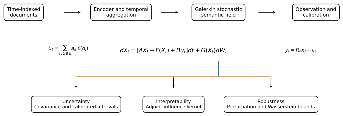
Figure 1 shows the passage from text to the three diagnostics. A corpus provides time-indexed documents. An encoder maps each document into a finite semantic representation. Aggregation over a prescribed time grid produces the forcing path. A Galerkin model propagates the latent state, while an observation equation links the state to ratings, labels, lexicon scores, or external responses. Filtering and likelihood estimation recover finite operators whose covariance and adjoint sensitivity approximate the infinite-dimensional quantities.

Let ${\{d_j,t_j,m_j\}}_{j=1}^{N_{\mathrm{doc}}}$ be a time-indexed corpus. The symbol $d_j$ denotes a document, and $m_j$ records its source together with any available annotation. A fixed encoder $\mathcal{E}$ maps $d_j$ to $z_j\in {\mathbb{R}}^p$. The encoder may be a transformer representation, a task-adapted language model, or an interpretable lexicon map. For a grid $0={\tau }_0<{\tau }_1<\cdots <{\tau }_L$, the forcing vector on the interval $[{\tau }_{\ell },{\tau }_{\ell +1})$ is

$$u_{\ell }=\sum _{j:t_j\in [{\tau }_{\ell },{\tau }_{\ell +1})}{a}_{j\ell }{z}_j.$$

(70)

The deterministic weights $a_{j\ell }$ may correct source imbalance or annotation reliability. Their normalisation is fixed before estimation in order to remove the scale ambiguity between $u_{\ell }$ and the lifting operator.

A semantic graph can be formed from encoded documents or from a set of semantic prototypes. Let $w_{ij}\ge 0$ be a symmetric similarity weight, and let $L_n$ be the corresponding graph Laplacian. If $e_k$ is a unit eigenvector with eigenvalue ${\lambda }_k$, then

$$e_k^{\mathsf{T}}{L}_n{e}_k={\displaystyle \frac{1}{2}}\sum _{i,j}{w}_{ij}{\left[e_k\left(i\right)-e_k\left(j\right)\right]}^2={\lambda }_k.$$

(71)

The eigenvalue is therefore the Dirichlet energy of the coordinate. Large values indicate rapid variation across semantically adjacent prototypes. Selecting the first n eigenvectors produces a low-frequency Galerkin space $H_n$. The truncation error for uncertainty and influence is controlled by Theorem 12.

Let $P_n:H\to H_n$ be the orthogonal projection. A consistent projected equation has the form

$$d{X}_t^{\left(n\right)}=\left[A_n{X}_t^{\left(n\right)}+F_n\left(X_t^{\left(n\right)}\right)+B_n{u}_t\right]dt+G_n\left(X_t^{\left(n\right)}\right)d{W}_t^{\left(n\right)}.$$

(72)

When $H_n\subset \mathrm{Dom}\left(A\right)$ and the basis is domain compatible, one may take $A_n=P_n{A|}_{H_n}$. A data-adapted basis requires a separately constructed generator whose semigroup converges consistently to S. The approximation theorem in Appendix A states a sufficient consistency condition.

In the linear additive regime, write $Q_n=G_n{G}_n^{\mathsf{T}}$. If the forcing is constant on an interval of length ${\Delta }_{\ell }$, the exact discrete transition is

$$x_{\ell +1}={\mathsf{F}}_{\ell }{x}_{\ell }+{\mathsf{D}}_{\ell }{u}_{\ell }+{\xi }_{\ell },{\xi }_{\ell }\sim \mathcal{N}(0,{\mathsf{\Omega }}_{\ell }),$$

(73)

where

$${\mathsf{F}}_{\ell }=e^{A_n{\Delta }_{\ell }},{\mathsf{D}}_{\ell }={\int }_0^{{\Delta }_{\ell }}{e}^{A_{n}s}{B}_{n}ds,{\mathsf{\Omega }}_{\ell }={\int }_0^{{\Delta }_{\ell }}{e}^{A_{n}s}{Q}_n{e}^{A_n^{\mathsf{T}}s}ds.$$

(74)

The use of the exact transition removes time-discretisation bias from the linear calibration problem. The observation equation is

$$y_{\ell }=R_n{x}_{\ell }+{\epsilon }_{\ell },{\epsilon }_{\ell }\sim \mathcal{N}(0,V_n).$$

(75)

The matrix $R_n$ links the latent state to the observed sentiment proxy. The covariance $V_n$ represents annotation or measurement variation, while $Q_n$ represents unresolved variation in the latent evolution.

For fixed parameters, the Kalman recursion supplies the likelihood and the filtered state covariance. With the standard notation for conditional means and covariances,

$${\widehat{x}}_{\ell +1|\ell }={\mathsf{F}}_{\ell }{\widehat{x}}_{\ell |\ell }+{\mathsf{D}}_{\ell }{u}_{\ell },P_{\ell +1|\ell }={\mathsf{F}}_{\ell }{P}_{\ell |\ell }{\mathsf{F}}_{\ell }^{\mathsf{T}}+{\mathsf{\Omega }}_{\ell }.$$

(76)

The innovation covariance and update are

$$\begin{array}{cc}\hfill S_{\ell +1}& =R_n{P}_{\ell +1|\ell }{R}_n^{\mathsf{T}}+V_n,\hfill \\ \hfill K_{\ell +1}& =P_{\ell +1|\ell }{R}_n^{\mathsf{T}}{S}_{\ell +1}^{-1},\hfill \\ \hfill {\widehat{x}}_{\ell +1|\ell +1}& ={\widehat{x}}_{\ell +1|\ell }+K_{\ell +1}\left[y_{\ell +1}-R_n{\widehat{x}}_{\ell +1|\ell }\right].\hfill \end{array}$$

(77)

Up to an additive constant, the Gaussian negative log-likelihood is

$$\mathcal{L}\left(\theta \right)={\displaystyle \frac{1}{2}}\sum _{\ell }\left[\log \det S_{\ell }+{\nu }_{\ell }^{\mathsf{T}}{S}_{\ell }^{-1}{\nu }_{\ell }\right],{\nu }_{\ell }=y_{\ell }-R_n{\widehat{x}}_{\ell |\ell -1}.$$

(78)

The parameter vector contains the finite representations of A, B, the process covariance, the observation map, and the observation covariance. A dissipative parameterisation is

$$A_n=-L_A{L}_A^{\mathsf{T}}-{\alpha }_0{I}_n+K_A,K_A^{\mathsf{T}}=-K_A,{\alpha }_0>0.$$

(79)

Its symmetric part is bounded above by $-{\alpha }_0{I}_n$. Cholesky factors enforce positive semidefiniteness of $Q_n$ and $V_n$. A dense Kalman likelihood costs $O\left(L{n}^3\right)$. Diagonal spectral dynamics reduce state propagation to $O\left(Ln\right)$, while low-rank observation maps permit intermediate complexity through matrix identities.

The operator $B_n$ is estimated from the conditional response to the aggregated text forcing. The generator $A_n$ is estimated under the dissipative constraint. A nonlinear drift can be parameterised by a differentiable map whose Jacobian has a controlled one-sided Lipschitz constant, thereby preserving a positive dissipativity margin. The process covariance is estimated from the residual state innovation after deterministic forcing has been accounted for. The observation covariance is identified from replicated annotation, known label reliability, or an explicit restriction separating measurement noise from process noise.

Proposition 4

(Identifiability of a linear projected model). Assume that $R_n=I_n$, that $V_n$ is known, and that the sampling interval is a fixed number $\Delta >0$. Suppose that the collection of conditional laws

$$\mathrm{Law}\left(y_{\ell +1}\mid x_{\ell }=x,u_{\ell }=u\right),x\in {\mathbb{R}}^n,u\in {\mathbb{R}}^p$$

is known. Assume that $\mathsf{F}=e^{A_n\Delta }$ has no eigenvalue on the closed negative real axis and that

$$\sigma (\Delta A_n)\subset \{z\in \mathbb{C}:|\mathrm{Im}z|<\pi \}.$$

Assume further that ${\int }_0^{\Delta }{e}^{A_{n}s}ds$ is invertible. Then, the conditional laws determine $A_n$, $B_n$, and ${\mathsf{\Omega }}_{\Delta }$. If the map

$${\mathcal{K}}_{\Delta }:Q⟼{\int }_0^{\Delta }{e}^{A_{n}s}Q{e}^{A_n^{\mathsf{T}}s}ds$$

is injective on the chosen covariance family, then the same laws determine $Q_n$. For finite-sample estimation of $\mathsf{F}$ and $\mathsf{D}$, the corresponding regressor matrix with rows $(x_{\ell }^{\mathsf{T}},u_{\ell }^{\mathsf{T}})$ must have full column rank.

Proof. 

The conditional law is Gaussian with mean

$$\mathsf{F}x+\mathsf{D}u$$

and covariance ${\mathsf{\Omega }}_{\Delta }+V_n$. Equality of the conditional means for every x and u identifies $\mathsf{F}$ and $\mathsf{D}$. The spectral assumptions place $\Delta A_n$ in the uniqueness strip of the principal matrix logarithm, so

$$A_n={\Delta }^{-1}\log \mathsf{F}.$$

The identity

$$\mathsf{D}=\left[{\int }_0^{\Delta }{e}^{A_{n}s}ds\right]B_n$$

and invertibility of the bracketed matrix identify $B_n$. The conditional covariance identifies ${\mathsf{\Omega }}_{\Delta }$ because $V_n$ is known. Injectivity of ${\mathcal{K}}_{\Delta }$ then identifies $Q_n$. The final rank condition is the standard uniqueness condition for estimating the coefficients of the conditional mean from finitely many observed pairs. □

The candidate corpora play distinct roles. Time-stamped social media data can construct $u_{\ell }$ and provide noisy labels. Review corpora provide longer evaluative units and document-level observations. Lexica provide externally anchored coordinates for $H_n$ or regularisation for $R_n$. These resources do not determine the operators automatically. They provide the observations, entering the likelihood, and the geometry, entering the basis construction.

The comparison with intelligent and structure-preserving solvers is made at the level of preserved objects. AI-enhanced symbolic derivation can propose closed-form identities and algebraic factorisations [31]. Physics-informed inverse methods can estimate projected coefficients from observations [28]. PDE denoising motivates a dissipative filtering stage [27]. Lie-group methods show how a numerical scheme can be designed around a geometric invariant [29]. Riemann–Hilbert analysis shows the value of exact spectral structure when integrability is present [30]. For the semantic-field equation, dissipativity is the discrete target. Hamiltonian energy preservation addresses a different geometry. A reliable high-order method should preserve contractivity up to a controlled defect, maintain positive semidefinite covariance, and converge jointly for the forward state and the adjoint influence equation. Neural SPDE solvers provide an alternative when the Galerkin dimension makes dense filtering impractical [25,26]. The covariance, duality, and truncation identities in Section 2 supply verification criteria for such solvers.

4. Synthetic Numerical Study

The numerical study uses a three-mode linear Galerkin model for which every transition and diagnostic is available in closed form. Its purpose is to test internal consistency, calibration feasibility, and the magnitude of the theoretical constants. The study does not represent a benchmark on natural language data.

Let $X_t\in {\mathbb{R}}^3$ solve

$$d{X}_t=\left[-\Lambda X_t+B{u}_t\right]dt+Q^{1/2}d{W}_t,Y_t=c^{\mathsf{T}}{X}_t+{\epsilon }_t,$$

(80)

where

$$\begin{array}{cc}\hfill \Lambda & =\mathrm{diag}(0.45,1.10,2.40),\hfill \\ \hfill B& =\left(\begin{array}{cc}0.90& 0.20\\ -0.25& 0.70\\ 0.15& -0.45\end{array}\right),\hfill \\ \hfill Q& =\mathrm{diag}(0.040,0.035,0.025),\hfill \\ \hfill c& ={(0.65,-0.55,0.35)}^{\mathsf{T}}.\hfill \end{array}$$

(81)

The observation noise has standard deviation $0.07$. The time step is $\Delta =0.15$, the number of transitions is 80, and the horizon is $T=12$. Each forcing coordinate combines a smooth oscillatory component with a localised pulse. Random amplitudes, phases, and pulse centres create trajectory-level heterogeneity. Initial states are Gaussian. The initial state, Brownian increments, observation errors, and random forcing parameters are mutually independent across trajectories. The random seed is 18082026.

The exact matrices in (74) are used for simulation. Twenty trajectories form the training sample, eighty independent trajectories form the conformal calibration sample, and four hundred independent trajectories form the test sample. The structured estimator uses a diagonal transition matrix with entries constrained to $(0,1)$, together with an unrestricted forcing matrix. A ridge regression estimates each modal transition and the two forcing coefficients. The readout is estimated by ridge regression on the latent states. The residual covariance estimates ${\mathsf{\Omega }}_{\Delta }$. The unrestricted vector autoregression with exogenous forcing and the persistence predictor provide finite-dimensional baselines.

The estimated damping rates are

$$0.470754,1.023585,2.370493.$$

The corresponding generating values are $0.45$, $1.10$, and $2.40$. The estimated readout is

$$\widehat{c}={(0.654022,-0.551861,0.338787)}^{\mathsf{T}}.$$

Table 1. One-step prediction performance on four hundred synthetic test trajectories.

Method	Readout RMSE	Readout MAE	Latent RMSE
Structured dissipative model	0.095182	0.076010	0.065492
Unrestricted VARX	0.095172	0.076004	0.065534
Persistence	0.104803	0.083764	0.075702

reports one-step performance on the test set.

For each test trajectory, the readout RMSE is computed over the eighty one-step forecasts. A paired bootstrap with five thousand resamples gives a mean structured-minus-VARX difference of $9.6960\times {10}^{-6}$, with percentile interval

$$[-1.3130\times {10}^{-5},3.3299\times {10}^{-5}].$$

The two-sided Wilcoxon signed-rank p-value is $0.4494$. The structured restriction therefore causes no detectable loss relative to the unrestricted VARX model in this experiment. The structured-minus-persistence difference is $-9.4908\times {10}^{-3}$, with interval

$$[-1.0052\times {10}^{-2},-8.9277\times {10}^{-3}],$$

and the two-sided Wilcoxon signed-rank p-value is $1.30\times {10}^{-66}$. These tests concern synthetic trajectories generated from (80). They do not support a claim about performance on a natural language benchmark.

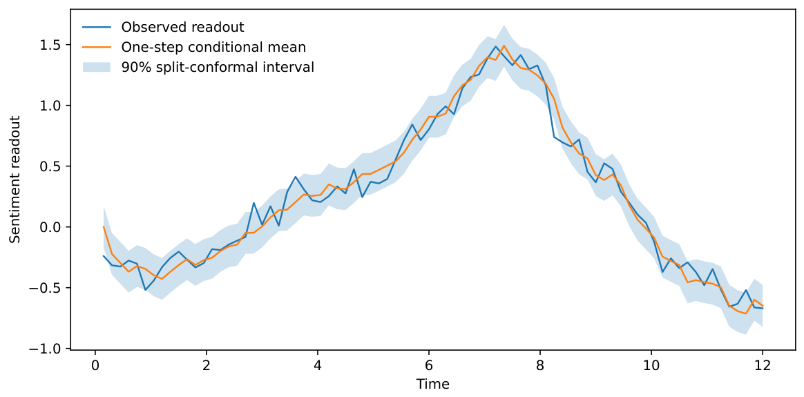
The estimated one-step predictive standard deviation is $0.094752$. Coverage is evaluated at the final one-step forecast of each independent test trajectory, so the calibration scores and the test scores are exchangeable conditional on the fitted predictor. A nominal Gaussian interval at level $0.90$ has empirical coverage $0.8800$, with Wilson interval $[0.8445,0.9083]$ and mean width $0.31170$. Split conformal calibration uses the eighty absolute standardised terminal residuals. The order statistic multiplier is $1.81583$. The resulting interval has empirical coverage $0.9175$, with Wilson interval $[0.8864,0.9407]$ and mean width $0.34411$. Proposition A4 in Appendix B gives the finite-sample marginal coverage statement. Figure 2 displays one representative trajectory and the interval obtained from the same conformal multiplier.

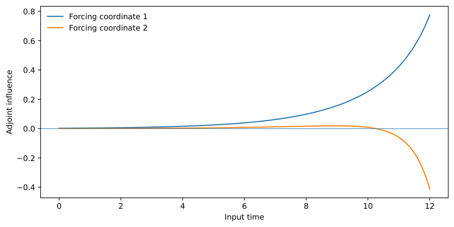
For the continuous model, the influence kernel of the terminal linear readout is

$${\mathcal{I}}_s=B^{\mathsf{T}}{e}^{-\Lambda (T-s)}c.$$

(82)

Numerical quadrature gives

$${\parallel \mathcal{I}\parallel }_{L^2(0,T;{\mathbb{R}}^2)}=0.752295.$$

For the input-energy radius $\rho =0.25$, Theorem 11 gives the exact worst-case terminal displacement

$${\rho \parallel \mathcal{I}\parallel }_{L^2}=0.1880738.$$

Substitution of the normalised extremal direction in (47) gives $0.1880738$ by numerical quadrature. The agreement verifies the dual identity to the displayed precision. Figure 3 shows how the two forcing coordinates contribute over time.

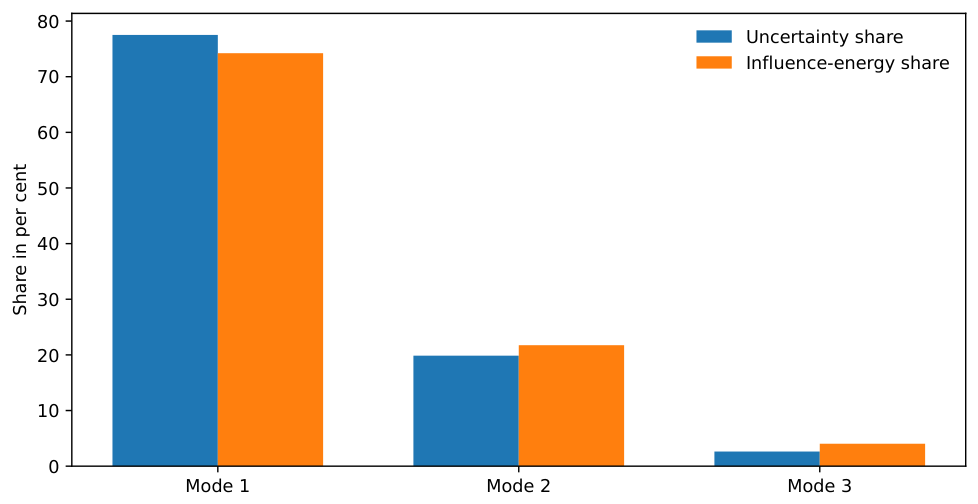
The exact variance contributions at horizon T are

$$0.0187774,0.0048125,0.0006380.$$

Their shares are $77.50$ percent, $19.86$ percent, and $2.63$ percent. For the identity lift diagnostic associated with Theorem 12, the corresponding influence-energy shares are $74.22$ percent, $21.74$ percent, and $4.04$ percent. The first two modes retain $97.37$ percent of the output variance and $95.96$ percent of the identity-lift influence energy. Figure 4 displays these quantities. The third coordinate represents local graph variation, so its small long-horizon contribution is the concrete counterpart of the high-frequency damping statement.

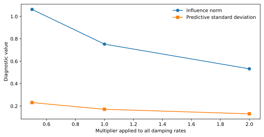
The analytic ablation in Theorem 2 is evaluated by multiplying every damping rate by $0.5$, 1, and 2.

Table 2. Dissipativity ablation at horizon $T=12$.

Damping Multiplier	Predictive Standard Deviation	Influence Norm	Semigroup Factor
0.5	0.230623	1.062181	1.487342
1.0	0.170669	0.752295	1.054082
2.0	0.130438	0.532025	0.745356

, see also Figure 5, shows the predictive standard deviation, the exact influence norm, and the semigroup factor

$${\kappa }_T\left({\lambda }_1\right)={\left[{\displaystyle \frac{1-e^{-2{\lambda }_{1}T}}{2{\lambda }_1}}\right]}^{1/2}.$$

Stronger damping lowers both uncertainty and influence. The values demonstrate that the dependence identified by the theorem is numerically informative in this regime.

A second ablation keeps $\mathrm{Tr}Q$ fixed and changes the noise geometry. The predictive standard deviation is $0.170669$ for diagonal noise, $0.151759$ for the stated positively correlated covariance, and $0.161189$ for isotropic noise with equal trace. The differences show that $\mathrm{Tr}Q$ alone cannot determine output uncertainty. Alignment with the readout and the damping spectrum is decisive.

The experiment gives an operational interpretation of the mathematical quantities. The covariance determines a predictive dispersion and a Gaussian reference interval. The influence kernel identifies the times and forcing directions that move the terminal mean. Its norm gives the exact energy-ball robustness radius in the linear regime. The truncation formula states how much uncertainty and influence are lost when modes are removed. The dissipativity margin controls the scale of all three diagnostics.

Limitations

The numerical evidence is synthetic and low dimensional. It verifies identities and tractability under controlled conditions, while leaving real-language validity unresolved. The training trajectories expose the latent state, whereas a corpus application would infer that state through the observation model. The global Lipschitz assumptions exclude discontinuous threshold responses and polynomial drifts without truncation or variational reformulation. The exact covariance study uses additive Gaussian noise. Heavy-tailed jumps, state-dependent non-Gaussian perturbations, and annotation processes with temporal dependence require different uncertainty tools. Split conformal coverage relies on exchangeability of the independent trajectory-level calibration and test scores. Distribution shift invalidates that guarantee unless a shift-aware conformal method is used. A large Galerkin basis can produce ill-conditioned likelihoods and weak identifiability when the forcing lacks persistent excitation. The synthetic baseline comparison does not establish superiority over transformer classifiers, large language models, conformal language model methods, or post hoc explanation algorithms. Such a claim requires a common real-data task, a fixed encoder, nested hyperparameter selection, and external benchmark evaluation.

5. Conclusions and Future Developments

A stochastic semantic field provides one evolution law for predictive uncertainty, forcing sensitivity, and perturbation stability. The covariance operator propagates latent variability to a terminal readout. The forcing-to-state map is Fréchet differentiable with a quadratic remainder, so the adjoint influence kernel represents a genuine bounded derivative. In the linear regime, the norm of that kernel equals the exact worst-case displacement over an input-energy ball. The spectral truncation formula then quantifies how finite semantic coordinates approximate both uncertainty and influence.

The projected model admits an exact continuous-to-discrete transition in the linear Gaussian case. This transition supports likelihood estimation and filtering without introducing a time-stepping error into calibration. The three-mode study confirms the covariance and duality identities, exhibits non-vacuous robustness constants, and shows how dissipativity changes predictive dispersion and influence. Split conformal calibration corrects the finite-sample coverage of the Gaussian interval in the synthetic experiment. These findings establish mathematical coherence and computational feasibility at the scale studied here.

A real-data investigation should begin with a fixed text encoder and a time-indexed corpus. The semantic graph, forcing aggregation, observation map, and projected dimension should be selected inside a nested validation design. Comparisons with transformer and large language model baselines should use a common predictive target and should report calibration, coverage, explanation stability, and perturbation response together with ordinary predictive loss. Distribution shift requires weighted or adaptive conformal methods. Partially observed latent states call for smoothing and data assimilation beyond the fully observed synthetic calibration.

The global Lipschitz setting can be extended through locally monotone or maximal monotone methods. Lévy noise can represent abrupt semantic shocks, while delay equations can model persistent influence from earlier information. Statistical consistency under a growing time horizon and a growing Galerkin dimension remains an important inverse problem. High-order numerical methods should preserve the dissipative structure and covariance positivity that enter the present estimates. Neural stochastic PDE solvers may reduce computational cost when their approximation errors are controlled in the state and adjoint equations.

Artificial-intelligence-enhanced mathematical derivation offers a further direction. A symbolic system guided by learned search can propose Lyapunov functionals, semigroup factorisations, covariance identities, and candidate adjoint representations. Every proposed identity must still be verified in the operator topology required by the theorem. Domain invariance for an unbounded generator, trace-class convergence, adaptedness of stochastic integrands, and passage from Yosida approximations to mild solutions remain mathematical obligations. The appropriate role of an automated derivation system is therefore the generation and checking of algebraic candidates within a proof workflow whose analytic hypotheses remain explicit.

The framework consequently defines a research programme in which infinite dimensional analysis determines the quantities that a finite estimator must preserve, numerical calibration makes those quantities observable, and external benchmarks determine whether the resulting representation is useful for a particular language domain.