Evaluation and Benchmarking of a Bounded Data-Driven Correction for Compartmental Pharmacokinetic Models

Abstract

Background/Objectives: This study applies the previously introduced structure-preserving hybrid framework for compartmental pharmacokinetic models and extends its clinical evaluation using published clinical datasets. The framework combines a mechanistic pharmacokinetic backbone with a bounded data-driven correction. The aim was to assess predictive performance in held-out subjects while keeping the main pharmacokinetic structure and avoiding a fully black-box model. Methods: This applied extension of the framework was tested in several numerical studies using published clinical pharmacokinetic datasets for polymyxin B, linezolid, and tacrolimus. For polymyxin B and linezolid, repeated subject-wise cross-validation with nested tuning was used to compare the mechanistic baseline with unconstrained and constrained hybrid corrections and a boosted-tree residual benchmark. The studies were designed to assess its behavior in a main application setting, across different drugs, under difficult fitting conditions, and under changes in correction strength and mechanistic parameters. Computational time was also assessed. Results: The results showed that the constrained correction remained close to the mechanistic baseline in the held-out analyses of polymyxin B and linezolid, but it did not significantly improve subject-level prediction. The unconstrained correction showed greater deterioration, while the boosted-tree benchmark gave mixed results and no significant subject-level improvement. The additional analyses showed that tighter correction bounds were generally selected and that the constrained hybrid still responds to changes in the mechanistic parameters in a sensible manner. Conclusions: Overall, the results suggest that the bounded data-driven correction can control the poorer performance seen with an unrestricted correction while keeping prediction close to the mechanistic baseline. It therefore provides a cautious way to combine mechanistic pharmacokinetic modeling with data-driven correction while preserving interpretability. Further external validation is still needed.

1. Introduction

Pharmacokinetic (PK) modeling remains one of the main tools used to describe drug absorption, distribution, and elimination, and it continues to play an important role in dose selection, therapeutic drug monitoring, and individualized treatment planning [1,2,3,4]. Classical compartmental and population PK models are still widely used because they are interpretable, physiologically meaningful, and acceptable in clinical and regulatory settings [1,2,5]. However, these models depend on assumptions that may not explain all the variability seen in heterogeneous patient groups or in datasets with limited sampling [2,3,4]. Therefore, there is still a need for models that keep the mechanistic basis of PK modeling but can also account for patterns that are not explained by the original model. This is important in model-informed precision dosing, where the model should support dose adjustment while remaining understandable in clinical practice [2,3,4].

Machine-learning and neural differential equation methods have also been used in PK modeling because they can learn patterns that may be missed by standard models [6,7,8,9]. However, fully data-driven models may be difficult to interpret, may perform poorly outside the data used for training, and may not preserve basic PK properties such as positivity and compartmental consistency [6,7,8]. Hybrid models try to address this by combining mechanistic equations with a learned correction [7,8,9]. Existing hybrid approaches differ in how the learned component is incorporated and controlled. In particular, not all formulations explicitly limit the correction relative to the mechanistic dynamics or examine whether a constrained formulation remains useful under held-out evaluation in different clinical datasets. The present work focuses on this setting by evaluating a bounded correction across published pharmacokinetic datasets with different drugs, dosing structures, and covariate profiles.

This issue is important for drugs with narrow therapeutic ranges or large differences between patients. Tacrolimus, linezolid, and polymyxin B were selected because they represent different clinical settings, including therapeutic drug monitoring, pediatric anti-infective treatment, and treatment of critically ill patients [5,10,11,12,13,14]. The three datasets also differ in their dosing, sampling, and available covariates. They were therefore used to examine whether the framework could be applied across different clinical datasets rather than only in one setting. The central research question of the present study is therefore whether a structure-preserving hybrid PK model can improve or preserve predictive performance under held-out evaluation without losing the mechanistic properties that make PK models useful in practice.

In our earlier work [15], we introduced the general structure-preserving formulation for compartmental PK models, where the learned correction was bounded so that the main mechanistic behavior of the system was not lost. That study established the general formulation and examined its main theoretical and numerical properties. The present study extends this work by examining its performance across published clinical pharmacokinetic datasets, including held-out evaluation in the polymyxin B and linezolid datasets. We therefore applied it to three published clinical datasets involving different drugs, dosing routes, compartmental structures, sampling patterns, and covariate information. We also considered a more difficult case in which the mechanistic baseline was weak. In addition, the present work includes repeated subject-wise cross-validation with nested tuning for polymyxin B and linezolid, comparison with a boosted-tree residual benchmark, further analysis of correction strength, mechanistic parameter sensitivity, computational time, and subject-level performance. Together, these clinical applications and additional analyses form the main contribution of the present study. Unlike many general PK/ADMET or purely data-driven machine-learning tools, the method used in the present study starts from a fitted mechanistic PK model and applies a bounded correction to its concentration predictions rather than predicting drug properties directly from chemical descriptors.

2. Materials and Methods

2.1. Structure-Preserving Hybrid Pharmacokinetic Framework

We consider a compartmental pharmacokinetic model written in terms of drug amounts. Let $A_i(t)$ denote the amount of drug in compartment $i$ at time $t$, for $i=1,\dots ,n$, and let $C_i(t)=A_i(t)/V_i$ denote the corresponding concentration, where $V_i$ is the volume of that compartment. The mechanistic model is written as

$${\displaystyle \frac{d{A}_i}{dt}}=F_i\left(A,\theta ,z,u,t\right), i=1,\dots ,n,$$

(1)

where $A=(A_1,\dots ,A_n{)}^{\mathrm{\top }}$ is the state vector, $\theta$ is the parameter vector, $z$ denotes observed covariates, and $u$ represents known inputs such as dose administration. The functions $F_i$ describe the usual PK processes, including absorption, transfer between compartments, distribution, and elimination. This formulation is sufficiently general for the one- and two-compartment settings considered in the present study.

In the general ODE-based formulation introduced in [15], the hybrid model is obtained by adding a learned correction term to the mechanistic system. Thus, we write

$${\displaystyle \frac{d{A}_i}{dt}}=F_i\left(A,\theta ,z,u,t\right)+G_i\left(A,z,u,t;\varphi \right), i=1,\dots ,n,$$

(2)

where $G_i$ is a data-driven correction with parameter vector $\varphi$. The mechanistic component remains central in the formulation. This formulation provides the general basis for the bounded-correction approach used in the present study.

Within this formulation, the correction is controlled by

$$\left|G_i\left(A,z,u,t;\varphi \right)\right|\le {\alpha }_i\hspace{0.17em}{\mathsf{\Psi }}_i\left(A,\theta ,z,u,t\right),$$

(3)

where ${\alpha }_i>0$ is a control parameter and ${\mathsf{\Psi }}_i$ is a suitable reference scale derived from the mechanistic model. This condition limits the correction relative to the main PK dynamics. When an internal transfer term is modified, the correction is constructed to preserve compartmental balance, and it is restricted accordingly when nonnegative state variables are required. These conditions apply to the general ODE-level formulation, while the output-level implementation used in the present numerical studies is described below.

For the numerical studies, the bounded correction was applied to the mechanistic concentration prediction at the output level and expressed on the logarithmic concentration scale. Let $z_{\varphi }(x)$ denote the fitted correction function based on the standardized hybrid features. The constrained correction was defined as ${\delta }_{\mathrm{c}\mathrm{o}\mathrm{n}}(x)=\alpha \mathrm{t}\mathrm{a}\mathrm{n}\mathrm{h}(z_{\varphi }(x))$, and the final prediction was calculated as ${\widehat{C}}_{\mathrm{h}\mathrm{y}\mathrm{b}}=\mathrm{e}\mathrm{x}\mathrm{p}\{\mathrm{l}\mathrm{o}\mathrm{g}({\widehat{C}}_{\mathrm{m}\mathrm{e}\mathrm{c}\mathrm{h}}+\epsilon )+{\delta }_{\mathrm{c}\mathrm{o}\mathrm{n}}(x)\}$, where $\epsilon >0$ is a small constant used to avoid taking the logarithm of zero. This formulation ensures that $\mid {\delta }_{\mathrm{c}\mathrm{o}\mathrm{n}}(x)\mid \le \alpha$. The correction function included linear terms with or without radial basis functions and was estimated by ridge-regularized least squares. The hyperbolic tangent was used because it provides a smooth and differentiable bound rather than abrupt clipping. For the held-out polymyxin B and linezolid analyses, the value of $\alpha$ was selected during nested inner validation. For illustration, when $\alpha =0.35$, the correction is limited approximately to a multiplicative range of $\mathrm{e}\mathrm{x}\mathrm{p}(-0.35)$ to $\mathrm{e}\mathrm{x}\mathrm{p}(0.35)$, corresponding to about 0.70 to 1.42 times the mechanistic prediction. Since $\mid {\delta }_{\mathrm{c}\mathrm{o}\mathrm{n}}(x)\mid \le \alpha$, the corrected prediction satisfies $e^{-\alpha }({\widehat{C}}_{\mathrm{m}\mathrm{e}\mathrm{c}\mathrm{h}}+\epsilon )\le {\widehat{C}}_{\mathrm{h}\mathrm{y}\mathrm{b}}\le e^{\alpha }({\widehat{C}}_{\mathrm{m}\mathrm{e}\mathrm{c}\mathrm{h}}+\epsilon )$. Therefore, a positive mechanistic prediction remains positive after correction, and the learned component cannot move the prediction beyond the prescribed multiplicative range. The smoothness of the hyperbolic tangent also avoids discontinuities in the corrected prediction.

2.2. Population Pharmacokinetic Setting and Estimation

The present work is carried out in a population-oriented PK setting, in which parameters may vary across individuals through observed covariates and, in the general formulation, random effects. At the structural level, this is written as

$$\theta =\theta \left(z,\eta \right),$$

(4)

where $z$ contains observed covariates and $\eta$ denotes interindividual variability. In this way, the mechanistic model retains the main PK interpretation, while the learned correction is used only for residual systematic effects that remain after the structural model and covariate relations have been introduced. Parameters such as clearance, volume, and absorption rate therefore continue to play their usual role in the formulation. In the present numerical studies, subject-specific parameters were represented using the available covariate relations, and a full nonlinear mixed-effects estimation of random effects was not performed.

Let $Y_{ij}$ denote the measured concentration for subject $j$ at time $t_{ij}$. The observation model is written as

$$Y_{ij}=\mathcal{H}\left(A_j\left(t_{ij}\right)\right)+{\epsilon }_{ij},$$

(5)

where $\mathcal{H}$ maps the compartmental state to the observed quantity and ${\epsilon }_{ij}$ denotes residual error. Parameter estimation is based on an objective function that combines data fit with control of the correction term. For the output-level implementation used in the numerical studies, let $\delta$ denote the correction applied to the mechanistic concentration prediction. A general form of the objective function is

$$\mathcal{L}={\mathcal{L}}_{\mathrm{d}\mathrm{a}\mathrm{t}\mathrm{a}}+\lambda \hspace{0.17em}\mathcal{R}\left(\delta \right),$$

(6)

where ${\mathcal{L}}_{\mathrm{d}\mathrm{a}\mathrm{t}\mathrm{a}}$ measures the discrepancy between observed and predicted concentrations, $\mathcal{R}(\delta )$ penalizes excessive correction size or behavior inconsistent with the intended structure, and $\lambda >0$ is a regularization parameter. The exact residual model and regularization term may differ across drugs, but the same general framework is used throughout the study.

In the numerical studies, the mechanistic parameters were estimated using nonlinear least squares. For the held-out polymyxin B and linezolid analyses, the mechanistic parameters were re-estimated using only the training subjects within each fold. The correction model combined standardized linear features with or without radial basis functions and was fitted using ridge-regularized least squares. The correction form, regularization level, and correction-strength parameter were selected using nested inner validation, as described below. The correction parameters were obtained by solving the regularized linear system directly. Convergence of the mechanistic fitting was assessed using the predefined function and step tolerances.

2.3. Mathematical Properties of the Hybrid Model

The analysis below concerns the general ODE-based hybrid formulation in (2), together with the control condition in (3), the population parameter relation in (4), and the observation structure in (5) and (6). We assume that the functions appearing in (1) and (2) are continuous in time, continuously differentiable with respect to the state and parameter variables, and continuous in the remaining variables on the region of interest.

Proposition 1.  

Assume that the vector field defined by the right-hand side of (2) is locally Lipschitz in the state variable, uniformly with respect to the parameters and patient descriptors on bounded sets. Then, for every initial condition, the hybrid system admits a unique local solution. Moreover, the solution depends continuously on the initial data, the mechanistic parameters, the correction parameters, and the patient descriptors appearing in (4).

Small changes in the patient covariates or parameter values do not lead to abrupt changes in the PK trajectory, at least on finite time intervals where the solution exists. This is important in the present setting because the same framework is used across different patients and different clinical datasets. A proof is given in Appendix A. The result is a standard consequence of local Lipschitz continuity, but here it is used in a population-oriented PK setting where the model depends explicitly on patient descriptors [16].

Proposition 2.  

Let $S_{\theta }(t)$ denote the sensitivity matrix of the hybrid model with respect to the mechanistic parameters, and let $S_{\theta }^{\hspace{0.17em}0}(t)$ denote the corresponding sensitivity matrix for the mechanistic model in (1). Assume that the derivatives of the correction term with respect to the state and, if present, with respect to the mechanistic parameters are bounded on the region of interest, and that their combined size is at most $\epsilon >0$. Then, on every finite time interval on which both solutions remain in that region, there exists a constant $C_T>0$, depending on the interval and on bounds of the mechanistic system but independent of $\epsilon$, such that

$$‖S_{\theta }\left(t\right)-S_{\theta }^{\hspace{0.17em}0}(t)‖\le C_T\epsilon$$

If the correction remains sufficiently controlled, then the way the hybrid model responds to changes in the mechanistic parameters stays close to the response of the base PK model. This matters because quantities such as clearance, volume, and absorption rate should still retain their main PK meaning after the correction is introduced. This behavior was discussed qualitatively in [15], while Proposition 2 gives an explicit finite-time bound under the stated derivative condition. This result follows from the variational equations associated with (1) and (2), together with the stated derivative bound on the correction term and a Grönwall-type estimate. The proof is included in Appendix A.

Proposition 3.  

Suppose that, for the mechanistic model observed through (5), the parameter-to-observation map is locally distinguishable at a reference parameter value, in the sense that the corresponding sensitivity matrix has full column rank on the observation window of interest. Assume further that the observation map $H$ is continuously differentiable, and that the correction term is continuously differentiable and satisfies the smallness condition used in Proposition 2. Then there exists ${\epsilon }_0>0$  such that, whenever that smallness condition holds with threshold ${\epsilon }_0$, the hybrid model preserves local distinguishability of the mechanistic parameters on the same observation window.

If the mechanistic parameters can be locally separated in the base model, then a sufficiently controlled correction does not destroy that property. In practical terms, the main PK parameters remain locally distinguishable as long as the learned term does not compete too strongly with them. This point was discussed qualitatively in [15], while Proposition 3 gives a local rank-based result under the stated smallness condition. This proposition does not claim full structural identifiability of the joint parameter set. It is a local result for the mechanistic parameters in the presence of a constrained correction. The argument relies on continuity of matrix rank under sufficiently small perturbations and is given in Appendix A.

In the general model, if a correction is added to a transfer term, it is added with opposite signs in the two compartments. In this way, the correction only changes the movement of the drug between compartments and does not add or remove drug from the system. Equation (3) also keeps the size of this correction limited relative to the mechanistic model. These statements refer to the general ODE-level formulation.

For the output-level implementation used in the numerical analyses, positivity and bounded correction size follow directly from the form of the corrected prediction. Propositions 1–3 concern the general ODE-based formulation and provide the analytical basis for its population-oriented extension.

2.4. Datasets and Numerical Implementation

We tested the framework using three published clinical pharmacokinetic datasets. The datasets were selected because they contained concentration-time data together with dosing information and relevant patient covariates, and because they represented different drugs, dosing routes, and model structures. Each dataset was analyzed separately and the datasets were not combined into a single training dataset. Repeated subject-wise validation was used for polymyxin B and linezolid, whereas tacrolimus was evaluated as an exploratory in-sample robustness study. No independent external validation dataset was used. The numerical studies are organized by purpose. We begin with a primary clinical application on polymyxin B, followed by cross-drug evaluation and a robustness study in a more difficult clinical setting. Only records with a valid observed concentration were included in the analysis. Missing concentration values were excluded and were not imputed. We first consider the polymyxin B dataset from Hanafin et al. 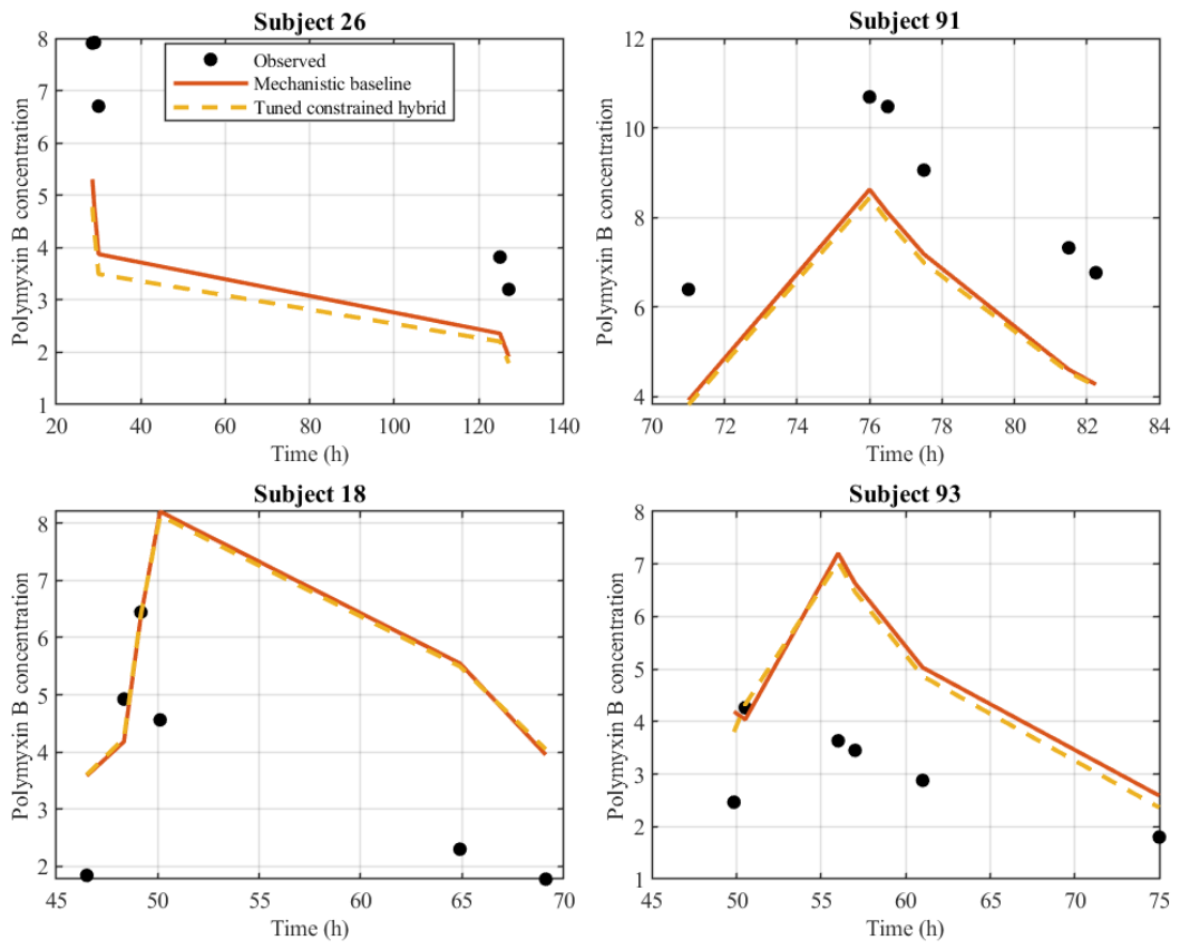[13]. This dataset was chosen as the first main application because it gives a clinically important setting with explicit intravenous infusion records and a mechanistic structure that is suitable for a full comparison. In our implementation, the dataset contained 40 subjects, 268 dosing events, and 230 concentration observations. The data was provided in event format, with explicit entries for dose amount, infusion rate, and infusion duration. Therefore, in this case we did not need to reconstruct oral absorption, lag time, or repeated dosing from simplified summaries. The infusion events were taken directly from the file and used as they were. For the mechanistic baseline, we used a two-compartment intravenous infusion model with elimination from the central compartment. The numerical model was

$$\begin{gathered} {\displaystyle \frac{d{A}_1}{dt}}=R_{\mathrm{i}\mathrm{n}}(t)-\left({\displaystyle \frac{C{L}_i}{V_{C,i}}}+{\displaystyle \frac{Q_i}{V_{C,i}}}\right)A_1+{\displaystyle \frac{Q_i}{V_{P,i}}}{A}_2, \\ {\displaystyle \frac{d{A}_2}{dt}}={\displaystyle \frac{Q_i}{V_{C,i}}}{A}_1-{\displaystyle \frac{Q_i}{V_{P,i}}}{A}_2, \end{gathered}$$

where $A_1$ and $A_2$ are the drug amounts in the central and peripheral compartments, respectively, and $R_{\mathrm{i}\mathrm{n}}(t)$ is the infusion input rate. The subject-specific parameters were scaled by body weight, and clearance also included a creatinine clearance effect. In the final mechanistic baseline, the predicted concentration was taken as

$${\widehat{C}}_{\mathrm{m}\mathrm{e}\mathrm{c}\mathrm{h}}\left(t\right)={\displaystyle \frac{A_1(t)}{V_{C,i}}}+C_0.$$

Among the mechanistic runs we tested, this offset version gave the best baseline fit and was therefore retained as the mechanistic model structure in this application.

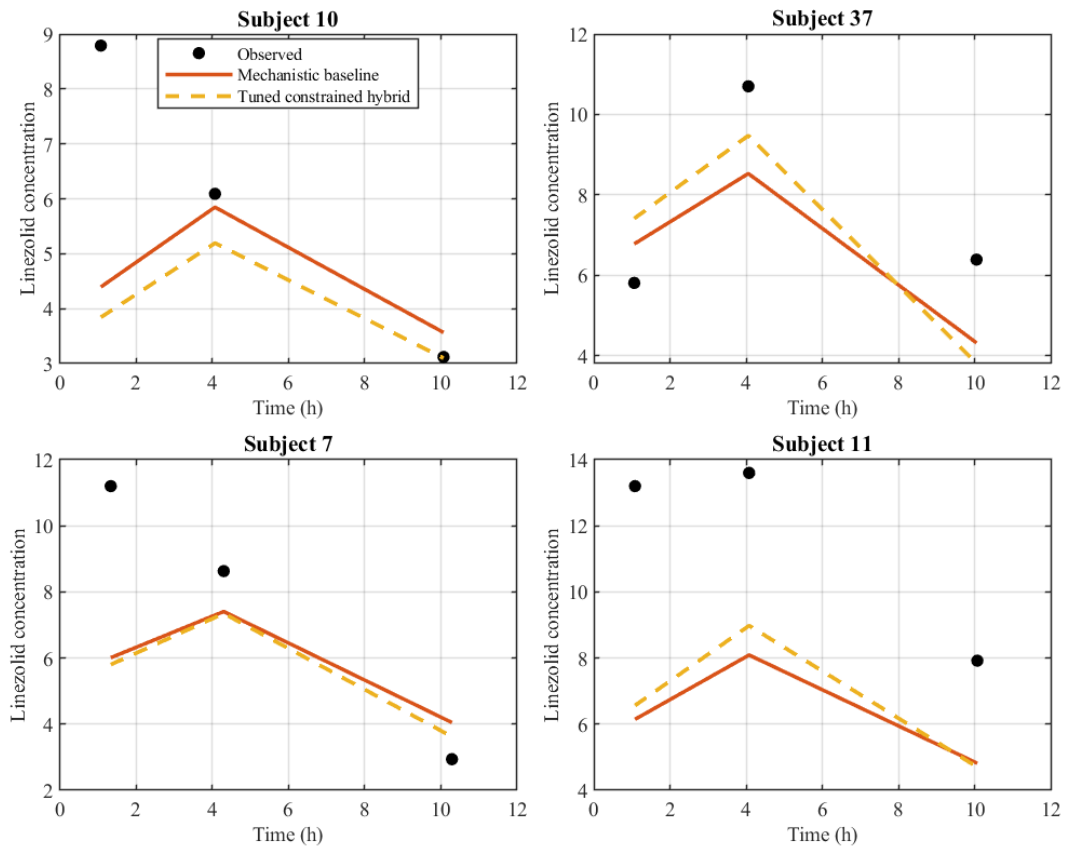
We next considered linezolid as a cross-drug evaluation study using the published dataset from [12], where the purpose was to assess the held-out predictive performance of the framework in a different pharmacokinetic setting. In this case, the data corresponded to oral or nasogastric administration, so the mechanistic baseline was simpler than in the polymyxin B study. After data cleaning and dose expansion, the dataset used in our implementation contained 48 subjects, 305 dose events, and 196 concentration observations.

For the mechanistic baseline, we used a one-compartment model with first-order absorption and first-order elimination. The numerical model was

$${\displaystyle \frac{d{A}_g}{dt}}=-K_a{A}_g, {\displaystyle \frac{d{A}_c}{dt}}=K_a{A}_g-{\displaystyle \frac{C{L}_i}{V_i}}{A}_c,$$

where $A_g$ and $A_c$ denote the amounts in the absorption and central compartments, respectively. The predicted concentration was taken as

$${\widehat{C}}_{mech}(t)={\displaystyle \frac{A_c(t)}{V_i}}.$$

The subject-specific parameters were scaled by body weight, and the mechanistic parameters were re-estimated using only the training subjects within each outer fold.

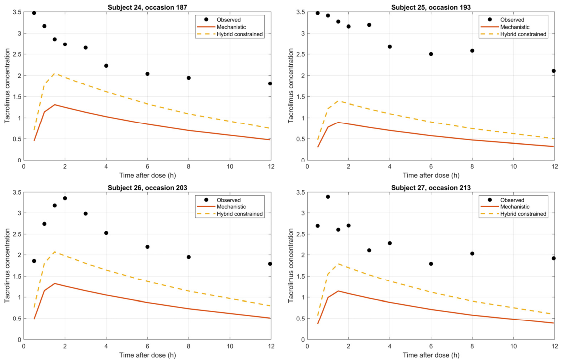
We next considered the published tacrolimus dataset of Quintairos et al. as an exploratory robustness study [17]. The role of this experiment was different from the first two studies. Here, the goal was to test whether the framework could reduce in-sample prediction error when the baseline model is weak and the data are more difficult. This is a harder setting because tacrolimus is well known for large variability, and in our implementation the data were naturally handled at the occasion level using the observed time-after-dose values. After preprocessing, the dataset used in this study contained 471 occasions and 1102 concentration observations. For the mechanistic baseline, we used an oral two-compartment model with first-order absorption, lag time, and elimination from the central compartment. The numerical model was

$$\begin{gathered} {\displaystyle \frac{d{A}_g}{dt}}=-K_a{A}_g, \\ {\displaystyle \frac{d{A}_c}{dt}}=K_a{A}_g-\left({\displaystyle \frac{C{L}_i}{V_{C,i}}}+{\displaystyle \frac{Q_i}{V_{C,i}}}\right)A_c+{\displaystyle \frac{Q_i}{V_{P,i}}}{A}_p, \\ {\displaystyle \frac{d{A}_p}{dt}}={\displaystyle \frac{Q_i}{V_{C,i}}}{A}_c-{\displaystyle \frac{Q_i}{V_{P,i}}}{A}_p, \end{gathered}$$

where $A_g,$ $A_c,$ and $A_p$ denote the amounts in the absorption, central, and peripheral compartments, respectively. The predicted concentration was taken as

$${\widehat{C}}_{\mathrm{m}\mathrm{e}\mathrm{c}\mathrm{h}}\left(t\right)={\displaystyle \frac{A_c\left(t\right)}{V_{C,i}}}.$$

Across all three numerical studies, the correction was applied to the mechanistic concentration prediction at each observation time. The hybrid component did not directly estimate or modify pharmacokinetic parameters such as clearance, volume of distribution, intercompartmental clearance, absorption rate, or lag time. These parameters remained part of the fitted mechanistic baseline. The main predicted endpoint was drug concentration, and model performance was assessed by comparing the predicted and observed concentrations. For polymyxin B and linezolid, predictive performance was assessed in held-out subjects. For tacrolimus, the reported comparison was exploratory and in-sample.

2.5. Model Comparison and Sensitivity Analyses

Whenever relevant, we compare the mechanistic baseline with unconstrained and constrained hybrid models and, for polymyxin B and linezolid, with a boosted-tree residual benchmark to examine whether the correction improves or preserves held-out predictive performance while remaining controlled relative to the mechanistic baseline. Model performance was assessed using the root mean square error (RMSE), mean absolute error (MAE), median absolute error (MedAE), correlation coefficient, and logarithmic root mean square error (LogRMSE).

For the polymyxin B and linezolid analyses, we used repeated five-fold subject-wise cross-validation with five repeats. All records from the same subject were kept within the same fold. In each repeat, the mechanistic model and the correction models were fitted using the outer training subjects and evaluated using only the held-out subjects. Within each outer training set, four-fold subject-wise inner validation was used for model selection. The mechanistic parameters were re-estimated using only the inner training subjects. Any covariate imputation, feature standardization, and radial basis function center selection were also based only on the corresponding training data.

The candidate correction models included a linear-only form and radial basis function forms with 4, 8, or 12 centers. Ridge regularization values of 0.01, 0.1, 1, and 10 were tested. For the constrained correction, values $\alpha \in \left\{\mathrm{0.10,0.15,0.25,0.35}\right\}$ were considered. This gave 16 unconstrained and 64 constrained candidates. The unconstrained and constrained models were selected separately according to the mean subject-level MAE in the inner validation folds. After selection, the correction was fitted using the complete outer training set and evaluated using the held-out outer subjects.

The boosted-tree residual benchmark was fitted to the same log-scale residual target and standardized features used by the correction models. It used least-squares gradient boosting with 150 regression stumps, a learning rate of 0.05, and a minimum leaf size of 5 observations. These settings were fixed before the outer held-out evaluation.

The effect of the correction-strength parameter was examined through its selection during nested inner validation. The frequency with which each value of $\alpha$ was selected across the 25 outer folds was recorded separately for polymyxin B and linezolid. No single value of $\alpha$ was fixed for the held-out analyses.

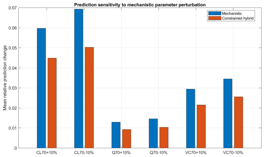
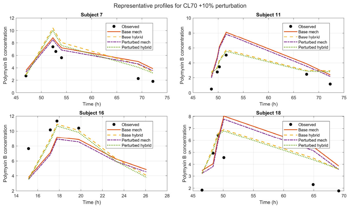
We finally checked whether the constrained hybrid model still responds to changes in the main mechanistic parameters in a sensible way. This test was done on the polymyxin B dataset, since this was the main application and gave the clearest baseline model. The aim here was to see whether the hybrid correction keeps the main effect of the mechanistic parameters or hides it completely. We considered three parameters from the mechanistic model, namely $C{L}_{70}$, $V_{C,70}$, and $Q_{70}$, and perturbed each of them by $\pm 10\mathrm{\%}$ while keeping the remaining parts of the model fixed. This separate analysis used $\alpha =0.35$ and was treated as a local in-sample interpretability analysis rather than a held-out predictive comparison.

Computational time was assessed for the polymyxin B application using one unrecorded warm-up run followed by three measured runs on the same computer. The mechanistic prediction, feature construction, correction fitting, bounded transformation, and final hybrid prediction were timed separately. Data loading, file writing, and figure generation were excluded. The timing results are reported as mean $\pm$standard deviation. This timing comparison concerned one mechanistic fit and one correction fit and did not include the repeated cross-validation or nested model-selection procedure.

For each outer repeat, the held-out predictions from the five outer folds were combined before the overall performance metrics were calculated. These metrics were then summarized across the five repeats using the mean and standard deviation. To examine performance across subjects, the MAE was calculated separately for each subject using its held-out predictions and then averaged across the five repeats. Paired subject-level differences were defined as the mechanistic MAE minus the comparator MAE, so that a positive value indicated improvement over the mechanistic model. The paired values were compared using a two-sided Wilcoxon signed-rank test, and the rank-biserial effect size was calculated. Ninety-five percent confidence intervals for the mean and median paired differences were estimated using 10,000 subject-level bootstrap samples. The constrained-versus-mechanistic comparison was the main comparison, while the unconstrained and boosted-tree comparisons were additional comparisons. A $p$-value below 0.05 was considered statistically significant.

3. Results

3.1. Primary Clinical Application: Polymyxin B

For the repeated held-out polymyxin B analysis, the mechanistic model was re-estimated within each training fold and compared with two tuned hybrid corrections and a boosted-tree residual benchmark. The first was an unconstrained hybrid model, where a learned correction was added on the logarithmic scale to the mechanistic prediction. The second was a constrained hybrid model, where a correction of the same form was bounded smoothly so that it remained controlled relative to the mechanistic baseline. Thus, four models were compared in this study, the mechanistic baseline, the tuned unconstrained hybrid, the tuned constrained hybrid, and the boosted-tree residual benchmark.

The main results are summarized in

Table 1. Held-out predictive performance in the primary polymyxin B application using repeated subject-wise cross-validation and nested model selection. Values are the mean (SD) across five repeats.

Model	RMSE	MAE	MedAE	Correlation	LogRMSE
Mechanistic	2.432 (0.040)	1.879 (0.036)	1.536 (0.028)	0.712 (0.011)	0.482 (0.013)
Unconstrained hybrid	3.032 (0.423)	2.181 (0.225)	1.661 (0.170)	0.600 (0.066)	0.563 (0.072)
Constrained hybrid	2.516 (0.060)	1.943 (0.070)	1.599 (0.107)	0.695 (0.017)	0.499 (0.015)
Boosted-tree benchmark	2.707 (0.214)	2.074 (0.139)	1.684 (0.108)	0.679 (0.019)	0.517 (0.027)

. The mechanistic baseline gave the best overall held-out predictive metrics. The mean MAE across the five repeats was 1.8788 for the mechanistic model, 2.1805 for the tuned unconstrained hybrid, 1.9427 for the tuned constrained hybrid, and 2.0742 for the boosted-tree benchmark. Among the data-driven models, the constrained hybrid remained closest to the mechanistic baseline and showed less deterioration than the unconstrained correction. This is the main idea of the bounded-correction approach used in the present study. The goal is not only to reduce the prediction error, but also to keep the learned correction under control and preserve the role of the mechanistic model. The held-out results therefore support the value of the constraint in controlling residual learning, although they do not show an overall predictive improvement over the mechanistic model. At the subject level, the constrained hybrid had a lower mean absolute error in 16 of the 40 subjects. The median subject-level mean absolute error was 1.7895 for the mechanistic model and 1.9146 for the constrained hybrid. The difference did not reach statistical significance in the two-sided Wilcoxon signed-rank test ($p=0.106$). The complete patient-level paired results, including the bootstrap confidence intervals and rank-biserial effect sizes, are reported in

Table A1. Patient-level paired results for the polymyxin b held-out analysis.

Comparator	Median MAE Difference (95% CI)	Mean MAE Difference (95% CI)	Wilcoxon p	Rank-Biserial Effect	Improved, n/N (%)
Unconstrained hybrid	−0.120 (−0.263 to −0.020)	−0.324 (−0.651 to −0.069)	0.007	−0.483	13/40 (32.5%)
Constrained hybrid	−0.080 (−0.203 to 0.040)	−0.066 (−0.160 to 0.031)	0.106	−0.295	16/40 (40.0%)
Boosted-tree benchmark	−0.084 (−0.206 to 0.089)	−0.209 (−0.418 to −0.030)	0.146	−0.266	18/40 (45.0%)

. In comparison, the unconstrained hybrid was significantly worse than the mechanistic baseline at the subject level ($p=0.007$).

Representative held-out subject profiles are shown in Figure 1. The mechanistic model captures the general trend, while the constrained hybrid generally remains close to the mechanistic prediction. The profiles show that the correction can reduce part of the mismatch in some subjects but does not do so consistently across all subjects. Together with the results in Table 1, this indicates that the constrained correction limits the larger changes seen with unrestricted residual learning without demonstrating overall superiority to the mechanistic baseline.

3.2. Cross-Drug Evaluation: Linezolid

For the repeated held-out linezolid analysis, the mechanistic model was re-estimated within each training fold and compared with the tuned unconstrained and constrained hybrid models and the boosted-tree residual benchmark. The main results are summarized in

Table 2. Held-out predictive performance in the linezolid evaluation using repeated subject-wise cross-validation and nested model selection. Values are mean (SD) across five repeats.

Model	RMSE	MAE	MedAE	Correlation	LogRMSE
Mechanistic	3.876 (0.027)	2.767 (0.019)	1.785 (0.052)	0.647 (0.008)	0.569 (0.003)
Unconstrained hybrid	4.272 (0.581)	2.937 (0.234)	1.839 (0.040)	0.588 (0.039)	0.587 (0.018)
Constrained hybrid	3.937 (0.055)	2.782 (0.054)	1.908 (0.073)	0.615 (0.011)	0.582 (0.008)
Boosted-tree benchmark	3.755 (0.093)	2.683 (0.051)	1.847 (0.071)	0.673 (0.019)	0.550 (0.008)

. The tuned constrained hybrid remained close to the mechanistic baseline, while the unconstrained correction showed poorer overall held-out performance.

The mean held-out MAE across the five repeats was 2.7667 for the mechanistic model, 2.9371 for the tuned unconstrained hybrid, 2.7824 for the tuned constrained hybrid, and 2.6832 for the boosted-tree benchmark. The constrained hybrid therefore remained close to the mechanistic baseline and performed better overall than the unconstrained correction, but it did not provide a clear improvement over the mechanistic model.

At the subject level, the constrained hybrid had a lower MAE in 26 of the 48 subjects. The median subject-level MAE was 2.1177 for the mechanistic model and 2.2410 for the constrained hybrid. The paired difference was not statistically significant in the two-sided Wilcoxon signed-rank test (p = 0.867). The boosted-tree benchmark gave the lowest overall mean MAE, but its subject-level difference from the mechanistic model was also not statistically significant (p = 0.467). The complete patient-level paired results are reported in

Table A2. Patient-level paired results for the linezolid held-out analysis.

Comparator	Median MAE Difference (95% CI)	Mean MAE Difference (95% CI)	Wilcoxon p	Rank-Biserial Effect	Improved, n/N (%)
Unconstrained hybrid	−0.002 (−0.097 to 0.085)	−0.102 (−0.228 to 0.009)	0.401	−0.141	24/48 (50.0%)
Constrained hybrid	0.018 (−0.072 to 0.070)	−0.004 (−0.098 to 0.085)	0.867	0.029	26/48 (54.2%)
Boosted-tree benchmark	−0.008 (−0.047 to 0.091)	0.039 (−0.079 to 0.153)	0.467	0.122	23/48 (47.9%)

.

Representative held-out subject profiles are shown in Figure 2. The constrained hybrid generally remains close to the mechanistic prediction, with small changes in either direction across subjects. Together with the results in Table 2, this indicates that the bounded correction limited the poorer performance of the unconstrained correction but did not consistently improve prediction over the mechanistic baseline.

3.3. Exploratory Application in a Difficult Clinical Setting: Tacrolimus

The mechanistic run showed that this was a difficult baseline. The fitted parameters moved close to the imposed bounds, and the resulting predictions were systematically low relative to the observations. This is seen clearly in Figure 3, where the mechanistic curves capture only the broad shape and underpredict the measured concentrations over most of the dosing interval.

After fixing this weak baseline, we applied the constrained hybrid correction. The purpose here was to see whether a bounded correction could reduce the in-sample prediction error in a difficult setting while keeping the mechanistic baseline as the basis of the prediction. The results are summarized in

Table 3. In-sample summary metrics for the exploratory tacrolimus application.

Model	RMSE	MAE	MedAE	Correlation	LogRMSE
Mechanistic baseline	2.3057	2.2341	2.2566	0.4631	1.9712
Hybrid constrained	2.0422	1.9557	1.9882	0.4632	1.5491

. The constrained hybrid reduced all main error measures relative to the mechanistic baseline. The gain in correlation was small, but the reduction in absolute error and log-scale error was clear. This is the main point of the tacrolimus study. Within this exploratory in-sample analysis, the constrained correction moved the predictions in the right direction and reduced the strong underprediction bias. In this sense, the experiment serves as an exploratory difficult-fitting application rather than as a claim of a high-quality tacrolimus PK model or evidence of held-out predictive performance.

Representative occasion-level profiles are shown in Figure 3. The constrained hybrid pushes the predictions upward and follows the observed levels better than the mechanistic baseline, while still preserving the same general profile shape. Together with the summary in Table 3, this shows that the correction reduced in-sample error in a substantially more difficult clinical setting.

3.4. Selection of Correction Strength

The correction-strength selection results are summarized in

Table 4. Frequency of correction-strength values selected during nested inner validation across the 25 outer folds for polymyxin B and linezolid.

$\mathit{\alpha }$	Polymyxin B, n (%)	Linezolid, n (%)
0.10	20 (80%)	7 (28%)
0.15	5 (20%)	12 (48%)
0.25	0 (0%)	6 (24%)
0.35	0 (0%)	0 (0%)

. For polymyxin B, α = 0.10 was selected in 20 of the 25 outer folds, while α = 0.15 was selected in the remaining five folds. For linezolid, α = 0.10, 0.15, and 0.25 were selected in 7, 12, and 6 folds, respectively. The value α = 0.35 was not selected in either dataset. These results show that nested inner validation generally favored tighter correction bounds, particularly in the polymyxin B application. The selected values also differed between the two datasets, supporting validation-based selection of the correction strength rather than the use of one fixed value across different settings.

The bounded correction introduced only a small computational overhead. The fixed mechanistic prediction required 0.40285 ± 0.00300 s, while the complete constrained-hybrid step added 0.00555 ± 0.00305 s, corresponding to approximately 1.38% additional computational time. The target transformation and application of the bound together required only 0.000532 ± 0.000378 s. For comparison, fitting and predicting the full mechanistic model required 75.078 ± 0.168 s. These values concern a single mechanistic and correction fit and do not include repeated cross-validation or nested model selection.

3.5. Mechanistic Parameter Sensitivity and Interpretability

The results of the local in-sample mechanistic parameter sensitivity study are summarized in

Table 5. Local in-sample sensitivity of the mechanistic and constrained hybrid predictions to ±10% perturbations in selected mechanistic parameters for the polymyxin B dataset. The constrained hybrid used $\alpha =0.35$.

Perturbation Case	Mechanistic Mean Relative Prediction Change	Hybrid Mean Relative Prediction Change
$C{L}_{70}+10\mathrm{\%}$	0.0598	0.0449
$C{L}_{70}-10\mathrm{\%}$	0.0693	0.0502
$Q_{70}+10\mathrm{\%}$	0.0128	0.0092
$Q_{70}-10\mathrm{\%}$	0.0144	0.0103
$V_{C,70}+10\mathrm{\%}$	0.0293	0.0214
$V_{C,70}-10\mathrm{\%}$	0.0344	0.0254

, and the main trends are shown in Figure 4 and Figure 5. The same pattern appears in all cases. The constrained hybrid still changes when the mechanistic parameters are perturbed, but the size of this change is smaller than in the pure mechanistic model. This means that the hybrid correction does not remove the role of the mechanistic parameters, but it reduces the sensitivity of the final prediction to small changes in them.

At the same time, the relative importance of the parameters remains reasonable. In this experiment, perturbations in CL₇₀ produced the largest change, perturbations in V_C,70 gave a moderate change, and perturbations in Q₇₀ gave the smallest one. So the main mechanistic ordering was kept. The mean relative prediction changes reported in Table 5 support the same conclusion. The mechanistic model changed more across the perturbation cases, whereas the constrained hybrid stayed in a narrower range.

Representative concentration–time profiles for a +10% perturbation in CL₇₀ are shown in Figure 5. Both the mechanistic and hybrid predictions move in the expected direction, but the hybrid does not react sharply and still keeps the overall profile shape. So the main conclusion of this experiment is that the constrained hybrid keeps the main mechanistic influence structure, while reducing the magnitude of the sensitivity in the final predictions.

4. Discussion

The numerical results support the main idea of the framework. The present study extends the earlier ODE-based work in [15] by evaluating the bounded correction at the output level across three clinical datasets. In the polymyxin B study, the constrained hybrid remained close to the mechanistic baseline under held-out evaluation, while the unconstrained correction showed greater deterioration. In the linezolid study, the constrained hybrid again remained close to the mechanistic model. The boosted-tree benchmark gave the lowest overall mean MAE in this dataset, although its subject-level difference from the mechanistic model was not statistically significant. In the tacrolimus study, the baseline mechanistic model performed poorly, but the constrained hybrid was still able to reduce the main in-sample prediction errors. We do not claim that this represents a strong PK model for tacrolimus. It was used as a harder exploratory case to check whether the framework still helps when the mechanistic part is weak. Overall, these results suggest that the bounded correction can provide better control than an unrestricted data-driven correction while keeping the mechanistic model central [2,3,4,7,8,9]. However, the constrained hybrid did not show significant subject-level improvement over the mechanistic model in either the polymyxin B or linezolid analysis. These findings should therefore be confirmed using larger independent datasets.

The constrained formulation also behaved as intended. Under held-out evaluation, the constrained correction remained closer to the mechanistic baseline than the unconstrained correction, particularly in the polymyxin B study. This was seen clearly in the polymyxin B results and was also supported by the nested selection of the correction-strength parameter. Inner validation generally favored tighter correction bounds. The value $\alpha =0.35$ was not selected in either the polymyxin B or linezolid analysis, while values between 0.10 and 0.25 were selected across the outer folds. This is useful because it shows that the constraint is not only a formal restriction but also affects the numerical performance of the model. Thus, even when the fitted correction becomes large, the final concentration remains positive and is restricted to the multiplicative range determined by the selected value of $\alpha$. The last experiment also showed that the constrained hybrid still responds to perturbations in the mechanistic parameters in a sensible way. The main ordering of parameter influence was preserved, while the final predictions became less sensitive than in the pure mechanistic model. Although this was a local in-sample analysis using $\alpha =0.35$, it supports the view that the correction does not remove the main mechanistic role of the parameters but modifies their effect in a controlled way [2,4,7,15].

The same idea could also be used with nonlinear or larger multi-compartment models because the correction is not tied to one specific PK structure. It may also be extended to full population PK or physiologically based pharmacokinetic models. However, these extensions would require more care in deciding where the correction is added and in preserving positivity, mass balance, and physiological meaning. Random effects, covariate relationships, parameter identifiability, and the larger computational cost would also need to be considered.

The present work also has limitations. The hybrid correction was tested only on the available retrospective datasets, so the results still depend on the size, quality, and variability of those data. Repeated subject-wise validation was carried out for polymyxin B and linezolid, but no independent external dataset was available. The tacrolimus application remained exploratory and in-sample. The tacrolimus study makes this point clear. When the baseline model is weak and the data are challenging, the hybrid may improve the fit, but it cannot fix every limitation in the model. The effect of the initial mechanistic parameter values was not examined in a separate sensitivity study. Although the correction parameters were obtained directly by ridge-regularized least squares, the mechanistic baseline may still depend on the selected starting values and parameter bounds. The learned correction may also be less stable when observations are limited or highly variable. We did not perform a separate analysis for sparse sampling or added measurement noise. Therefore, the performance of the framework under very sparse or noisy data still needs to be examined. The bounded correction can limit large adjustments, but it cannot replace information that is not present in the data. The method may also give little or no improvement when the mechanistic model already fits the data well, when the selected features do not capture the remaining error, or when the correction bound is chosen too small or too large. Repeated cross-validation reduces the risk of an overly optimistic result, but it does not replace external or prospective validation.

As the aim of this work was to test whether a structure-preserving hybrid correction can improve or preserve the predictive performance of a mechanistic PK backbone while preserving its main interpretation, we focused on that objective directly. A full population PK re-estimation with random effects, complete covariate model development, and external validation in the conventional pharmacometric sense were therefore beyond the scope of the present paper. Within that scope, the results are mixed but informative. They show that the bounded correction does not guarantee improved prediction, but that tighter control can limit the deterioration seen with unrestricted residual learning. Larger external studies and prospective validation are still needed before such models can be used in routine clinical dose individualization [2,4,13,14]. The three drugs also belong to different chemical and pharmacological classes. Tacrolimus is a macrolide immunosuppressant, linezolid is an oxazolidinone antibiotic, and polymyxin B is a cyclic lipopeptide antibiotic. However, the study includes only three compounds and was not designed as a formal chemical-space analysis. The findings therefore demonstrate evaluation across different drug classes and pharmacokinetic settings, but they should not be interpreted as covering the wider chemical space of therapeutic compounds.

A direct numerical comparison with a boosted-tree residual benchmark was carried out using the same held-out folds, residual target, and preprocessing conditions. The benchmark had the lowest aggregate mean MAE in the linezolid analysis, but it did not show a significant subject-level advantage over the mechanistic model. In the polymyxin B analysis, it performed worse than the mechanistic baseline. This comparison therefore did not show consistent superiority of the machine-learning benchmark across the two datasets. A broader comparison with other published hybrid, machine-learning, or physics-informed PK methods was not carried out because these approaches were developed using different datasets, model structures, and fitting procedures. A fair comparison would require their reimplementation using the same data and validation conditions.

Recent deep-learning and multimodal methods show how high-dimensional information from medical images, molecular structures, protein sequences, and biological interaction data can be used in biomedical prediction [18,19]. These developments provide a possible direction for extending the present framework. When suitable data are available, the bounded correction could include molecular, omics, imaging, or other biological features. These extensions could then be compared with the current model using the same datasets and validation conditions.

5. Conclusions

In this work, we evaluated a population-oriented application of the structure-preserving hybrid framework for compartmental pharmacokinetic models in several numerical studies. The results showed that the method did not consistently improve held-out prediction, but the constrained formulation remained closer to the mechanistic baseline than the unconstrained correction while keeping the mechanistic model as the basis of the prediction. In the polymyxin B study, the constrained hybrid remained close to the baseline mechanistic model, while the unconstrained correction showed greater deterioration. In the linezolid study, the same approach again preserved performance close to the mechanistic model, although the boosted-tree benchmark gave the lowest aggregate mean MAE. In the tacrolimus study, the mechanistic baseline was weak, but the constrained correction still helped reduce the main in-sample prediction errors. The additional analyses showed that nested validation generally selected tighter correction bounds, and that the constrained hybrid still responds to changes in the mechanistic parameters in a sensible way. Overall, the results suggest that this framework can combine mechanistic PK structure with data-driven correction without turning the model into a fully black-box predictor. The main value of the bounded formulation was therefore its control of residual learning rather than consistent predictive superiority. This makes it a potentially useful approach for further hybrid pharmacokinetic modeling research, although external and prospective validation is still needed before clinical use.