A Spectral-fPINN Framework for Fractional Optimal Control Problems

Abstract

Fractional optimal control problems provide an effective mathematical framework for modeling dynamical systems with memory, hereditary behavior, and anomalous diffusion effects. However, the nonlocal nature of Caputo fractional operators and the reduced regularity of fractional solutions pose significant challenges for the development of accurate and efficient computational methods. In this paper, we develop a spectral-fractional Physics-Informed Neural Network (Spectral-fPINN) framework for solving fractional optimal control problems governed by Caputo fractional differential equations. The proposed methodology combines normalized shifted Legendre spectral approximations, fractional operational matrix formulations, and physics-informed optimization within a unified computational framework. Unlike conventional PINN and fPINN approaches, which directly approximate the unknown solution variables, the proposed framework predicts the spectral coefficient vectors associated with the shifted Legendre basis functions, yielding a low-dimensional global representation with improved approximation efficiency. Caputo fractional derivatives are evaluated through spectral operational matrices, while the resulting optimization problem is discretized using Gauss–Legendre quadrature and solved through gradient-based optimization. In addition, a theoretical analysis of the proposed Spectral-fPINN framework is presented, including approximation, consistency, stability, and convergence results, together with error estimates and residual control properties. Several benchmark linear and nonlinear fractional optimal control problems are investigated to validate the proposed methodology. The numerical results demonstrate excellent agreement with exact solutions, very small residual errors, and rapid spectral coefficient decay, confirming the high-order accuracy and robustness of the proposed approach. Overall, the proposed Spectral-fPINN framework provides an accurate, stable, and computationally efficient methodology for solving a broad class of fractional optimal control problems.

1. Introduction

Fractional calculus has emerged as a powerful mathematical framework for modeling systems with memory, hereditary characteristics, and anomalous diffusion phenomena that cannot be accurately represented using classical integer-order differential equations. Unlike conventional models, fractional differential equations (FDEs) incorporate nonlocal operators that account for the historical evolution of a process, thereby providing more realistic descriptions of complex dynamical systems arising in science and engineering [1,2,3]. Due to their ability to capture memory-dependent behavior, fractional models have found extensive applications in viscoelastic materials, biological systems, diffusion and transport processes, porous media, and many other areas of science and engineering [4,5]. Over the last few decades, significant progress has been made in the theoretical analysis, modeling, and numerical approximation of fractional differential equations. Important advances include the development of existence and uniqueness theories, stability analyses, and efficient numerical algorithms for fractional differential equations [6,7]. In addition, novel fractional models have been proposed to describe complex physical phenomena, including wave propagation in lossy media and anomalous transport in heterogeneous systems [8,9]. Nevertheless, the nonlocal structure of fractional operators substantially increases the analytical and computational complexity of the resulting mathematical models.

The fractional optimal control problems (FOCPs) have emerged from the integration of fractional calculus and control theory, providing a more realistic framework for modeling dynamical systems with memory and hereditary properties. Unlike classical optimal control models, FOCPs allow the control process to depend not only on the current state of the system but also on the entire history of its evolution. Consequently, substantial progress has been made in the formulation of fractional optimal control theory, including the development of Hamiltonian frameworks and necessary optimality conditions [10,11]. In addition, important advances have been achieved in the existence theory of optimal solutions and the controllability analysis of fractional dynamical systems [12,13]. Recent advances in fractional control theory have addressed challenging problems such as controllability of tempered Caputo fractional systems, finite-time control of time-delay fractional-order systems, and state-constrained control using barrier Lyapunov function techniques [14,15,16].

These developments further demonstrate the broad applicability of fractional dynamical systems and motivate the development of efficient computational methods for fractional optimal control problems. In particular, FOCPs have attracted considerable attention in engineering systems, diffusion processes, distributed parameter systems, and dynamical control applications. Furthermore, optimal control problems governed by semilinear fractional differential equations with non-instantaneous impulses have also been investigated, thereby enriching the theoretical framework and practical applicability of FOCPs [17]. In parallel, a variety of numerical approaches have been developed for solving FOCPs, including spectral methods, operational matrix techniques, and polynomial approximation schemes. Early studies employed operational matrix and spectral-based techniques to construct efficient numerical algorithms for fractional optimal control problems [18,19]. More recently, these approaches have been extended to address multi-dimensional and distributed-order fractional optimal control problems using advanced polynomial approximation frameworks [20,21]. These methods have demonstrated considerable success in improving the accuracy and computational efficiency of numerical solutions. Nevertheless, the development of efficient and accurate numerical techniques for FOCPs remains a challenging task. In particular, the nonlocal nature of fractional derivatives requires the evaluation of historical information over the entire computational interval, which significantly increases the computational cost and memory requirements of the resulting algorithms.

Different numerical methods have been proposed to solve fractional differential equations and fractional optimal control problems. Finite difference methods, finite element methods, and robust optimization techniques have been successfully employed to analyze various classes of fractional models and optimal control systems [22,23,24]. In addition, spectral methods and their variants, including spectral-Galerkin and spectral collocation approaches, have attracted considerable attention due to their high-order accuracy and excellent approximation properties for smooth solutions [25,26,27,28]. Finite difference schemes are relatively easy to implement and have been successfully applied to many fractional models, but they often require dense discretizations because of the global memory effects associated with fractional operators. Finite element and collocation methods provide additional flexibility for handling irregular geometries and complex boundary conditions, whereas operational matrix techniques transform the original problems into systems of algebraic equations, thereby reducing computational complexity. Among the existing numerical approaches, spectral methods have attracted considerable attention because of their global approximation properties, exponential convergence, and high-order accuracy for smooth solutions. The spectral approximations with the Legendre, Chebyshev and Bernstein polynomial bases have been very successful in solving fractional differential equations and optimal control problems. Recently, deep learning-based approaches have become promising tools for high-dimensional nonlinear partial differential equations and fractional models. Some notable examples are the deep Galerkin method (DGM) [29,30,31], deep neural network solvers for PDEs in complex geometries, and extended physics-informed neural networks (XPINNs) based on space-time domain decomposition. However, many existing numerical and deep learning approaches still suffer from high computational cost, large memory requirements and reduced efficiency when dealing with strongly nonlinear or high dimensional fractional systems.

In recent years, machine learning and scientific machine learning-based approaches have emerged as promising alternatives for solving differential equations and optimization problems. Among these approaches, Physics-Informed Neural Networks (PINNs) have become one of the most influential paradigms in scientific computing [32]. PINNs incorporate the governing differential equations, initial and boundary conditions, and physical constraints directly into the loss function of the neural network, enabling the network to respect the underlying mathematical model without relying heavily on labeled datasets. Different from purely data-driven methods, PINNs incorporate physical information into the training process, leading to better generalization ability and reduced dependence on labeled data. Due to their mesh-free nature and flexibility, PINNs and their variants have been successfully applied to a wide range of forward and inverse problems involving nonlinear partial differential equations and fractional differential equations [33,34]. Representative developments include gradient-enhanced PINNs, fractional PINNs (fPINNs), Monte Carlo fPINNs, Hermite neural solvers for time-fractional PDEs, and PINN-based frameworks for integral operator problems [35,36,37]. However, many existing PINN-based approaches still suffer from limitations related to training efficiency, computational cost, and memory requirements, especially when dealing with strongly nonlinear or high-dimensional fractional systems.

Although PINNs have been very successful for classical integer-order differential equations, their direct application to fractional systems is significantly more challenging. The main issue is that the automatic differentiation, which is the computational backbone of traditional PINNs, cannot be directly extended to fractional operators since the fractional calculus does not obey the classical chain rule. Thus, the existing PINN frameworks are faced with great difficulties in approximating nonlocal fractional derivatives. To address these limitations, several neural computational frameworks have been developed by combining automatic differentiation with numerical discretization techniques for fractional operators. Simultaneously, the recent development of approximation theory has produced the generalized polynomial operators with enhanced approximation and convergence properties [38,39]. These developments show the power of polynomial-based approximation techniques and add further incentives for using high-order spectral approximations in the proposed Spectral-fPINN framework. Typical examples of recent advances based on PINNs are fractional PINNs for time-fractional phase-field models, PINNs for high-speed flows, PDE-constrained optimization and control, and physics-informed optimal control frameworks [40,41,42,43]. The obtained results indicate that combining machine learning techniques with classical numerical analysis can substantially improve the computational efficiency and approximation accuracy for complex fractional systems.

Among the recently proposed approaches, physics-informed spectral frameworks have shown considerable promise by combining the high-order accuracy of spectral approximations with the flexibility of neural network learning. In particular, Spectral-fPINNs employ global polynomial approximations within the PINN architecture, thereby improving convergence behavior and reducing approximation errors for smooth solutions [44]. Furthermore, spectral methods naturally provide efficient representations of nonlocal fractional operators, making them especially attractive for fractional optimal control systems. However, despite the rapidly growing literature on PINNs and fPINNs, relatively limited attention has been devoted to the development of highly accurate spectral-fPINN formulations for fractional optimal control problems governed by Caputo fractional derivatives.

Although physics-informed neural networks, fractional PINNs, spectral neural methods, and operational-matrix-based approaches have been extensively studied in recent years, relatively limited attention has been devoted to their integration within a unified framework for fractional optimal control problems governed by Caputo fractional differential equations. The novelty of the present work is the integration of shifted Legendre spectral approximations, operational matrix representations of fractional derivatives, and physics-informed optimization into a unified computational framework for the simultaneous approximation of the state, control, and adjoint variables arising from the fractional optimality system. Unlike conventional PINN and fPINN approaches that directly approximate the solution variables, the proposed methodology employs a spectral coefficient representation that provides a compact global approximation and facilitates the efficient treatment of nonlocal fractional operators. To the best of our knowledge, such a spectral coefficient-based physics-informed framework for Caputo fractional optimal control systems has received limited attention in the existing literature.

Motivated by the above observations, the present work develops a Spectral-fPINN framework for solving a class of fractional optimal control problems governed by Caputo fractional differential equations. The proposed methodology combines the high-order approximation capability of shifted Legendre spectral techniques with the flexibility of physics-informed neural networks to construct highly accurate and computationally efficient numerical solutions. By incorporating spectral approximations directly into the physics-informed learning framework, the proposed method aims to improve convergence accuracy, enhance numerical stability, and reduce the computational complexity commonly encountered in existing fPINN formulations. The developed framework therefore provides an effective computational tool for solving complex fractional optimal control systems arising in modern scientific and engineering applications. The proposed Spectral-fPINN framework differs from existing spectral collocation and operational matrix methods in that the unknown state, control, and costate variables are not obtained through direct discretization and solution of the resulting algebraic system. Instead, the spectral coefficients are determined through physics-informed neural network optimization. Compared with conventional PINNs and fPINNs, the proposed approach employs a global shifted Legendre spectral representation and fractional operational matrices, allowing the fractional derivatives to be evaluated analytically at the coefficient level. This substantially reduces the number of trainable parameters while preserving spectral accuracy. Furthermore, the framework is specifically developed for fractional optimal control problems and is supported by approximation, consistency, stability, and convergence analyses.

The remaining part of this paper is organized as follows. Section 2 presents the preliminary concepts and fundamental definitions related to fractional calculus and fractional optimal control problems. Section 3 introduces the mathematical formulation of the considered fractional optimal control problem together with the proposed Spectral-fPINN methodology, including the spectral approximation framework, neural network architecture, operational matrix formulation, and construction of the physics-informed loss function. Section 4 is devoted to the theoretical analysis of the proposed framework, where approximation, consistency, stability, convergence, and error estimates are established. Section 5 presents several numerical examples to demonstrate the accuracy, efficiency, and robustness of the proposed approach. Finally, concluding remarks and possible future research directions are given in Section 6.

2. Preliminaries

This section presents several basic definitions and mathematical tools required for the formulation and numerical treatment of the fractional optimal control problem. The main concepts include fractional calculus, shifted Legendre polynomials, spectral approximations, and Gauss–Legendre quadrature rules.

2.1. Fractional Calculus

Fractional calculus generalizes the classical notions of differentiation and integration to arbitrary non-integer orders. Among the various fractional operators available in the literature, the Caputo fractional derivative is particularly suitable for physical and engineering applications because it allows the use of classical initial conditions.

Definition 1.

Let $\alpha >0$ and let $f\left(t\right)$ be sufficiently smooth on the interval $[t_0,t_f]$. The left-sided Riemann–Liouville fractional integral of order α is defined by

$${}_{t_0}\mathcal{I}_t^{\alpha }f\left(t\right)={\displaystyle \frac{1}{\Gamma \left(\alpha \right)}}{\int }_{t_0}^t{(t-\xi )}^{\alpha -1}f\left(\xi \right)d\xi ,\alpha >0,$$

(1)

where $\Gamma (·)$ denotes the Gamma function defined as

$$\Gamma \left(\alpha \right)={\int }_0^{\infty }{s}^{\alpha -1}{e}^{-s}ds,\alpha >0.$$

(2)

Definition 2.

Let $m-1<\alpha <m$, where $m\in \mathbb{N}$. The left-sided Caputo fractional derivative of order α is defined by

$${}_{t_0}{}^C\mathcal{D}_t^{\alpha }f\left(t\right)={\displaystyle \frac{1}{\Gamma (m-\alpha )}}{\int }_{t_0}^t{(t-\xi )}^{m-\alpha -1}{f}^{\left(m\right)}\left(\xi \right)d\xi ,m-1<\alpha <m.$$

(3)

Definition 3.

Let $m-1<\alpha <m$, where $m\in \mathbb{N}$. The right-sided Caputo fractional derivative of order α is defined by

$${}_t{}^C\mathcal{D}_{t_f}^{\alpha }f\left(t\right)={\displaystyle \frac{{(-1)}^m}{\Gamma (m-\alpha )}}{\int }_t^{t_f}{(\xi -t)}^{m-\alpha -1}{f}^{\left(m\right)}\left(\xi \right)d\xi .$$

(4)

The following properties are frequently used throughout this work.

Lemma 1.

For $\alpha ,\beta >0$, the Riemann–Liouville fractional integral operator satisfies the semigroup property

$${}_{t_0}\mathcal{I}_t^{\alpha }\left({}_{t_0}\mathcal{I}_t^{\beta }f\left(t\right)\right)={}_{t_0}\mathcal{I}_t^{\alpha +\beta }f\left(t\right).$$

(5)

Lemma 2.

Let $f\left(t\right)\in C^m[t_0,t_f]$ and let $m-1<\alpha <m$. Then

$${}_{t_0}\mathcal{I}_t^{\alpha }{}_{t_0}{}^C\mathcal{D}_t^{\alpha }f\left(t\right)=f\left(t\right)-{\displaystyle \sum _{k=0}^{m-1}}{\displaystyle \frac{f^{\left(k\right)}\left(t_0\right)}{k!}}{(t-t_0)}^k.$$

(6)

Definition 4.

The normalized shifted Legendre basis functions are defined by

$${\widehat{\mathsf{\Phi }}}_n\left(t\right)=\sqrt{2n+1}{\mathsf{\Phi }}_n\left(t\right),n=0,1,2,\dots .$$

(7)

The normalized shifted Legendre basis satisfies the orthonormality condition

$${\int }_0^1{\widehat{\mathsf{\Phi }}}_i\left(t\right){\widehat{\mathsf{\Phi }}}_j\left(t\right)dt={\delta }_{ij}.$$

(8)

2.2. Operational Matrix of Fractional Differentiation

To evaluate the fractional derivatives efficiently, operational matrix techniques are employed.

Definition 5.

Let

$$\mathbf{\Phi }\left(t\right)={\left[{\widehat{\mathsf{\Phi }}}_0\left(t\right),{\widehat{\mathsf{\Phi }}}_1\left(t\right),\dots ,{\widehat{\mathsf{\Phi }}}_N\left(t\right)\right]}^T$$

(9)

denote the vector of normalized shifted Legendre basis functions.

The fractional operational matrix

$${\mathbf{D}}^{\left(\alpha \right)}\in {\mathbb{R}}^{(N+1)\times (N+1)}$$

is defined through the approximation

$${}_0{}^C\mathcal{D}_t^{\alpha }\mathbf{\Phi }\left(t\right)\approx {\mathbf{D}}^{\left(\alpha \right)}\mathbf{\Phi }\left(t\right).$$

(10)

The entries of the fractional operational matrix are obtained by applying the Caputo fractional derivative to each normalized shifted Legendre basis function and projecting the resulting function onto the finite-dimensional spectral space spanned by ${\left\{{\widehat{\mathsf{\Phi }}}_j\left(t\right)\right\}}_{j=0}^N$. More precisely,

$${}_0{}^C\mathcal{D}_t^{\alpha }{\widehat{\mathsf{\Phi }}}_j\left(t\right)\approx {\displaystyle \sum _{i=0}^N}{D}_{ij}^{\left(\alpha \right)}{\widehat{\mathsf{\Phi }}}_i\left(t\right),j=0,1,\dots ,N,$$

(11)

where the matrix coefficients are given by

$$D_{ij}^{\left(\alpha \right)}={\int }_0^1{\widehat{\mathsf{\Phi }}}_i\left(t\right){}_0{}^C\mathcal{D}_t^{\alpha }{\widehat{\mathsf{\Phi }}}_j\left(t\right)dt,i,j=0,1,\dots ,N.$$

(12)

Consequently, the action of the fractional derivative operator is transformed into a matrix–vector multiplication, leading to an efficient algebraic representation of the fractional optimality system. Using the operational matrix representation (10), the fractional derivatives of the approximate solutions can be evaluated algebraically, and the original fractional optimality system is transformed into a system of nonlinear algebraic equations for the unknown spectral coefficients.

2.3. Gauss–Legendre Quadrature

To evaluate the integral terms appearing in the objective functional and residual equations efficiently and accurately, Gauss–Legendre quadrature is employed.

Definition 6.

Let

$${\{t_q,{\omega }_q\}}_{q=1}^{N_q}$$

denote the Gauss–Legendre quadrature nodes and corresponding weights on the interval $[0,1]$. Then the integral of a sufficiently smooth function $f\left(t\right)$ can be approximated by

$${\int }_0^{1}f\left(t\right)dt\approx {\displaystyle \sum _{q=1}^{N_q}}{\omega }_{q}f\left(t_q\right).$$

(13)

Gauss–Legendre quadrature provides highly accurate numerical integration for smooth integrands and is particularly suitable for spectral methods because of its compatibility with orthogonal polynomial bases. Moreover, the quadrature rule is exact for all polynomials of degree at most $2N_q-1$.

2.4. Residual Norms

To quantify the accuracy of the proposed Spectral-fPINN approximation, a discrete $L^2$ residual norm based on the Gauss–Legendre quadrature points is employed.

Definition 7.

Let $\mathcal{R}\left(t\right)$ denote a residual function evaluated at the quadrature nodes

$${\left\{t_q\right\}}_{q=1}^{N_q}.$$

The corresponding discrete $L^2$ norm is defined by

$${\parallel \mathcal{R}\parallel }_{L^2}={\left({\displaystyle \sum _{q=1}^{N_q}}{\omega }_q{\left(\mathcal{R}\left(t_q\right)\right)}^2\right)}^{1/2}.$$

(14)

The discrete residual norm (14) provides a quantitative measure of how accurately the approximate solutions satisfy the governing fractional optimality system. Smaller values of ${\parallel \mathcal{R}\parallel }_{L^2}$ indicate stronger consistency between the numerical approximation and the underlying fractional dynamical equations.

3. Mathematical Model and Spectral-fPINN Methodology

In this section, we present the mathematical formulation of the fractional optimal control problem together with the proposed Spectral-fPINN framework for its numerical approximation. The developed methodology combines shifted Legendre spectral approximations with physics-informed neural networks in order to construct accurate and computationally efficient numerical solutions for fractional optimal control systems governed by Caputo fractional derivatives.

3.1. General Fractional Optimal Control Problem

Consider the following general fractional optimal control problem defined on the interval

$$t\in [t_0,t_f].$$

The objective is to determine the optimal state variable $x\left(t\right)$ and control variable $u\left(t\right)$ that minimize the performance functional

$$\underset{u}{\min }\mathcal{J}(x,u)={\int }_{t_0}^{t_f}\mathcal{F}(t,x\left(t\right),u\left(t\right))dt,$$

(15)

subject to the fractional dynamical system

$${}_{t_0}{}^C\mathcal{D}_t^{\alpha }x\left(t\right)=\mathcal{G}(t,x\left(t\right),u\left(t\right)),m-1<\alpha \le m,$$

(16)

together with the initial conditions

$$x^{\left(k\right)}\left(t_0\right)=x_k,k=0,1,\dots ,m-1.$$

(17)

Here,

$$x\left(t\right)\in {\mathbb{R}}^n$$

denotes the state vector,

$$u\left(t\right)\in {\mathbb{R}}^{m_u}$$

represents the control vector,

$$\mathcal{F}:[t_0,t_f]\times {\mathbb{R}}^n\times {\mathbb{R}}^{m_u}\to \mathbb{R}$$

is the running cost functional, and

$$\mathcal{G}:[t_0,t_f]\times {\mathbb{R}}^n\times {\mathbb{R}}^{m_u}\to {\mathbb{R}}^n$$

denotes the nonlinear dynamical operator.

The operator

$${}_{t_0}{}^C\mathcal{D}_t^{\alpha }$$

represents the Caputo fractional derivative of order $\alpha$, defined by

$${}_{t_0}{}^C\mathcal{D}_t^{\alpha }x\left(t\right)={\displaystyle \frac{1}{\Gamma (m-\alpha )}}{\int }_{t_0}^t{(t-\xi )}^{m-\alpha -1}{\displaystyle \frac{d^{m}x\left(\xi \right)}{d{\xi }^m}}d\xi ,m-1<\alpha <m.$$

(18)

Fractional optimal control systems provide a realistic mathematical framework for modeling dynamical processes involving memory and hereditary effects. Such systems naturally arise in viscoelastic materials, anomalous diffusion processes, engineering control systems, biological dynamics, fluid mechanics, and distributed parameter systems.

To derive the first-order necessary optimality conditions, we introduce the Hamiltonian function

$$\mathcal{H}(t,x,u,\lambda )=\mathcal{F}(t,x,u)+{\lambda }^T\mathcal{G}(t,x,u),$$

(19)

where

$$\lambda \left(t\right)\in {\mathbb{R}}^n$$

denotes the adjoint or costate vector.

According to Pontryagin’s minimum principle, the optimality system associated with (15)–(17) is given by the state equation

$${}_{t_0}{}^C\mathcal{D}_t^{\alpha }x\left(t\right)={\displaystyle \frac{\partial \mathcal{H}}{\partial \lambda }},$$

(20)

the adjoint equation

$${}_t{}^C\mathcal{D}_{t_f}^{\alpha }\lambda \left(t\right)=-{\displaystyle \frac{\partial \mathcal{H}}{\partial x}},$$

(21)

and the stationarity condition

$${\displaystyle \frac{\partial \mathcal{H}}{\partial u}}=0.$$

(22)

The coupled system (20)–(22) constitutes a nonlinear fractional optimality system involving the state equation, adjoint equation, and stationarity condition. Analytical solutions are generally unavailable for such systems, particularly in the presence of nonlinear fractional operators. Consequently, efficient numerical approximation techniques are required for their accurate solution.

3.2. Spectral-fPINN Framework

Physics-Informed Neural Networks (PINNs) constitute a scientific machine learning framework in which the governing physical laws are embedded directly into the optimization process of neural networks. Unlike purely data-driven approaches, PINNs minimize the residuals of the governing equations together with the prescribed initial and boundary conditions. Although conventional PINNs have shown remarkable success for classical differential equations, their direct application to fractional systems is significantly more difficult because automatic differentiation cannot directly handle nonlocal fractional operators. To overcome this limitation, we develop a Spectral-fPINN framework in which shifted Legendre spectral approximations are integrated into the physics-informed neural network architecture.

Let

$${\left\{{\widehat{\mathsf{\Phi }}}_j\left(t\right)\right\}}_{j=0}^N$$

denote the normalized shifted Legendre basis on the interval $[0,1]$, where

$${\widehat{\mathsf{\Phi }}}_j\left(t\right)=\sqrt{2j+1}{\mathsf{\Phi }}_j\left(t\right),j=0,1,\dots ,N,$$

and ${\mathsf{\Phi }}_j\left(t\right)$ are the shifted Legendre polynomials satisfying

$${\mathsf{\Phi }}_0\left(t\right)=1,{\mathsf{\Phi }}_1\left(t\right)=2t-1,$$

(23)

and

$${\mathsf{\Phi }}_{j+1}\left(t\right)={\displaystyle \frac{(2j+1)(2t-1){\mathsf{\Phi }}_j\left(t\right)-j{\mathsf{\Phi }}_{j-1}\left(t\right)}{j+1}},j\ge 1.$$

(24)

Using the normalized shifted Legendre basis, the approximate state, control, and adjoint variables are represented as

$$x_N\left(t\right)={\mathsf{\Psi }}_x\left(t\right)+{\mathcal{B}}_x\left(t\right){\displaystyle \sum _{j=0}^N}{a}_j{\widehat{\mathsf{\Phi }}}_j\left(t\right),$$

(25)

$$u_N\left(t\right)={\displaystyle \sum _{j=0}^N}{b}_j{\widehat{\mathsf{\Phi }}}_j\left(t\right),$$

(26)

and

$${\lambda }_N\left(t\right)={\mathsf{\Psi }}_{\lambda }\left(t\right)+{\mathcal{B}}_{\lambda }\left(t\right){\displaystyle \sum _{j=0}^N}{c}_j{\widehat{\mathsf{\Phi }}}_j\left(t\right),$$

(27)

where

$$a_j,b_j,c_j,j=0,1,\dots ,N,$$

are unknown trainable spectral coefficients. The functions ${\mathsf{\Psi }}_x\left(t\right)$ and ${\mathsf{\Psi }}_{\lambda }\left(t\right)$ are selected such that the prescribed initial and terminal conditions are satisfied exactly, while ${\mathcal{B}}_x\left(t\right)$ and ${\mathcal{B}}_{\lambda }\left(t\right)$ vanish at the constrained boundaries. Consequently, the approximate solutions automatically satisfy the imposed boundary and terminal constraints.

Instead of directly approximating the state, control, and adjoint variables through conventional fully connected neural networks, the proposed framework predicts the spectral coefficient vectors

$$\mathbf{a}={[a_0,a_1,\dots ,a_N]}^T,\mathbf{b}={[b_0,b_1,\dots ,b_N]}^T,\mathbf{c}={[c_0,c_1,\dots ,c_N]}^T.$$

To this end, let

$${\mathcal{N}}_{\theta }:{\mathbb{R}}^{d_0}\to {\mathbb{R}}^{3(N+1)}$$

be a fully connected feed-forward neural network with L hidden layers. The trainable network parameters are denoted by

$$\theta ={\{W^{\mathcal{l}},b^{\mathcal{l}}\}}_{\mathcal{l}=1}^{L+1},$$

where $W^{\mathcal{l}}$ and $b^{\mathcal{l}}$ represent the weight matrices and bias vectors of the ℓ-th layer, respectively.

Given an input vector $\mathbf{z}\in {\mathbb{R}}^{d_0}$, the forward propagation is defined by

$${\mathbf{h}}^0=\mathbf{z},$$

$${\mathbf{h}}^{\mathcal{l}}=\sigma \left(W^{\mathcal{l}}{\mathbf{h}}^{\mathcal{l}-1}+b^{\mathcal{l}}\right),\mathcal{l}=1,2,\dots ,L,$$

and

$${\mathbf{W}}_{\theta }=W^{L+1}{\mathbf{h}}^L+b^{L+1}.$$

Here, $\sigma (·)$ denotes the activation function. In this work, the hyperbolic tangent activation function

$$\sigma \left(s\right)=\tanh \left(s\right)$$

is employed because of its smoothness and suitability for spectral approximations.

The network output is arranged as

$${\mathbf{W}}_{\theta }={\left[{\mathbf{a}}^T,{\mathbf{b}}^T,{\mathbf{c}}^T\right]}^T\in {\mathbb{R}}^{3(N+1)}.$$

Consequently, the neural network defines the coefficient mapping

$$\theta ⟼(\mathbf{a},\mathbf{b},\mathbf{c}),$$

where the spectral coefficients are determined through the minimization of a physics-informed loss function constructed from the governing fractional optimality system. The network therefore acts as a trainable coefficient predictor within the Spectral-fPINN framework rather than as a neural operator that learns mappings between function spaces.

The neural network in the proposed Spectral-fPINN framework acts as a coefficient predictor for the shifted Legendre spectral representation. Unlike neural operator and DeepONet approaches that learn mappings between function spaces, the present framework directly solves a given fractional optimal control problem through physics-informed training. The spectral coefficients are obtained by minimizing a loss function derived from the governing fractional optimality system. The use of global spectral basis functions significantly improves convergence behavior compared with conventional PINNs because smooth solutions can be represented accurately with relatively few trainable parameters. The Caputo fractional derivatives appearing in the optimality system are evaluated using spectral operational matrix formulations or analytical differentiation of the shifted Legendre basis functions. Define

$$\mathbf{\Phi }\left(t\right)={\left[{\widehat{\mathsf{\Phi }}}_0\left(t\right),{\widehat{\mathsf{\Phi }}}_1\left(t\right),\dots ,{\widehat{\mathsf{\Phi }}}_N\left(t\right)\right]}^T.$$

The fractional derivatives are approximated as

$${}_{t_0}{}^C\mathcal{D}_t^{\alpha }{x}_N\left(t\right)\approx {}_{t_0}{}^C\mathcal{D}_t^{\alpha }{\mathsf{\Psi }}_x\left(t\right)+{\mathbf{a}}^T{\mathbf{D}}^{\left(\alpha \right)}\mathbf{\Phi }\left(t\right),$$

(28)

and

$${}_t{}^C\mathcal{D}_{t_f}^{\alpha }{\lambda }_N\left(t\right)\approx {}_t{}^C\mathcal{D}_{t_f}^{\alpha }{\mathsf{\Psi }}_{\lambda }\left(t\right)+{\mathbf{c}}^T{\tilde{\mathbf{D}}}^{\left(\alpha \right)}\mathbf{\Phi }\left(t\right),$$

(29)

where ${\mathbf{D}}^{\left(\alpha \right)}$ and ${\tilde{\mathbf{D}}}^{\left(\alpha \right)}$ denote the fractional operational matrices associated with the normalized shifted Legendre basis.

Using the spectral approximations, the residual functions corresponding to the fractional optimality system are defined by

$${\mathcal{R}}_1\left(t\right)={}_{t_0}{}^C\mathcal{D}_t^{\alpha }{x}_N\left(t\right)-{\displaystyle \frac{\partial \mathcal{H}}{\partial \lambda }},$$

(30)

$${\mathcal{R}}_2\left(t\right)={}_t{}^C\mathcal{D}_{t_f}^{\alpha }{\lambda }_N\left(t\right)+{\displaystyle \frac{\partial \mathcal{H}}{\partial x}},$$

(31)

and

$${\mathcal{R}}_3\left(t\right)={\displaystyle \frac{\partial \mathcal{H}}{\partial u}}.$$

(32)

The above residuals measure the extent to which the approximate solutions satisfy the governing fractional optimality system. To evaluate the integral terms accurately, Gauss–Legendre quadrature is employed. Let

$${\{t_q,{\omega }_q\}}_{q=1}^{N_q}$$

denote the Gauss–Legendre quadrature nodes and corresponding weights. The discrete approximation of the objective functional is given by

$${\mathcal{J}}_N={\displaystyle \sum _{q=1}^{N_q}}{\omega }_q\mathcal{F}\left(t_q,x_N\left(t_q\right),u_N\left(t_q\right)\right).$$

(33)

The total physics-informed loss function is defined by

$$\mathcal{L}={\mathcal{L}}_J+{\mathcal{L}}_{\mathrm{res}}+{\mathcal{L}}_{\mathrm{IC}}+{\mathcal{L}}_{\mathrm{TC}},$$

(34)

where

$${\mathcal{L}}_J={\mathcal{J}}_N,$$

(35)

and

$${\mathcal{L}}_{\mathrm{res}}=\rho {\displaystyle \sum _{q=1}^{N_q}}{\omega }_q\left({\left({\mathcal{R}}_1\left(t_q\right)\right)}^2+{\left({\mathcal{R}}_2\left(t_q\right)\right)}^2+{\left({\mathcal{R}}_3\left(t_q\right)\right)}^2\right),$$

(36)

while ${\mathcal{L}}_{\mathrm{IC}}$ and ${\mathcal{L}}_{\mathrm{TC}}$ denote the initial-condition and terminal-condition loss terms, respectively. The parameter $\rho >0$ controls the enforcement strength of the governing fractional optimality system.

The trainable coefficient vector is given by

$${\mathbf{W}}_{\theta }={\left[{\mathbf{a}}^T,{\mathbf{b}}^T,{\mathbf{c}}^T\right]}^T.$$

(37)

The optimization problem associated with the total loss function is solved iteratively using quasi-Newton or L-BFGS optimization algorithms. During the training process, the neural parameters $\theta$ are updated until convergence of the total loss function is achieved. To improve numerical stability and enforcement of the fractional optimality system, a continuation strategy for the penalty parameter may be employed, namely

$${\rho }_1<{\rho }_2<\cdots <{\rho }_s.$$

At each continuation stage, the optimized coefficients from the previous stage are used as the initial guess for the subsequent stage. After convergence, the approximate state, control, and adjoint variables are reconstructed from the optimized spectral coefficients. The numerical accuracy of the proposed method is assessed through residual norms and spectral coefficient decay analysis. The residual norms are computed as

$$\parallel {\mathcal{R}}_i{\parallel }_{L^2}={\left({\displaystyle \sum _{q=1}^{N_q}}{\omega }_q{\left({\mathcal{R}}_i\left(t_q\right)\right)}^2\right)}^{1/2},i=1,2,3.$$

(38)

In addition, the decay behavior of the spectral coefficients $\left|a_j\right|,\left|b_j\right|,\left|c_j\right|$ is analyzed to verify spectral convergence. Rapid decay of these coefficients indicates high regularity of the approximate solutions and reflects the exponential convergence characteristics of the spectral approximation for sufficiently smooth solutions. The proposed Spectral-fPINN framework therefore combines the global approximation properties of spectral methods with the flexibility of physics-informed learning, providing an accurate and robust computational approach for solving fractional optimal control problems governed by Caputo fractional differential equations.

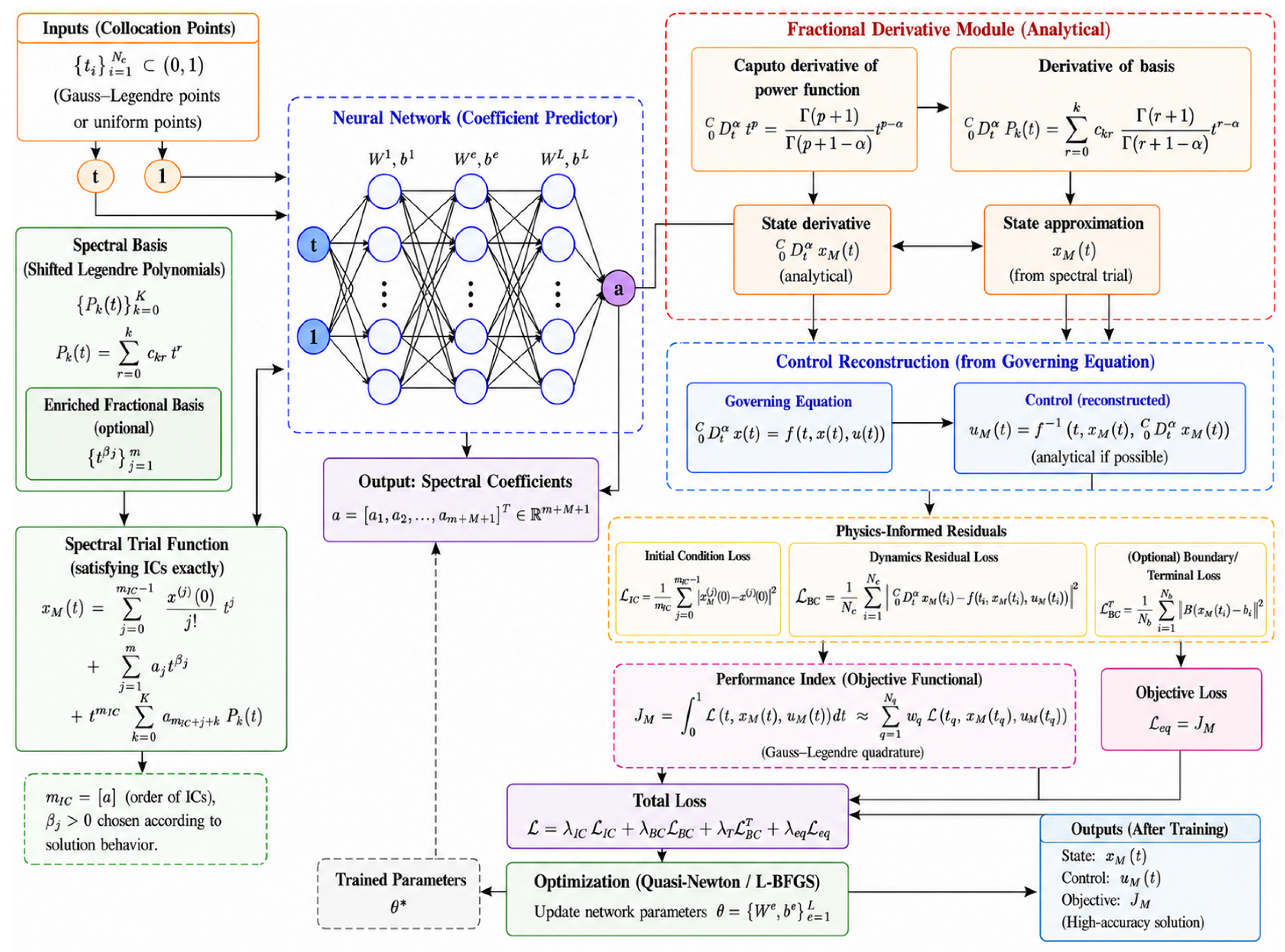
Figure 1 illustrates the overall computational workflow of the proposed Spectral-fPINN framework. The framework uses shifted Legendre spectral approximations in combination with physics-informed neural networks, where collocation points are passed first into a neural coefficient predictor to produce the trainable spectral coefficients for the state, control and adjoint variables. The coefficients are then used to construct the spectral trial solutions. The fractional derivative module computes the Caputo fractional derivatives with spectral operational matrices. The optimality-system residuals guarantee the state equation, the adjoint equation and the stationarity condition. The objective functional and residual equations are integrated using Gauss–Legendre quadrature and added to the total physics-informed loss function. The resulting optimization problem is solved iteratively using gradient-based optimization algorithms. Unlike conventional PINN architectures that directly approximate the unknown solution variables using fully connected neural networks, the present framework predicts the spectral coefficients associated with the shifted Legendre basis functions. This spectral representation greatly enhances the approximation accuracy and the convergence behavior for smooth solutions, and simultaneously reduces the number of trainable parameters. The proposed architecture consists of several modules. First, collocation points are generated across the computational domain and passed to the neural coefficient predictor. The input layer generates collocation points firstly distributed across the computational domain. These collocation points are then fed into the neural coefficient predictor, which computes the trainable spectral coefficients for the state, control and adjoint variables. These coefficients are used to construct the spectral trial solutions based on shifted Legendre polynomial expansions. The fractional derivative module then computes the Caputo fractional derivatives using spectral operational matrix formulations. These derivatives are then incorporated into the fractional optimality system to construct the residual functions associated with the state equation, adjoint equation, and stationarity condition. The resulting residuals are directly incorporated into the physics-informed loss function, together with the objective functional and the prescribed initial and boundary conditions.

Finally, the total loss function is minimized iteratively using optimization algorithms such as quasi-Newton or L-BFGS methods until convergence. After training, the optimized spectral coefficients are used to reconstruct the approximate solutions of the state, control and adjoint of the fractional optimal control problem. Therefore, the proposed Spectral-fPINN architecture leverages the high-order approximation capabilities of spectral methods and the flexibility of physics-informed neural networks, leading to an efficient and highly accurate computational framework for solving general fractional optimal control systems. The pseudocode of the proposed method is presented in Algorithm 1.

Algorithm 1 Spectral-fPINN Framework for Fractional Optimal Control Problems

Input:       Fractional optimal control problem on $[t_0,t_f]$       Fractional order $\alpha$, spectral order N       Gauss–Legendre quadrature rule ${\{t_q,{\omega }_q\}}_{q=1}^{N_q}$       Penalty sequence ${\left\{{\rho }_k\right\}}_{k=1}^s$       Neural network architecture and optimization parameters   Output:       Approximate state $x_N\left(t\right)$, control $u_N\left(t\right)$, costate ${\lambda }_N\left(t\right)$, objective value ${\mathcal{J}}_N$ 1:  Construct the normalized shifted Legendre basis and the corresponding fractional operational matrices. 2:  Initialize the neural network parameters using Xavier initialization. Since a single problem instance is considered, the network input is taken as a fixed constant. 3:  Represent the state, control, and costate variables through shifted Legendre spectral expansions with trainable coefficient vectors. 4:  for $k=1,\dots ,s$ do 5:     Set the penalty parameter $\rho ={\rho }_k$. 6:     for $epoch=1,\dots ,N_{\max }$ do 7:        Predict the spectral coefficients using the neural network. 8:        Reconstruct the approximate state, control, and costate functions. 9:        Evaluate the Caputo fractional derivatives using the operational matrix formulation. 10:       Construct the residuals of the state equation, adjoint equation, and stationarity condition. 11:       Evaluate the discrete objective functional using Gauss–Legendre quadrature. 12:       Form the total loss function $$\mathcal{L}={\mathcal{L}}_J+{\mathcal{L}}_{\mathrm{res}}+{\mathcal{L}}_{\mathrm{IC}}+{\mathcal{L}}_{\mathrm{TC}}.$$ 13:      Here, ${\mathcal{L}}_J$ is the quadrature-approximated objective, ${\mathcal{L}}_{\mathrm{res}}$ is the penalized residual loss, and ${\mathcal{L}}_{\mathrm{IC}}$ and ${\mathcal{L}}_{\mathrm{TC}}$ are the boundary loss terms. 14:      Compute the gradient of $\mathcal{L}$ using automatic differentiation. 15:      Update the neural network parameters using Adam or L-BFGS. 16:      if $\mathcal{L}<{\epsilon }_{\mathcal{L}}$ or $\parallel {\nabla }_{\theta }{\mathcal{L}\parallel }_2<{\epsilon }_g$ then 17:          break 18:      end if 19:    end for 20:    Use the optimized parameters as the initial guess for the next continuation stage. 21: end for 22: Reconstruct the final approximate solution from the optimized spectral coefficients. 23: Compute residual norms and spectral coefficient decay to assess convergence and accuracy. 24: Return $x_N\left(t\right)$, $u_N\left(t\right)$, ${\lambda }_N\left(t\right)$, and ${\mathcal{J}}_N$.

4. Theoretical Analysis of the Spectral-fPINN Framework

In this section, we provide a theoretical justification for the proposed Spectral-fPINN methodology. The analysis focuses on the approximation properties of the shifted Legendre basis, consistency of the fractional operational matrix formulation, residual consistency of the optimality system, spectral convergence, stability of the residual formulation, and optimization convergence of the proposed framework.

4.1. Approximation Properties of the Spectral Representation

The proposed Spectral-fPINN framework approximates the state, control, and adjoint variables through the normalized shifted Legendre expansions

$$x_N\left(t\right)={\mathsf{\Psi }}_x\left(t\right)+{\mathcal{B}}_x\left(t\right){\displaystyle \sum _{j=0}^N}{a}_j{\widehat{\mathsf{\Phi }}}_j\left(t\right),$$

$$u_N\left(t\right)={\displaystyle \sum _{j=0}^N}{b}_j{\widehat{\mathsf{\Phi }}}_j\left(t\right),$$

and

$${\lambda }_N\left(t\right)={\mathsf{\Psi }}_{\lambda }\left(t\right)+{\mathcal{B}}_{\lambda }\left(t\right){\displaystyle \sum _{j=0}^N}{c}_j{\widehat{\mathsf{\Phi }}}_j\left(t\right),$$

where the auxiliary functions ${\mathsf{\Psi }}_x\left(t\right)$, ${\mathsf{\Psi }}_{\lambda }\left(t\right)$, ${\mathcal{B}}_x\left(t\right)$, and ${\mathcal{B}}_{\lambda }\left(t\right)$ are selected so that the prescribed initial and terminal conditions are satisfied exactly.

Theorem 1

(Approximation Theorem). Suppose that

$$x,u,\lambda \in H^m(0,1),m\ge 1.$$

Then there exist coefficient vectors ${\mathbf{a}}^{*},{\mathbf{b}}^{*},{\mathbf{c}}^{*}$ such that

$$\parallel x-x_N{\parallel }_{L^2(0,1)}+\parallel u-u_N{\parallel }_{L^2(0,1)}+{\parallel \lambda -{\lambda }_N\parallel }_{L^2(0,1)}\le C{N}^{-m},$$

where $C>0$ is independent of N. Furthermore, if the exact solutions are analytic on $[0,1]$, then

$$\parallel x-x_N{\parallel }_{L^2(0,1)}+\parallel u-u_N{\parallel }_{L^2(0,1)}+{\parallel \lambda -{\lambda }_N\parallel }_{L^2(0,1)}\le C{e}^{-\sigma N},$$

for some constants $C,\sigma >0$.

Proof. 

Let

$${\mathbb{P}}_N=\mathrm{span}\{{\widehat{\mathsf{\Phi }}}_0,{\widehat{\mathsf{\Phi }}}_1,\dots ,{\widehat{\mathsf{\Phi }}}_N\}$$

be the normalized shifted Legendre polynomial space of degree at most N, and let

$${\mathsf{\Pi }}_N:L^2(0,1)\to {\mathbb{P}}_N$$

denote the corresponding $L^2$-orthogonal projection.

For any $f\in H^m(0,1)$, standard spectral approximation theory yields

$$\parallel f-{\mathsf{\Pi }}_N{f\parallel }_{L^2(0,1)}\le C_f{N}^{-m}{\parallel f\parallel }_{H^m(0,1)}.$$

Applying this estimate to x, u, and $\lambda$, and choosing the spectral coefficients corresponding to their orthogonal projections onto ${\mathbb{P}}_N$, we obtain

$$\parallel x-x_N{\parallel }_{L^2(0,1)}+\parallel u-u_N{\parallel }_{L^2(0,1)}+{\parallel \lambda -{\lambda }_N\parallel }_{L^2(0,1)}\le C{N}^{-m},$$

for some constant $C>0$.

If x, u, and $\lambda$ are analytic on $[0,1]$, then standard spectral convergence theory implies exponential decay of the normalized shifted Legendre coefficients. Consequently, there exist constants $C,\sigma >0$ such that

$$\parallel x-x_N{\parallel }_{L^2(0,1)}+\parallel u-u_N{\parallel }_{L^2(0,1)}+{\parallel \lambda -{\lambda }_N\parallel }_{L^2(0,1)}\le C{e}^{-\sigma N}.$$

This completes the proof. □

4.2. Consistency of the Fractional Operational Matrix

The Caputo fractional derivatives are approximated by

$${}_{t_0}{}^C\mathcal{D}_t^{\alpha }{x}_N\left(t\right)={}_{t_0}{}^C\mathcal{D}_t^{\alpha }{\mathsf{\Psi }}_x\left(t\right)+{\mathbf{a}}^{\mathsf{T}}{\mathbf{D}}^{\left(\alpha \right)}\mathbf{\Phi }\left(t\right),$$

and

$${}_t{}^C\mathcal{D}_{t_f}^{\alpha }{\lambda }_N\left(t\right)={}_t{}^C\mathcal{D}_{t_f}^{\alpha }{\mathsf{\Psi }}_{\lambda }\left(t\right)+{\mathbf{c}}^{\mathsf{T}}{\tilde{\mathbf{D}}}^{\left(\alpha \right)}\mathbf{\Phi }\left(t\right),$$

where

$$\mathbf{\Phi }\left(t\right)={\left[{\widehat{\mathsf{\Phi }}}_0\left(t\right),{\widehat{\mathsf{\Phi }}}_1\left(t\right),\dots ,{\widehat{\mathsf{\Phi }}}_N\left(t\right)\right]}^{\mathsf{T}},$$

and ${\mathbf{D}}^{\left(\alpha \right)}$ and ${\tilde{\mathbf{D}}}^{\left(\alpha \right)}$ denote the operational matrices corresponding to the left- and right-sided Caputo derivatives, respectively.

The matrices are obtained by projecting the fractional derivatives of the normalized shifted Legendre basis functions onto the same basis:

$${}_{t_0}{}^C\mathcal{D}_t^{\alpha }{\widehat{\mathsf{\Phi }}}_j\left(t\right)={\displaystyle \sum _{i=0}^N}{D}_{ij}^{\left(\alpha \right)}{\widehat{\mathsf{\Phi }}}_i\left(t\right)+{\tau }_{j,N}\left(t\right),$$

where ${\tau }_{j,N}\left(t\right)$ denotes the truncation error. For analytic functions, ${\tau }_{j,N}\left(t\right)$ decays exponentially with N, whereas algebraic decay is obtained for finite regularity.

Theorem 2

(Operational Matrix Consistency). Let $f\in H^m(0,1)$ with $m\ge \alpha$, and let $f_N$ be its normalized shifted Legendre projection of degree N. Then

$$\underset{N\to \infty }{\lim }{∥{}_{t_0}{}^C\mathcal{D}_t^{\alpha }f-{}_{t_0}{}^C\mathcal{D}_t^{\alpha }{f}_N∥}_{L^2(0,1)}=0.$$

Moreover, the operational matrix approximation is consistent, i.e.,

$${\tau }_{j,N}\to 0,N\to \infty ,$$

in the appropriate norm.

Proof. 

Let

$$e_N\left(t\right)=f\left(t\right)-f_N\left(t\right).$$

By linearity of the Caputo derivative,

$${}_{t_0}{}^C\mathcal{D}_t^{\alpha }f-{}_{t_0}{}^C\mathcal{D}_t^{\alpha }{f}_N={}_{t_0}{}^C\mathcal{D}_t^{\alpha }{e}_N.$$

Since the Caputo derivative is a bounded linear operator from $H^{\alpha }(0,1)$ into $L^2(0,1)$, there exists a constant $C_{\alpha }>0$ such that

$${∥{}_{t_0}{}^C\mathcal{D}_t^{\alpha }{e}_N∥}_{L^2(0,1)}\le C_{\alpha }{\parallel e_N\parallel }_{H^{\alpha }(0,1)}.$$

Because $f_N$ is the normalized shifted Legendre projection of f, standard spectral approximation theory implies

$$\parallel e_N{\parallel }_{H^{\alpha }(0,1)}\to 0,N\to \infty ,$$

which proves

$${∥{}_{t_0}{}^C\mathcal{D}_t^{\alpha }f-{}_{t_0}{}^C\mathcal{D}_t^{\alpha }{f}_N∥}_{L^2(0,1)}\to 0.$$

The operational matrix approximation introduces only the truncation error ${\tau }_{j,N}$, which vanishes as $N\to \infty$. Therefore, the matrix representation converges to the exact fractional derivative and remains consistent. □

4.3. Residual Consistency Analysis

The residual functions associated with the fractional optimality system (20)–(22) are defined by

$${\mathcal{R}}_1\left(t\right)={}_{t_0}{}^C\mathcal{D}_t^{\alpha }{x}_N\left(t\right)-{\displaystyle \frac{\partial \mathcal{H}}{\partial \lambda }},$$

$${\mathcal{R}}_2\left(t\right)={}_t{}^C\mathcal{D}_{t_f}^{\alpha }{\lambda }_N\left(t\right)+{\displaystyle \frac{\partial \mathcal{H}}{\partial x}},$$

and

$${\mathcal{R}}_3\left(t\right)={\displaystyle \frac{\partial \mathcal{H}}{\partial u}}.$$

Theorem 3

(Residual Consistency). Assume that the exact solution $(x,u,\lambda )$ satisfies the fractional optimality system (20)–(22). Let

$$x_N\to x,u_N\to u,{\lambda }_N\to \lambda$$

in $L^2(0,1)$, and suppose that

$${}_{t_0}{}^C\mathcal{D}_t^{\alpha }{x}_N\to {}_{t_0}{}^C\mathcal{D}_t^{\alpha }x,{}_t{}^C\mathcal{D}_{t_f}^{\alpha }{\lambda }_N\to {}_t{}^C\mathcal{D}_{t_f}^{\alpha }\lambda$$

in $L^2(0,1)$. Then

$$\parallel {\mathcal{R}}_i{\parallel }_{L^2(0,1)}\to 0,i=1,2,3.$$

Hence, the proposed Spectral-fPINN formulation is consistent with the continuous fractional optimality system.

Proof. 

Since the exact solution satisfies the fractional optimality system,

$${}_{t_0}{}^C\mathcal{D}_t^{\alpha }x={\displaystyle \frac{\partial \mathcal{H}}{\partial \lambda }},{}_t{}^C\mathcal{D}_{t_f}^{\alpha }\lambda =-{\displaystyle \frac{\partial \mathcal{H}}{\partial x}},{\displaystyle \frac{\partial \mathcal{H}}{\partial u}}=0.$$

For the state residual,

$$\begin{array}{cc}\hfill \parallel {\mathcal{R}}_1{\parallel }_{L^2(0,1)}& \le {∥{}_{t_0}{}^C\mathcal{D}_t^{\alpha }{x}_N-{}_{t_0}{}^C\mathcal{D}_t^{\alpha }x∥}_{L^2(0,1)}\hfill \\ & +{∥{\displaystyle \frac{\partial \mathcal{H}}{\partial \lambda }}(t,x_N,u_N,{\lambda }_N)-{\displaystyle \frac{\partial \mathcal{H}}{\partial \lambda }}(t,x,u,\lambda )∥}_{L^2(0,1)}.\hfill \end{array}$$

The first term tends to zero by assumption, while the second term tends to zero by the continuity of $\partial \mathcal{H}/\partial \lambda$. Therefore,

$$\parallel {\mathcal{R}}_1{\parallel }_{L^2(0,1)}\to 0.$$

The proof for ${\mathcal{R}}_2$ is analogous and yields

$$\parallel {\mathcal{R}}_2{\parallel }_{L^2(0,1)}\to 0.$$

Similarly, since

$${\displaystyle \frac{\partial \mathcal{H}}{\partial u}}(t,x,u,\lambda )=0,$$

we have

$${\mathcal{R}}_3\left(t\right)={\displaystyle \frac{\partial \mathcal{H}}{\partial u}}(t,x_N,u_N,{\lambda }_N)-{\displaystyle \frac{\partial \mathcal{H}}{\partial u}}(t,x,u,\lambda ).$$

By the convergence of $(x_N,u_N,{\lambda }_N)$ and the continuity of $\partial \mathcal{H}/\partial u$, it follows that

$$\parallel {\mathcal{R}}_3{\parallel }_{L^2(0,1)}\to 0.$$

Consequently,

$$\parallel {\mathcal{R}}_i{\parallel }_{L^2(0,1)}\to 0,i=1,2,3,$$

which proves the residual consistency of the proposed Spectral-fPINN formulation. □

4.4. Spectral Convergence Analysis

The convergence rate of the proposed Spectral-fPINN framework is determined by the decay of the normalized shifted Legendre coefficients.

Theorem 4

(Spectral Convergence). Suppose that the exact state, control, and adjoint variables are analytic on $[0,1]$. Then there exist constants $C>0$ and $\sigma >0$ such that

$$\parallel x-x_N{\parallel }_{L^2(0,1)}+\parallel u-u_N{\parallel }_{L^2(0,1)}+{\parallel \lambda -{\lambda }_N\parallel }_{L^2(0,1)}\le C{e}^{-\sigma N}.$$

Moreover,

$$\parallel {\mathcal{R}}_i{\parallel }_{L^2(0,1)}=\mathcal{O}\left(e^{-\sigma N}\right),i=1,2,3.$$

Proof. 

Since x, u, and $\lambda$ are analytic on $[0,1]$, standard spectral approximation theory implies exponential decay of their normalized shifted Legendre coefficients. Consequently, there exist constants $C,\sigma >0$ such that

$$\parallel x-x_N{\parallel }_{L^2(0,1)}+\parallel u-u_N{\parallel }_{L^2(0,1)}+{\parallel \lambda -{\lambda }_N\parallel }_{L^2(0,1)}\le C{e}^{-\sigma N}.$$

From the residual definitions and the fact that the exact solution satisfies the fractional optimality system, we have

$$\parallel {\mathcal{R}}_i{\parallel }_{L^2(0,1)}\le K_i\left(\parallel x-x_N{\parallel }_{L^2(0,1)}+\parallel u-u_N{\parallel }_{L^2(0,1)}+{\parallel \lambda -{\lambda }_N\parallel }_{L^2(0,1)}\right),$$

for some constants $K_i>0$, $i=1,2,3$. Therefore,

$$\parallel {\mathcal{R}}_i{\parallel }_{L^2(0,1)}=\mathcal{O}\left(e^{-\sigma N}\right),i=1,2,3.$$

This completes the proof. □

Remark 1.

If the exact solution possesses only finite regularity,

$$x,u,\lambda \in H^m(0,1),m\ge 1,$$

then the convergence rate becomes algebraic:

$$\parallel x-x_N{\parallel }_{L^2(0,1)}+\parallel u-u_N{\parallel }_{L^2(0,1)}+{\parallel \lambda -{\lambda }_N\parallel }_{L^2(0,1)}=\mathcal{O}\left(N^{-m}\right).$$

4.5. Stability of the Residual Formulation

Define

$$U=(x,u,\lambda ),\tilde{U}=(\tilde{x},\tilde{u},\tilde{\lambda }),$$

and let

$$\mathcal{R}\left(U\right)=({\mathcal{R}}_1,{\mathcal{R}}_2,{\mathcal{R}}_3)$$

denote the residual operator.

Theorem 5

(Residual Stability). Assume that the Hamiltonian

$$\mathcal{H}(t,x,u,\lambda )$$

is continuously differentiable and that its partial derivatives are Lipschitz continuous with respect to $(x,u,\lambda )$. Then there exists a constant $K>0$ such that

$$\parallel \mathcal{R}\left(U\right)-\mathcal{R}\left(\tilde{U}\right){\parallel }_{L^2(0,1)}\le K{\parallel U-\tilde{U}\parallel }_{H^{\alpha }(0,1)}.$$

Consequently, small perturbations in the spectral coefficients produce proportionally small perturbations in the residual functions.

Proof. 

From the residual definitions, the differences

$${\mathcal{R}}_i\left(U\right)-{\mathcal{R}}_i\left(\tilde{U}\right),i=1,2,3,$$

consist of Caputo derivative terms and Hamiltonian derivatives. By continuity of the Caputo derivative operator and the Lipschitz continuity of the Hamiltonian derivatives, there exist constants $K_i>0$ such that

$$\parallel {\mathcal{R}}_i\left(U\right)-{\mathcal{R}}_i\left(\tilde{U}\right){\parallel }_{L^2(0,1)}\le K_i{\parallel U-\tilde{U}\parallel }_{H^{\alpha }(0,1)},i=1,2,3.$$

Summing the above inequalities and setting

$$K=K_1+K_2+K_3,$$

yields

$$\parallel \mathcal{R}\left(U\right)-\mathcal{R}\left(\tilde{U}\right){\parallel }_{L^2(0,1)}\le K{\parallel U-\tilde{U}\parallel }_{H^{\alpha }(0,1)}.$$

This completes the proof. □

4.6. Error Estimate and Residual Control

The approximation, consistency, stability, and spectral convergence results established in Theorems 1–4 provide a theoretical justification for the accuracy of the proposed Spectral-fPINN framework.

Let

$$U=(x,u,\lambda ),U_N=(x_N,u_N,{\lambda }_N),$$

and define

$$\parallel U-U_N{\parallel }_{L^2(0,1)}:=\parallel x-x_N{\parallel }_{L^2(0,1)}+\parallel u-u_N{\parallel }_{L^2(0,1)}+{\parallel \lambda -{\lambda }_N\parallel }_{L^2(0,1)}.$$

The total approximation error is governed by two sources: the truncation error of the finite-dimensional normalized shifted Legendre approximation and the residual error associated with the approximate satisfaction of the fractional optimality system. Consequently, the overall numerical accuracy depends jointly on the convergence of the spectral approximation and the decay of the residual vector

$$\mathcal{R}\left(U_N\right)=({\mathcal{R}}_1,{\mathcal{R}}_2,{\mathcal{R}}_3).$$

For solutions with finite regularity,

$$x,u,\lambda \in H^m(0,1),m\ge 1,$$

Theorem 1 yields the algebraic estimate

$$\parallel U-U_N{\parallel }_{L^2(0,1)}=\mathcal{O}\left(N^{-m}\right).$$

For analytic solutions, Theorem 4 gives the stronger exponential estimate

$$\parallel U-U_N{\parallel }_{L^2(0,1)}=\mathcal{O}\left(e^{-\sigma N}\right),$$

for some constant $\sigma >0$.

Moreover, by Theorem 3,

$$\parallel {\mathcal{R}}_i{\parallel }_{L^2(0,1)}\to 0,i=1,2,3.$$

Therefore, as the residual loss decreases and the spectral order N increases, the approximate solution converges to the exact solution of the continuous fractional optimality system.

4.7. Optimization Convergence Discussion

The total loss function of the proposed Spectral-fPINN framework is defined by

$$\mathcal{L}\left(\theta \right)={\mathcal{L}}_J+{\mathcal{L}}_{\mathrm{res}}+{\mathcal{L}}_{\mathrm{IC}}+{\mathcal{L}}_{\mathrm{TC}},$$

where $\theta$ denotes the trainable parameters of the coefficient-prediction network. Since the normalized shifted Legendre expansions, Hamiltonian function, activation function $\tanh (·)$, and Gauss–Legendre quadrature are continuously differentiable, the discrete loss function $\mathcal{L}\left(\theta \right)$ is smooth with respect to $\theta$. The optimization is performed using the L-BFGS algorithm. Under standard smoothness assumptions, any accumulation point ${\theta }^{*}$ of the generated iterates satisfies the first-order stationarity condition

$${\nabla }_{\theta }\mathcal{L}\left({\theta }^{*}\right)=0.$$

Because the optimization problem is generally non-convex, global convergence cannot be guaranteed theoretically. Nevertheless, the numerical experiments reported in this work consistently exhibit stable convergence toward stationary solutions with negligible residual errors. To improve robustness, a continuation strategy is employed for the penalty parameter $\rho$. Starting from a relatively small value, $\rho$ is gradually increased through several optimization stages, while the optimized parameters from the previous stage are used as the initial guess for the subsequent stage. This strategy improves the enforcement of the fractional optimality system and enhances the stability of the optimization process.

5. Results and Discussion

The proposed Spectral-fPINN framework is tested on several benchmark fractional optimal control problems to investigate its accuracy, stability, and computational efficiency. The numerical performance is assessed through error measurements, residual evaluations, spectral coefficient decay, and graphical comparisons with the corresponding analytical solutions.

5.1. Example 1

We first consider a classical integer-order optimal control problem corresponding to the limiting case $\alpha =1$. Although the governing equation does not explicitly involve a fractional derivative, this example serves as a benchmark for validating the accuracy, stability, and consistency of the proposed Spectral-fPINN framework before applying it to genuinely fractional optimal control problems.

Consider the following optimal control problem:

$$\min J={\displaystyle \frac{1}{2}}{\int }_0^1\left(x^2\left(t\right)+u^2\left(t\right)\right)dt,$$

subject to

$${\displaystyle \frac{dx\left(t\right)}{dt}}=-x\left(t\right)+u\left(t\right),x\left(0\right)=1.$$

The exact solution is given by

$$x\left(t\right)=\cosh \left(\sqrt{2}t\right)+\beta \sinh \left(\sqrt{2}t\right),$$

$$u\left(t\right)=(1+\sqrt{2}\beta )\cosh \left(\sqrt{2}t\right)+(\sqrt{2}+\beta )\sinh \left(\sqrt{2}t\right),$$

where

$$\beta =-{\displaystyle \frac{\cosh \left(\sqrt{2}\right)+\sqrt{2}\sinh \left(\sqrt{2}\right)}{\sqrt{2}\cosh \left(\sqrt{2}\right)+\sinh \left(\sqrt{2}\right)}}.$$

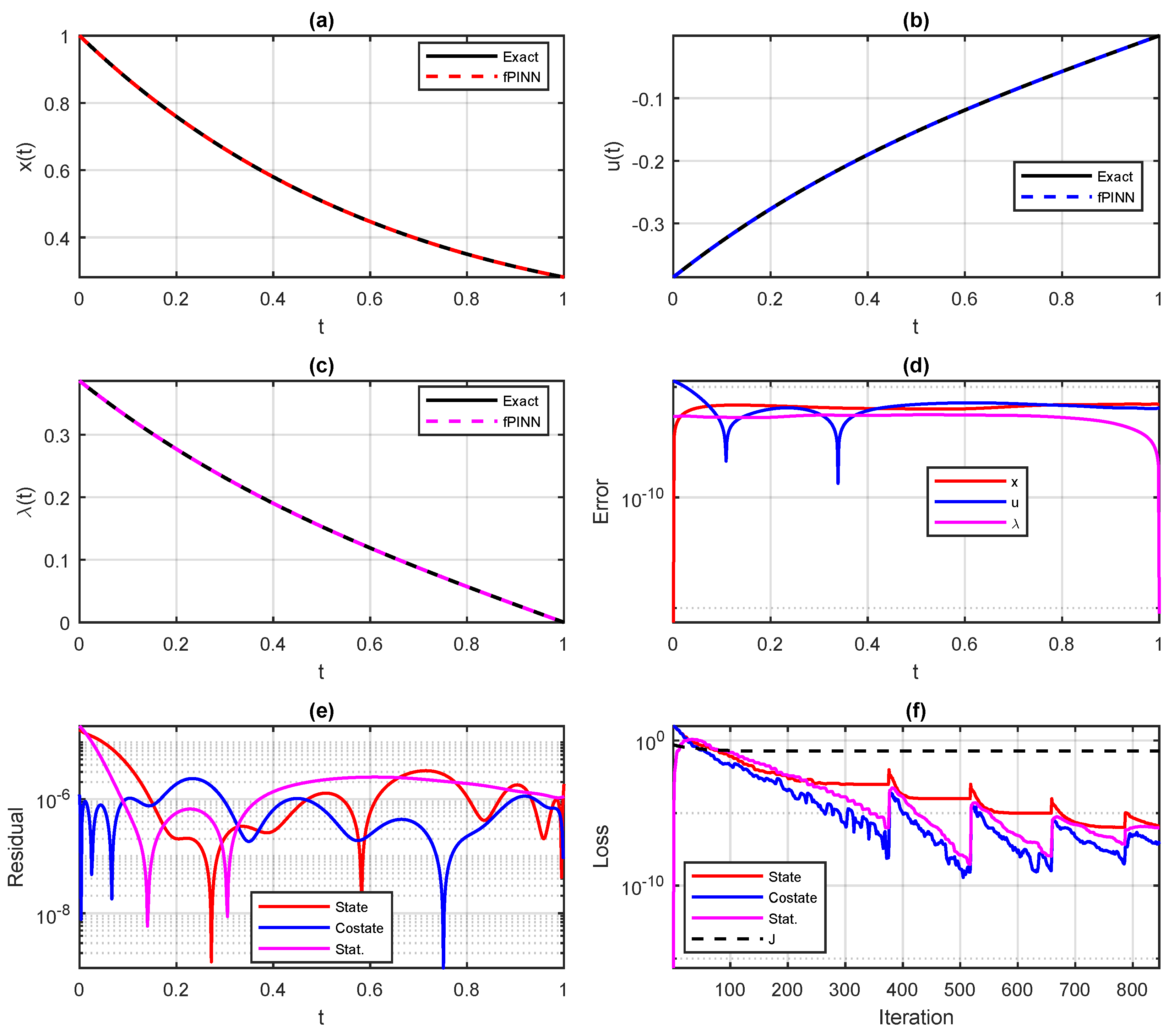
The corresponding exact objective value is $J_{\mathrm{exact}}=0.192909298100000$. We employ the proposed Spectral-fPINN framework to solve this problem using normalized shifted Legendre polynomial approximations together with physics-informed optimization. The numerical results are summarized in

Table 1. Training loss values for Example 1 using different penalty parameters.

Penalty Parameter ${\mathit{\lambda }}_{\mathit{r}}$	Loss Value
${10}^1$	$1.919336914469989\times {10}^{-1}$
${10}^2$	$1.928109692116326\times {10}^{-1}$
${10}^3$	$1.928994730466952\times {10}^{-1}$
${10}^4$	$1.929084288415424\times {10}^{-1}$
${10}^5$	$1.929111691877855\times {10}^{-1}$

and

Table 2. Numerical accuracy of the optimality-system spectral-fPINN method for Example 1.

Quantity	Value
Approximate cost functional J	$0.192908884539428$
Exact cost functional $J_{\mathrm{exact}}$	$0.192909298100000$
Absolute error in J	$4.1356\times {10}^{-7}$
Maximum error in $x\left(t\right)$	$1.6610\times {10}^{-6}$
Maximum error in $u\left(t\right)$	$1.8731\times {10}^{-5}$
Maximum error in $\lambda \left(t\right)$	$5.5023\times {10}^{-7}$
State residual $L^2$ error	$3.5564\times {10}^{-6}$
Costate residual $L^2$ error	$8.8035\times {10}^{-7}$
Stationarity residual $L^2$ error	$3.0698\times {10}^{-6}$

and the corresponding state, control and costate approximations are presented in Figure 2. The reported errors are calculated on an independent set of test points and provide a measure for the actual approximation errors with respect to the analytical solution. The residual quantities represent the degree to which the computed solution satisfies the governing optimality system.

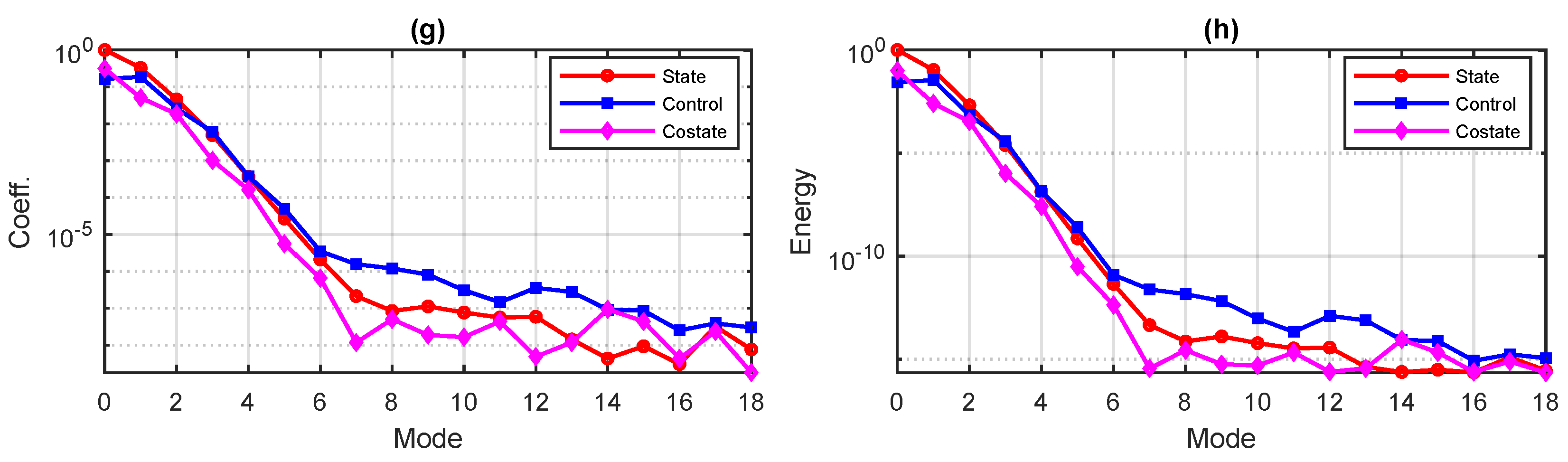
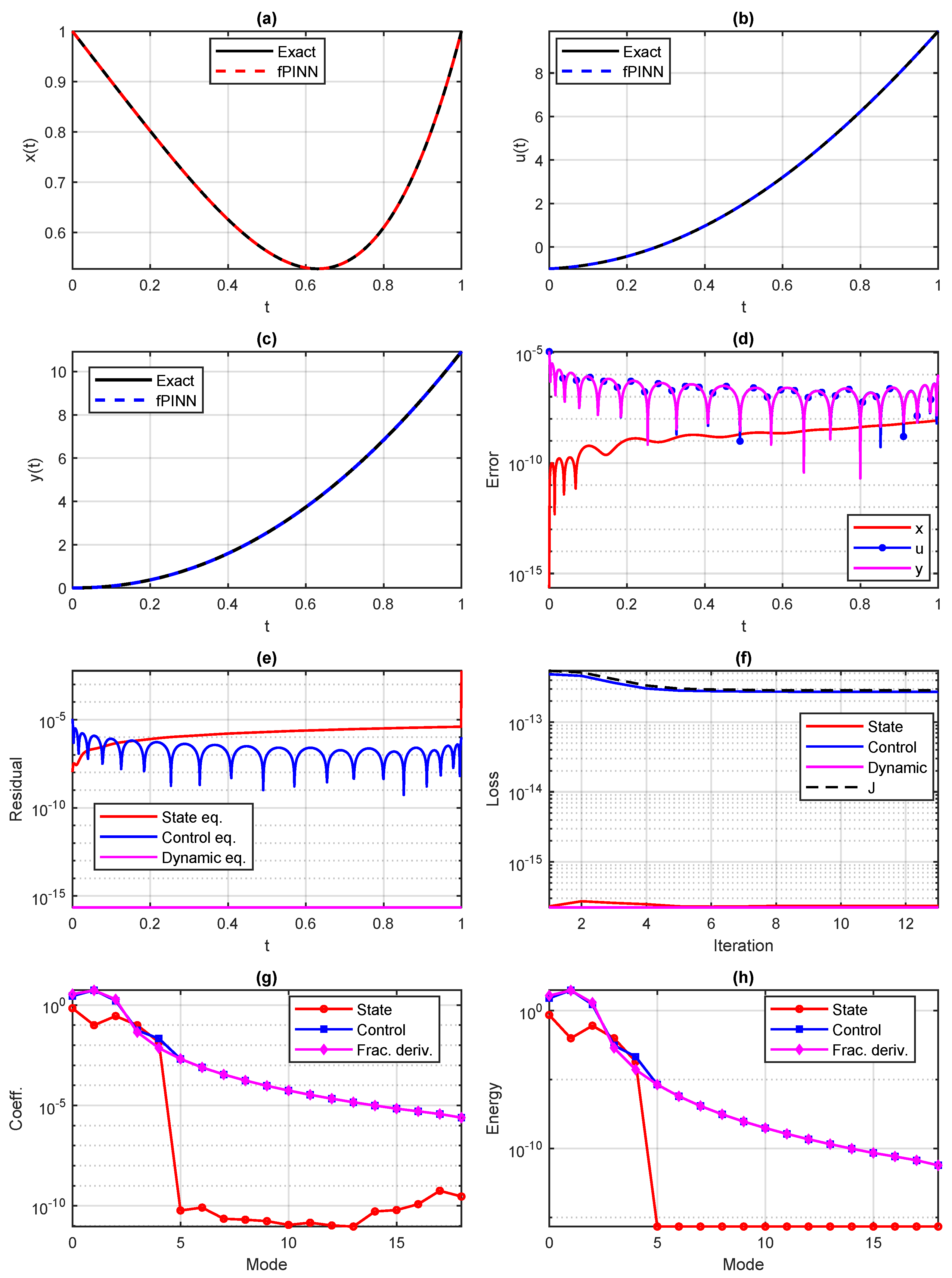
The numerical results presented in Table 1 and Table 2 demonstrate that the proposed Spectral-fPINN framework yields highly accurate approximations for the state, control and costate variables. The computed objective functional is in good agreement with the exact value with an absolute error of order ${10}^{-7}$. Furthermore, the residual norms for the state equation, costate equation and stationarity condition are small, which implies that the computed solution satisfies the optimality system accurately. Figure 2a–c displays the exact and approximate state, control and costate variables respectively, with excellent agreement over the computational interval. The pointwise absolute errors in Figure 2d are uniformly small and the residual profiles in Figure 2e remain close to zero in the whole domain. The evolution of loss components is depicted in Figure 2f, showing a stable convergence of the optimization process. Moreover, the fast decay of the spectral coefficients in Figure 2g and the spectral energy distributions in Figure 2h confirm the high-order accuracy, compactness and computational efficiency of the normalized shifted Legendre representation.

Overall, this example demonstrates that the proposed Spectral-fPINN framework provides a reliable and accurate approach for solving optimal control problems and serves as a solid foundation for the subsequent fractional-order examples.

5.2. Example 2

In this example, we consider a fractional optimal control problem involving a Caputo fractional derivative of order $\alpha =1.1$ in order to assess the ability of the proposed Spectral-fPINN framework to accurately approximate fractional dynamics and optimal control variables.

Consider

$$\min J={\int }_0^1\left[{\left(x\left(t\right)-t^2\right)}^2+{\left(u\left(t\right)+t^4-{\displaystyle \frac{20}{9\Gamma (9/10)}}{t}^{9/10}\right)}^2\right]dt,$$

subject to

$${}_0{}^{C}D_t^{1.1}x\left(t\right)=t^{2}x\left(t\right)+u\left(t\right).$$

The exact solutions are

$$x\left(t\right)=t^2,$$

$$u\left(t\right)={\displaystyle \frac{20}{9\Gamma (9/10)}}{t}^{9/10}-t^4,$$

and

$$y\left(t\right)={}_0{}^{C}D_t^{1.1}x\left(t\right)={\displaystyle \frac{20}{9\Gamma (9/10)}}{t}^{9/10}.$$

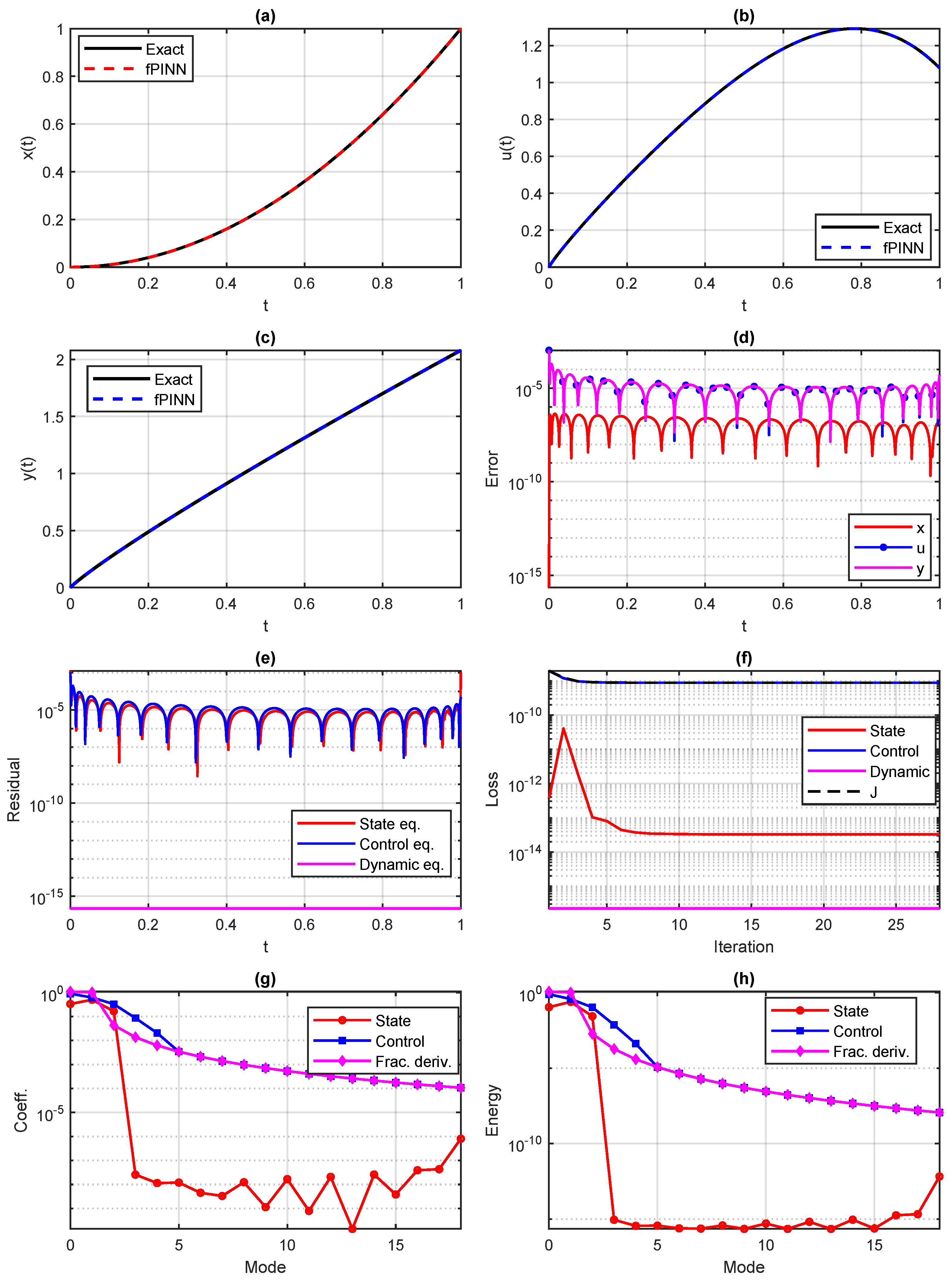
The proposed Spectral-fPINN framework is employed using normalized shifted Legendre polynomial approximations together with physics-informed optimization. The numerical results are summarized in

Table 3. Training loss values for Example 2 using different penalty parameters.

Penalty Parameter ${\mathit{\lambda }}_{\mathit{r}}$	Loss Value
${10}^1$	$8.865345834759386\times {10}^{-10}$
${10}^2$	$8.865345823898574\times {10}^{-10}$
${10}^3$	$8.865345823898574\times {10}^{-10}$
${10}^4$	$8.865345823898574\times {10}^{-10}$
${10}^5$	$8.865345823898574\times {10}^{-10}$

and

Table 4. Numerical accuracy of the spectral-fPINN method for Example 2.

Quantity	Value
Approximate cost functional J	$8.865345823898574\times {10}^{-10}$
Exact cost functional $J_{\mathrm{exact}}$	0
Absolute error in J	$8.8653\times {10}^{-10}$
Maximum error in $x\left(t\right)$	$4.2909\times {10}^{-7}$
Maximum error in $u\left(t\right)$	$1.0519\times {10}^{-3}$
Maximum error in $y\left(t\right)$	$1.0519\times {10}^{-3}$
State residual $L^2$ error	$1.8008\times {10}^{-7}$
Control residual $L^2$ error	$2.9774\times {10}^{-5}$
Dynamic residual $L^2$ error	0

, while Figure 3 presents the corresponding state, control, and fractional derivative approximations. The reported errors are computed using an independent set of test points and measure the actual approximation errors with respect to the analytical solutions, whereas the residual quantities assess the satisfaction of the governing fractional optimality system.

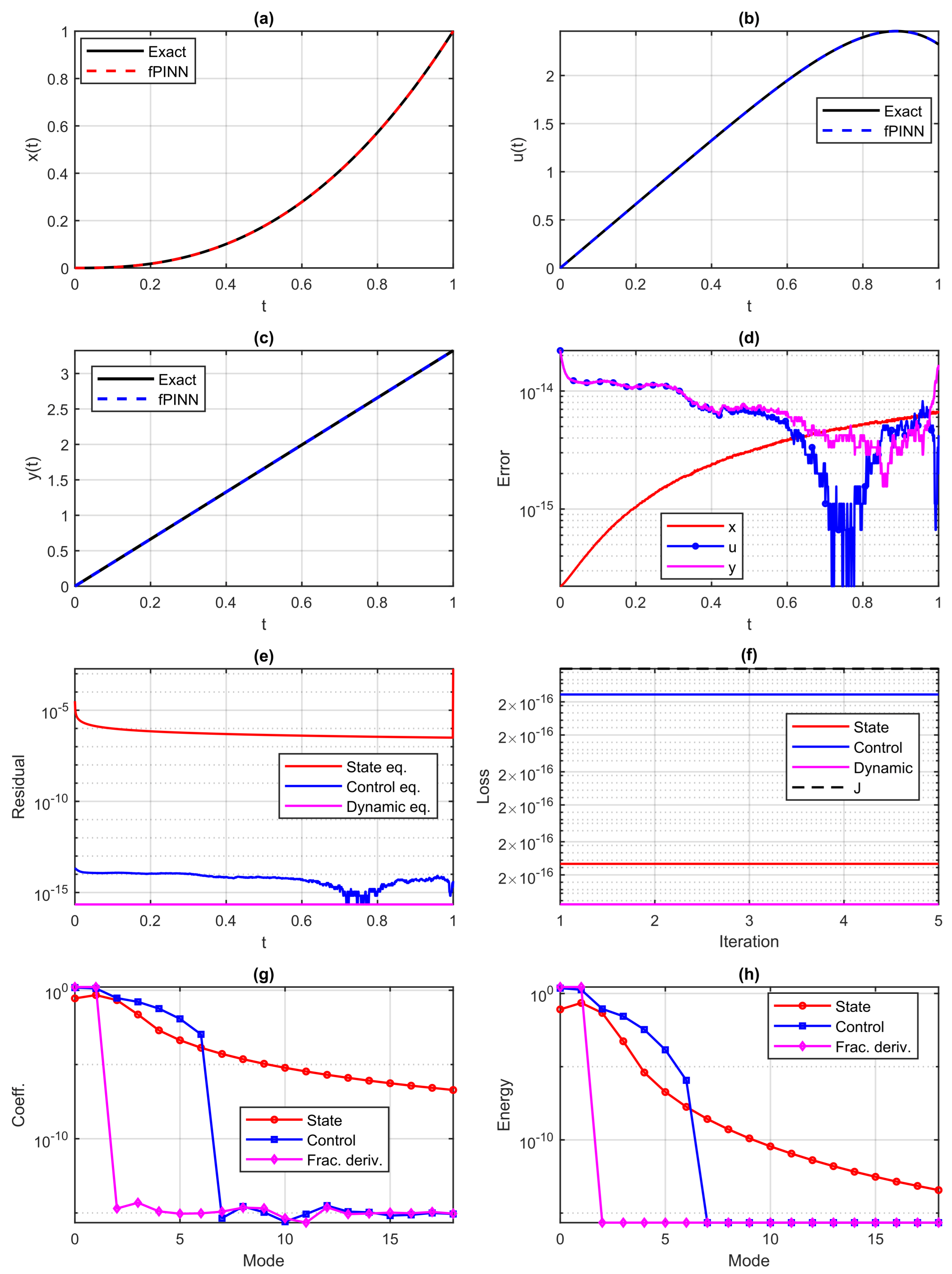
The numerical results reported in Table 3 and Table 4 show that the proposed Spectral-fPINN framework yields highly accurate approximations for the state, control and fractional derivative variables. The computed objective functional matches very well the exact value with an absolute error of order ${10}^{-10}$. The residual norms are also small, which verifies that the computed solution satisfies the governing fractional optimality system with high accuracy. Moreover, the training history shows stable optimization behavior with the increase in the penalty parameter. Figure 3a–c presents the comparison of the exact and approximate state, control and fractional derivative variables, respectively. In all cases, the numerical solutions are in excellent agreement with the respective analytical solutions over the entire computational interval. The pointwise absolute errors in Figure 3d are uniformly small, which confirms the high approximation accuracy and spectral convergence of the proposed method. The residual errors corresponding to the governing equations are shown in Figure 3e.

It is observed that the residual errors are close to zero in the entire domain. The evolution of the loss components shown in Figure 3f suggests that the optimization process converges stably. The fast decay of the spectral coefficients in Figure 3g indicates the high-order approximation capability of the normalized shifted Legendre basis, and the spectral energy distributions in Figure 3h demonstrate that most of the solution energy is concentrated in the lower-order modes. These observations confirm the computational efficiency and compactness of the proposed spectral representation.

Overall, this example demonstrates that the proposed Spectral-fPINN framework provides an accurate, stable, and computationally efficient approach for solving fractional optimal control problems involving fractional-order dynamical systems.

5.3. Example 3

In this example, we consider a fractional optimal control problem involving a higher-order Caputo derivative of order $\alpha =1.9$. This example assesses the ability of the proposed Spectral-fPINN framework to approximate higher-order fractional dynamics and the corresponding optimal control variables.

Consider

$$\min J={\int }_0^1\left[e^t{\left(x\left(t\right)-t^4+t-1\right)}^2+(1+t^2){\left(u\left(t\right)+1-t+t^4-{\displaystyle \frac{8000}{77\Gamma (1/10)}}{t}^{21/10}\right)}^2\right]dt,$$

subject to

$${}_0{}^{C}D_t^{1.9}x\left(t\right)=x\left(t\right)+u\left(t\right).$$

The exact solutions are

$$x\left(t\right)=t^4-t+1,$$

$$u\left(t\right)=-1+t-t^4+{\displaystyle \frac{8000}{77\Gamma (1/10)}}{t}^{21/10},$$

and

$$y\left(t\right)={}_0{}^{C}D_t^{1.9}x\left(t\right)={\displaystyle \frac{8000}{77\Gamma (1/10)}}{t}^{21/10}.$$

Hence, the exact objective value is $J_{\mathrm{exact}}=0$.

The proposed Spectral-fPINN framework is applied using normalized shifted Legendre polynomial approximations and physics-informed optimization. The numerical results are summarized in

Table 5. Training loss values for Example 3 using different penalty parameters.

Penalty Parameter ${\mathit{\lambda }}_{\mathit{r}}$	Loss Value
${10}^1$	$2.850001935471632\times {10}^{-13}$
${10}^2$	$2.850001935471632\times {10}^{-13}$
${10}^3$	$2.850001935471632\times {10}^{-13}$
${10}^4$	$2.850001935471632\times {10}^{-13}$
${10}^5$	$2.850001935471632\times {10}^{-13}$

and

Table 6. Numerical accuracy of the spectral-fPINN method for Example 3.

Quantity	Value
Approximate cost functional J	$2.850001935471632\times {10}^{-13}$
Exact cost functional $J_{\mathrm{exact}}$	0
Absolute error in J	$2.8500\times {10}^{-13}$
Maximum error in $x\left(t\right)$	$8.3823\times {10}^{-9}$
Maximum error in $u\left(t\right)$	$1.1012\times {10}^{-5}$
Maximum error in $y\left(t\right)$	$1.1012\times {10}^{-5}$
State residual $L^2$ error	$3.2787\times {10}^{-9}$
Control residual $L^2$ error	$5.2170\times {10}^{-7}$
Dynamic residual $L^2$ error	0

, while Figure 4 presents the corresponding graphical comparisons. The reported errors are evaluated on an independent set of test points with respect to the analytical solutions, whereas the residual quantities measure the satisfaction of the governing fractional optimality system.

The numerical results reported in Table 5 and Table 6 demonstrate that the proposed Spectral-fPINN framework provides highly accurate approximations for this higher-order fractional optimal control problem. The computed objective functional is in excellent agreement with the exact value, with an absolute error of order ${10}^{-13}$. The residual norms are also small, confirming that the computed solution satisfies the governing fractional optimality system with high accuracy. Furthermore, the training history exhibits stable optimization behavior as the penalty parameter increases. Figure 4a–c compares the exact and approximate state, control, and fractional derivative variables, respectively. In all cases, the numerical solutions closely match the corresponding analytical solutions throughout the computational interval, demonstrating the ability of the proposed framework to accurately capture higher-order fractional dynamics. The pointwise absolute errors shown in Figure 4d remain uniformly small, confirming the high approximation accuracy and spectral convergence of the method.

The residual errors shown in Figure 4e are also close to zero over the entire computational domain, providing further evidence that the computed solution indeed satisfies the governing fractional optimality system. The evolution of the loss components in Figure 4f shows the stable convergence of the optimization process. Moreover, the fast decay of the spectral coefficients, as shown in Figure 4g, reveals the high-order approximation capability of the normalized shifted Legendre basis. The distributions of the spectral energy in Figure 4h show that most of the solution energy is concentrated in the low-order modes. These observations confirm the compactness and computational efficiency of the proposed spectral representation.

Overall, this example demonstrates that the proposed Spectral-fPINN framework provides an accurate, stable and computationally efficient approach for solving fractional optimal control problems involving higher-order fractional dynamics.

5.4. Example 4

In this example, we consider a nonlinear fractional optimal control problem involving a Caputo derivative of order $\alpha =1.5$. This example is intended to assess the ability of the proposed Spectral-fPINN framework to solve nonlinear fractional optimal control problems with smooth analytical solutions.

Consider

$$\min J={\int }_0^1\left[{\left(x\left(t\right)-t^{5/2}\right)}^4+(1+t^2){\left(u\left(t\right)+t^6-{\displaystyle \frac{15\sqrt{\pi }}{8}}t\right)}^2\right]dt,$$

subject to

$${}_0{}^{C}D_t^{1.5}x\left(t\right)=t{x}^2\left(t\right)+u\left(t\right).$$

The exact solutions are

$$x\left(t\right)=t^{5/2},$$

$$u\left(t\right)={\displaystyle \frac{15\sqrt{\pi }}{8}}t-t^6,$$

and

$$y\left(t\right)={}_0{}^{C}D_t^{1.5}x\left(t\right)={\displaystyle \frac{15\sqrt{\pi }}{8}}t.$$

Hence, the exact objective value is

$$J_{\mathrm{exact}}=0.$$

The proposed Spectral-fPINN framework is employed using normalized shifted Legendre polynomial approximations together with physics-informed optimization. The numerical results are summarized in

Table 7. Training loss values for Example 4 using different penalty parameters.

Penalty Parameter ${\mathit{\lambda }}_{\mathit{r}}$	Loss Value
${10}^1$	$6.747545425453489\times {10}^{-29}$
${10}^2$	$6.747545425453489\times {10}^{-29}$
${10}^3$	$6.747545425453489\times {10}^{-29}$
${10}^4$	$6.747545425453489\times {10}^{-29}$
${10}^5$	$6.747545425453489\times {10}^{-29}$

and

Table 8. Numerical accuracy of the spectral-fPINN method for Example 4.

Quantity	Value
Approximate cost functional J	$6.747545425453489\times {10}^{-29}$
Exact cost functional $J_{\mathrm{exact}}$	0
Absolute error in J	$6.7475\times {10}^{-29}$
Maximum error in $x\left(t\right)$	$6.4393\times {10}^{-15}$
Maximum error in $u\left(t\right)$	$2.1786\times {10}^{-14}$
Maximum error in $y\left(t\right)$	$2.1786\times {10}^{-14}$
State residual $L^2$ error	$3.5082\times {10}^{-15}$
Control residual $L^2$ error	$7.7477\times {10}^{-15}$
Dynamic residual $L^2$ error	0

, while Figure 5 presents the corresponding graphical comparisons. The reported errors are evaluated on an independent set of test points with respect to the analytical solutions, whereas the residual quantities measure the satisfaction of the governing nonlinear fractional optimality system.

The numerical results in Table 7 and Table 8 show that the proposed Spectral-fPINN framework can produce very accurate approximations for this nonlinear fractional optimal control problem. The computed objective functional is very close to the exact value and the residual norms are small, which confirms that the computed solution is a high accuracy solution of the governing nonlinear fractional optimality system. Moreover, the training history indicates stable optimization behavior for the increasing penalty parameter. The comparison of the exact and approximate variables of the state, control and fractional derivative are shown in Figure 5a–c. The numerical solutions in all cases are in good agreement with the corresponding analytical solutions over the computational interval, which demonstrates the ability of the proposed framework to capture nonlinear fractional dynamics accurately. The pointwise absolute errors in Figure 5d are uniformly small, which further verifies the high approximation accuracy and spectral convergence of the method.

Finally, the residual errors shown in Figure 5e remain uniformly close to zero throughout the computational domain, further validating that the computed solution satisfies the governing fractional optimality system. The evolution of the loss components in Figure 5f indicates a stable convergence of the optimization process. Moreover, the fast decay of the spectral coefficients displayed in Figure 5g indicates that the normalized shifted Legendre basis has the high-order approximation capability. The spectral energy distributions in Figure 5h show that most of the solution energy is concentrated in the lower-order modes. These results verify the compactness and computational efficiency of the proposed spectral representation.

Overall, this example demonstrates that the proposed Spectral-fPINN framework provides an accurate, stable, and computationally efficient approach for solving nonlinear fractional optimal control problems. The conditioning of the fractional operational matrices generally deteriorates as the spectral order N increases, which is a common feature of global spectral discretizations. In the present work, moderate values of N are employed, and the numerical experiments demonstrate stable convergence without noticeable loss of accuracy. For very large spectral orders, preconditioning and matrix-scaling strategies may be beneficial to further improve numerical robustness.

All numerical experiments were performed in MATLAB R2023b using double-precision arithmetic. The Spectral-fPINN framework employs a fully connected feed-forward neural network with four hidden layers and 40 neurons per hidden layer. The hyperbolic tangent activation function is used throughout the hidden layers. Network parameters are initialized using the Xavier (Glorot) initialization strategy. The trainable parameters are optimized using the Adam optimizer with an initial learning rate of ${10}^{-3}$, combined with an exponential learning-rate decay strategy. Full-batch training is employed, where all Gauss–Legendre collocation points are used simultaneously in the loss evaluation. The optimization process is terminated when either the loss function becomes smaller than ${10}^{-12}$ or the gradient norm falls below ${10}^{-10}$. No additional regularization techniques are applied. For all numerical examples, a penalty continuation strategy is adopted using

$${\lambda }_r\in \{{10}^1,{10}^2,{10}^3,{10}^4,{10}^5\},$$

where the optimized parameters obtained at one penalty level are used as the initial guess for the subsequent level. All computations were performed on a 64-bit Windows workstation equipped with an Intel Core i7-1255U processor, 16 GB RAM, and an NVIDIA GeForce RTX 2050 GPU.

6. Conclusions

In this work, a corrected Spectral-fPINN framework based on normalized shifted Legendre polynomial approximations and operational matrices of fractional differentiation has been developed for solving fractional optimal control problems. The proposed methodology combines the high-order accuracy of spectral methods with the flexibility of physics-informed optimization. Both the theoretical analysis and numerical experiments demonstrate the accuracy, stability, consistency, and spectral convergence properties of the proposed framework. The numerical results show highly accurate approximations together with very small residual errors, confirming the effectiveness of the method for a variety of linear and nonlinear fractional optimal control problems. The theoretical results establish approximation, consistency, stability, and convergence properties of the proposed framework, while the numerical experiments verify these findings through several benchmark problems. In addition, the observed rapid decay of spectral coefficients and residual norms confirms the strong approximation capability of the normalized shifted Legendre representation within the proposed Spectral-fPINN framework. The proposed framework has potential applications in a wide range of areas, including engineering systems with memory effects, anomalous diffusion and transport processes in physics, biological systems exhibiting hereditary behavior, and optimal control of fractional-order dynamical systems. The flexibility and high-order accuracy of the proposed methodology make it a promising computational tool for solving practical problems governed by fractional differential equations. The proposed framework is particularly suitable for smooth fractional optimal control problems, where spectral approximations achieve rapid convergence. However, for problems involving discontinuities or nonsmooth solutions, additional adaptive techniques may be required. Furthermore, the computational cost may increase for large-scale multidimensional systems. Future work will focus on constrained, variable-order, and multidimensional fractional optimal control problems, as well as adaptive Spectral-fPINN formulations for more complex applications.

References

1. Podlubny, I. Fractional Differential Equations; Academic Press: New York, NY, USA, 1999. [Google Scholar]
2. Kilbas, A.A.; Srivastava, H.M.; Trujillo, J.J. Theory and Applications of Fractional Differential Equations; Elsevier: Amsterdam, The Netherlands, 2006. [Google Scholar]
3. Samko, S.G.; Kilbas, A.A.; Marichev, O.I. Fractional Integrals and Derivatives: Theory and Applications; Gordon and Breach Science Publishers: Yverdon, Switzerland, 1993. [Google Scholar]
4. Magin, R.L. Fractional Calculus in Bioengineering. Crit. Rev. Biomed. Eng. 2004, 32, 1–104. [Google Scholar] [CrossRef] [Scilit] [PubMed]
5. Benson, D.A.; Wheatcraft, S.W.; Meerschaert, M.M. Application of a Fractional Advection–Dispersion Equation. Water Resour. Res. 2000, 36, 1403–1412. [Google Scholar] [CrossRef] [Scilit]
6. Diethelm, K. The Analysis of Fractional Differential Equations; Springer: Berlin/Heidelberg, Germany, 2010. [Google Scholar] [CrossRef] [Scilit]
7. Vazquez, J.L. The Mathematical Theories of Diffusion: Nonlinear and Fractional Diffusion. In Fractional Dynamics; Klages, R., Radons, G., Sokolov, I.M., Eds.; Springer: Cham, Switzerland, 2017; pp. 205–278. [Google Scholar] [CrossRef] [Scilit]
8. Chen, W.; Holm, S. Fractional Laplacian time-space models for linear and nonlinear lossy media exhibiting arbitrary frequency power-law dependency. J. Acoust. Soc. Am. 2004, 115, 1424–1430. [Google Scholar] [CrossRef] [Scilit] [PubMed]
9. Sun, H.; Zhang, Y.; Chen, W.; Reeves, D.M. Use of a variable-index fractional-derivative model to capture transient dispersion in heterogeneous media. J. Contam. Hydrol. 2014, 157, 47–58. [Google Scholar] [CrossRef] [Scilit] [PubMed]
10. Agrawal, O.P.; Baleanu, D. A Hamiltonian Formulation and a Direct Numerical Scheme for Fractional Optimal Control Problems. J. Vib. Control 2007, 13, 1269–1281. [Google Scholar] [CrossRef] [Scilit]
11. Almeida, R.; Torres, D.F.M. Necessary and sufficient conditions for the fractional calculus of variations with Caputo derivatives. Commun. Nonlinear Sci. Numer. Simul. 2011, 16, 1490–1500. [Google Scholar] [CrossRef] [Scilit]
12. Kamocki, R. On the existence of optimal solutions to fractional optimal control problems. Appl. Math. Comput. 2014, 235, 94–104. [Google Scholar] [CrossRef] [Scilit]
13. Sakthivel, R.; Ren, Y.; Mahmudov, N.I. On the approximate controllability of semilinear fractional differential systems. Comput. Math. Appl. 2011, 62, 1451–1459. [Google Scholar] [CrossRef] [Scilit]
14. Mursaleen, A.M. Controllability of Tempered Caputo Fractional Dynamical Systems. J. Nonlinear Convex Anal. 2025, 26, 2501–2511. [Google Scholar]
15. Wu, J.; Xie, H.; Li, T.; He, W.; Xi, T.; Liang, X. Design of a Finite-Time Bounded Tracking Controller for Time-Delay Fractional-Order Systems Based on Output Feedback. Mathematics 2025, 13, 200. [Google Scholar] [CrossRef] [Scilit]
16. Liang, X.; Ge, S.S. Zone Barrier Lyapunov Functions for State Constrained Systems. IEEE Trans. Instrum. Meas. 2023, 72, 3001911. [Google Scholar] [CrossRef] [Scilit]
17. Liu, S.; Wang, J. Optimal Controls of Systems Governed by Semilinear Fractional Differential Equations with Not Instantaneous Impulses. J. Optim. Theory Appl. 2017, 174, 455–473. [Google Scholar] [CrossRef] [Scilit]
18. Lotfi, A.; Dehghan, M.; Yousefi, S.A. A numerical technique for solving fractional optimal control problems. Comput. Math. Appl. 2011, 62, 1055–1067. [Google Scholar] [CrossRef] [Scilit]
19. Lotfi, A.; Yousefi, S.A.; Dehghan, M. Numerical solution of a class of fractional optimal control problems via the Legendre orthonormal basis combined with the operational matrix and the Gauss quadrature rule. J. Comput. Appl. Math. 2013, 250, 143–160. [Google Scholar] [CrossRef] [Scilit]
20. Bhrawy, A.H.; Doha, E.H.; Tenreiro Machado, J.A.; Ezz-Eldien, S.S. An Efficient Numerical Scheme for Solving Multi-Dimensional Fractional Optimal Control Problems with a Quadratic Performance Index. Asian J. Control 2015, 17, 2389–2402. [Google Scholar] [CrossRef] [Scilit]
21. Heydari, M.H.; Razzaghi, M.; Zhagharian, S. Numerical solution of distributed-order fractional 2D optimal control problems using the Bernstein polynomials. Int. J. Syst. Sci. 2023, 54, 2253–2267. [Google Scholar] [CrossRef] [Scilit]
22. Dehestani, H.; Ordokhani, Y.; Razzaghi, M. A robust optimisation approach for the 2D-VO fractional optimal control problems. Int. J. Syst. Sci. 2025, 56, 347–362. [Google Scholar] [CrossRef] [Scilit]
23. Meerschaert, M.M.; Tadjeran, C. Finite difference approximations for fractional advection–dispersion flow equations. J. Comput. Appl. Math. 2004, 172, 65–77. [Google Scholar] [CrossRef] [Scilit]
24. Roop, J.P. Computational aspects of FEM approximation of fractional advection–dispersion equations on bounded domains in ℝ2. J. Comput. Appl. Math. 2006, 193, 243–268. [Google Scholar] [CrossRef] [Scilit]
25. Mao, Z.; Shen, J. Efficient spectral–Galerkin methods for fractional partial differential equations with variable coefficients. J. Comput. Phys. 2016, 307, 243–261. [Google Scholar] [CrossRef] [Scilit]
26. Gottlieb, D.; Orszag, S.A. Numerical Analysis of Spectral Methods: Theory and Applications; CBMS-NSF Regional Conference Series in Applied Mathematics; SIAM: Philadelphia, PA, USA, 1977. [Google Scholar] [CrossRef] [Scilit]
27. Shen, J. Efficient spectral-Galerkin method I: Direct solvers of second- and fourth-order equations using Legendre polynomials. SIAM J. Sci. Comput. 1994, 15, 1489–1505. [Google Scholar] [CrossRef] [Scilit]
28. Zhao, T. Efficient Spectral Collocation Method for Tempered Fractional Differential Equations. Fractal Fract. 2023, 7, 277. [Google Scholar] [CrossRef] [Scilit]
29. Sirignano, J.; Spiliopoulos, K. DGM: A deep learning algorithm for solving partial differential equations. J. Comput. Phys. 2018, 375, 1339–1364. [Google Scholar] [CrossRef] [Scilit]
30. Berg, J.; Nyström, K. A unified deep artificial neural network approach to partial differential equations in complex geometries. Neurocomputing 2018, 317, 28–41. [Google Scholar] [CrossRef] [Scilit]
31. Jagtap, A.; Karniadakis, G.E. Extended physics-informed neural networks (XPINNs): A generalized space-time domain decomposition based deep learning framework for nonlinear partial differential equations. Commun. Comput. Phys. 2020, 28, 2002–2041. [Google Scholar] [CrossRef] [Scilit]
32. Raissi, M.; Perdikaris, P.; Karniadakis, G.E. Physics-informed neural networks: A deep learning framework for solving forward and inverse problems involving nonlinear partial differential equations. J. Comput. Phys. 2019, 378, 686–707. [Google Scholar] [CrossRef] [Scilit]
33. Yu, J.; Lu, L.; Meng, X.; Karniadakis, G.E. Gradient-enhanced physics-informed neural networks for forward and inverse PDE problems. Comput. Methods Appl. Mech. Eng. 2022, 393, 114823. [Google Scholar] [CrossRef] [Scilit]
34. Pang, G.; Lu, L.; Karniadakis, G.E. fPINNs: Fractional Physics-Informed Neural Networks. SIAM J. Sci. Comput. 2019, 41, A2603–A2626. [Google Scholar] [CrossRef] [Scilit]
35. Guo, L.; Wu, H.; Yu, X.; Zhou, T. Monte Carlo fPINNs: Deep learning method for forward and inverse problems involving high dimensional fractional partial differential equations. Comput. Methods Appl. Mech. Eng. 2022, 400, 115523. [Google Scholar] [CrossRef] [Scilit]
36. Hou, J.; Ma, Z.; Ying, S.; Li, Y. HNS: An efficient Hermite neural solver for solving time-fractional partial differential equations. Chaos Solitons Fractals 2024, 181, 114637. [Google Scholar] [CrossRef] [Scilit]
37. Aghaei, A.A.; Moghaddam, M.M.; Parand, K. PINNIES: An efficient physics-informed neural network framework for integral operator problems. Comput. Phys. Commun. 2026, 327, 110255. [Google Scholar] [CrossRef] [Scilit]
38. Rao, N.; Shahzad, M.; Jha, N. Study of two dimensional α-modified Bernstein bi-variate operators. Filomat 2025, 39, 1509–1522. [Google Scholar] [CrossRef] [Scilit]
39. Rao, N.; Farid, M.; Jha, N.K. A study of (σ, μ)-Stancu-Schurer as a new generalization and approximations. J. Inequal. Appl. 2025, 2025, 104. [Google Scholar] [CrossRef] [Scilit]
40. Wang, S.; Zhang, H.; Jiang, X. Fractional physics-informed neural networks for time-fractional phase field models. Nonlinear Dyn. 2022, 110, 2715–2739. [Google Scholar] [CrossRef] [Scilit]
41. Mao, Z.; Jagtap, A.D.; Karniadakis, G.E. Physics-informed neural networks for high-speed flows. Comput. Methods Appl. Mech. Eng. 2020, 360, 112789. [Google Scholar] [CrossRef] [Scilit]
42. Barry-Straume, J.; Sarshar, A.; Popov, A.A.; Sandu, A. Physics-Informed Neural Networks for PDE-Constrained Optimization and Control. Commun. Appl. Math. Comput. 2025. [Google Scholar] [CrossRef] [Scilit]
43. Mowlavi, S.; Nabi, S. Optimal control of PDEs using physics-informed neural networks. J. Comput. Phys. 2023, 473, 111731. [Google Scholar] [CrossRef] [Scilit]
44. Zhang, T.; Zhang, D.; Shi, S.; Guo, Z. Spectral-fPINNs: Spectral method based fractional physics-informed neural networks for solving fractional partial differential equations. Nonlinear Dyn. 2025, 113, 12565–12588. [Google Scholar] [CrossRef] [Scilit]
Figure 1. Architecture of the proposed Spectral-fPINN framework for solving fractional optimal control problems.
Computation 14 00146 g001
Figure 2. Example 1: (a) Comparison between the exact and spectral-fPINN state solutions. (b) Comparison between the exact and spectral-fPINN control solutions. (c) Comparison between the exact and spectral-fPINN costate solutions. (d) Pointwise absolute errors of the state, control, and costate variables. (e) Residual errors associated with the optimality system. (f) Evolution of the physics-informed loss components during training. (g) Decay of the spectral coefficients for the state, control, and costate approximations. (h) Spectral energy distribution of the state, control, and costate variables.
Computation 14 00146 g002aComputation 14 00146 g002b
Figure 3. Example 2: (a) Comparison between the exact and spectral-fPINN state solutions. (b) Comparison between the exact and spectral-fPINN control solutions. (c) Comparison between the exact and spectral-fPINN fractional derivative solutions. (d) Pointwise absolute errors of the state, control, and fractional derivative variables. (e) Residual errors associated with the governing system. (f) Evolution of the physics-informed loss components during training. (g) Decay of the spectral coefficients for the state, control, and fractional derivative approximations. (h) Spectral energy distribution of the state, control, and fractional derivative approximations.
Computation 14 00146 g003
Figure 4. Example 3: (a) Comparison between the exact and spectral-fPINN state solutions. (b) Comparison between the exact and spectral-fPINN control solutions. (c) Comparison between the exact and spectral-fPINN fractional derivative solutions. (d) Pointwise absolute errors of the state, control, and fractional derivative variables. (e) Residual errors associated with the governing system. (f) Evolution of the physics-informed loss components during training. (g) Decay of the spectral coefficients for the state, control, and fractional derivative approximations. (h) Spectral energy distribution of the state, control, and fractional derivative approximations.
Computation 14 00146 g004
Figure 5. Example 4: (a) Comparison between the exact and spectral-fPINN state solutions. (b) Comparison between the exact and spectral-fPINN control solutions. (c) Comparison between the exact and spectral-fPINN fractional derivative solutions. (d) Pointwise absolute errors of the state, control, and fractional derivative variables. (e) Residual errors associated with the governing system. (f) Evolution of the physics-informed loss components during training. (g) Decay of the spectral coefficients for the state, control, and fractional derivative approximations. (h) Spectral energy distribution of the state, control, and fractional derivative approximations.
Computation 14 00146 g005