A Spectrum-Driven Hierarchical Learning Network for Aero-Engine Defect Segmentation

Abstract

Aero-engine defects often exhibit micro-scale and high-frequency characteristics under complex metallic textures, which makes precise segmentation difficult. Most existing pixel-level methods rely on spatial-domain modeling and lack frequency-domain decoupling. As a result, high-frequency details are easily hidden by low-frequency background information. In addition, repeated downsampling weakens the representation of fine-grained structures, leading to inaccurate boundary localization and limited robustness. To address these issues, a spectrum-driven hierarchical learning network is proposed for aero-engine defect segmentation. First, a dual-band spectral module is constructed using the discrete cosine transform to separate high-frequency and low-frequency components, providing stable and physically meaningful frequency-domain priors for the network. Second, a detail-guided module is designed where high-frequency features adaptively guide skip connections, compensating information loss during encoding and improving boundary recovery. Furthermore, a low-frequency-driven region-aware modeling module is developed. The internal defect regions, boundary areas, and background regions are modeled hierarchically. A dynamic hyper-kernel generation mechanism performs region-sensitive convolutional modeling, improving adaptation to complex structural variations. Extensive experiments on the Turbo19 and NEU-Seg datasets demonstrate that the proposed method produces accurate defect boundaries and achieves mIoU scores of 89.82% and 91.44%, improving over the second-best method by 5.22% and 4.42%, respectively.

1. Introduction

Aero-engines are the core components and power source of aircraft, and their operating condition is directly related to flight safety and maintenance reliability. During operation, engine components are exposed to high-temperature, high-pressure, and high-speed conditions for long periods, which can easily lead to surface defects such as cracks, scratches, and tearing. Therefore, timely inspection of aero-engines is essential for maintaining the normal operation of both the engine and the aircraft. Endoscopy has become an important tool for identifying potential defects inside the complex structures of aero-engines.

With the development of deep learning, defect segmentation methods have been successfully applied in various industrial scenarios and have gradually been introduced into endoscopic inspection tasks. Many mature studies have been reported in this field [1,2,3,4]. Nevertheless, in real aero-engine inspection scenarios, complex metallic texture backgrounds, micro-scale defect targets, and ambiguous boundaries still make it difficult for existing methods to achieve satisfactory background suppression, detail recovery, and stable feature representation [5,6].

At present, because industrial defects often show large scale variations and ambiguous boundaries, most studies focus on two directions: multi-scale feature fusion and boundary-enhanced feature learning. Multi-scale feature fusion improves the model’s ability to represent and detect defects of different sizes by integrating feature information from different levels or receptive fields [7,8,9]. Boundary-enhanced feature learning improves the localization accuracy and segmentation quality of defect edges by strengthening the feature response and discrimination ability around defect contours [10,11].

Although the above methods improve the model’s ability to perceive targets at different scales to some extent, most of them still rely mainly on spatial-domain information and make limited use of frequency-domain features. Frequency-domain representation can effectively separate detailed information from global structural information in images, which is important for distinguishing defects from the background. At the same time, existing methods usually assume that the feature distribution across image regions is relatively uniform. They lack the ability to model the significant differences among different regions. As a result, it is difficult to adapt to the complex structural variations among defect interiors, boundaries, and background areas.

However, the existing methods still suffer from the following problems:

• In aero-engine defect detection, defects often appear as high-frequency details and are easily disturbed by complex low-frequency backgrounds. However, existing methods do not explicitly decouple high-frequency and low-frequency information. As a result, the model is easily dominated by the main frequency components, and small defects cannot be represented in a stable way [5,12].
• Aero-engine defects usually have small sizes, elongated shapes, and ambiguous boundaries. During the multiple downsampling operations in the encoder, high-frequency detail information (such as crack edges and the contours of small scratches) can be easily weakened or lost. As a result, the decoder has limited ability to describe defect boundaries and small defects [13,14].
• The interior of defects, boundary regions, and background areas show significant differences in appearance, texture, and structure. Traditional segmentation networks usually apply unified parameters for modeling. Therefore, it is difficult to achieve both accurate defect localization and effective background suppression. In particular, false detections are likely to occur under complex metallic texture backgrounds [9,15].

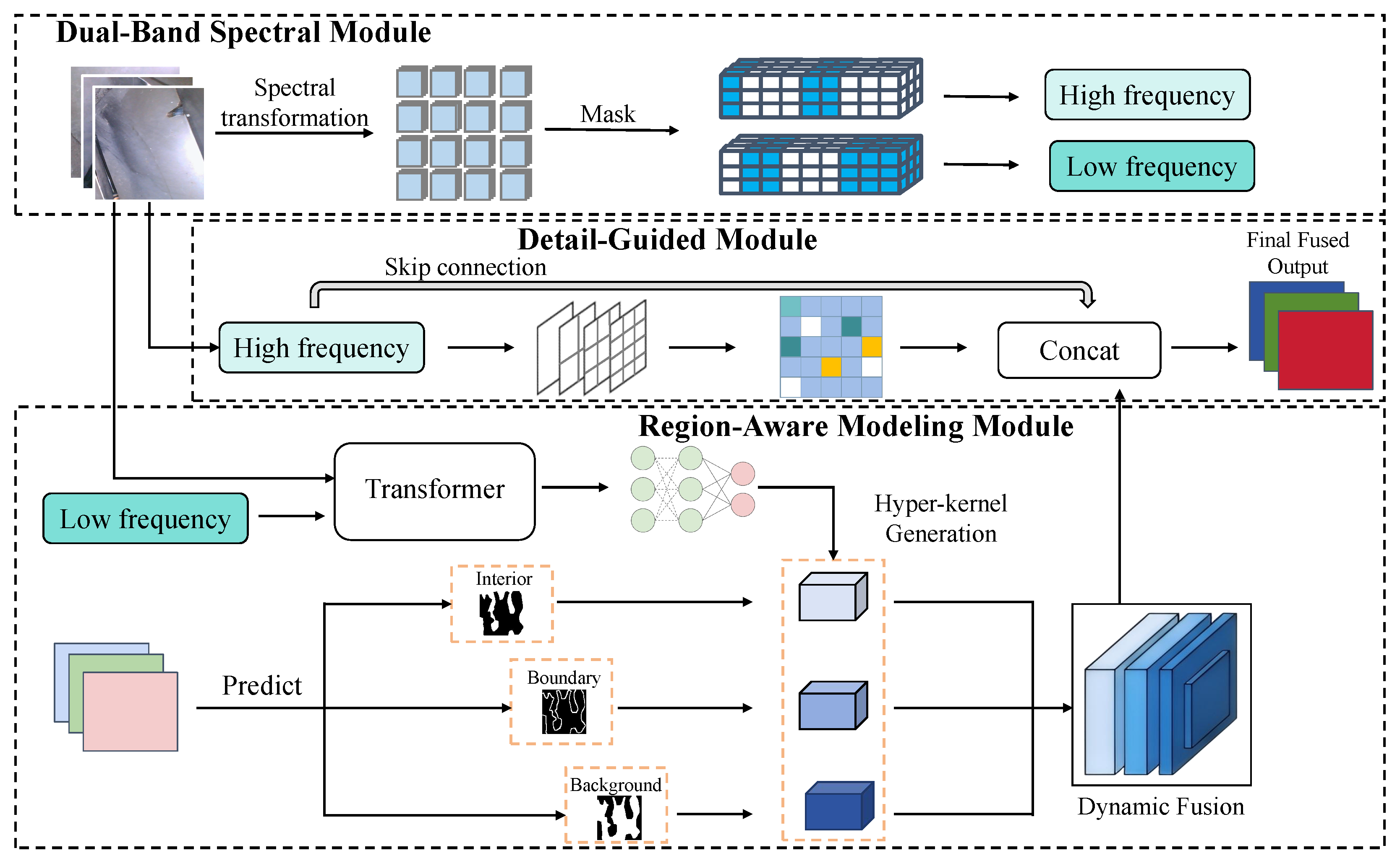
To address these issues, a novel hierarchical learning model is introduced for aero-engine defect segmentation. It consists of three key modules: a dual-band spectral module, a detail-guided module, and a region-aware modeling module. First, the dual-band spectral module maps the input image into the frequency domain through the discrete cosine transform, and the high-frequency and low-frequency components are explicitly separated. The high-frequency component mainly contains the edge and texture information of defects, while the low-frequency component reflects the global structure and background information of the image. Second, the detail-guided module uses high-frequency spectral features to generate guidance parameters. These parameters are used to adaptively guide the skip connection features produced by the encoder. In this way, the representation of defect-related details is strengthened, and fine structures are gradually recovered during the decoding process. Finally, the region-aware modeling module takes the low-frequency features as input. Region-level masks are generated, and region-sensitive branches are constructed to perform hierarchical modeling of the defect interior, boundary regions, and background areas. At the same time, a low-frequency-driven hyper-kernel generation mechanism dynamically provides region-sensitive convolution kernels for each decoding stage. This design allows the network to perform adaptive feature extraction according to the structural characteristics of different regions, thereby improving the model’s ability to handle complex appearance variations and different operating conditions.

The main contributions of this paper are summarized as follows:

• A dual-band spectral module is designed. The defect image is mapped into the frequency domain through the discrete cosine transform, and the frequency information is explicitly separated into high-frequency and low-frequency components. In this way, frequency-domain feature decoupling is achieved, and more discriminative frequency-domain feature representations are provided for the subsequent network [16,17].
• A detail-guided module is designed. Through skip connections, the spatial-domain feature maps are enhanced, and the information loss that is usually caused by downsampling is reduced [18,19].
• A region-aware modeling module is designed. The global structural stability contained in the low-frequency components is used as the basis for region modeling. The network is guided to adopt different modeling strategies for different regions, which significantly improves the localization accuracy and structural consistency of aero-engine defect detection in complex scenarios [20,21].

The rest of this paper is organized as follows. Section 2 describes the related work. Section 3 presents and details the proposed method. Section 4 reports and discusses the experimental results on two datasets to demonstrate the superiority of the proposed method. Finally, Section 5 provides the overall conclusions.

2. Related Work

This section reviews related studies from two aspects, namely aero-engine visual inspection and pixel-level defect segmentation, and analyzes their relevance and limitations for the task considered in this work.

2.1. Aero-Engine Visual Inspection

Advances in computer vision have promoted the transition from traditional visual inspection methods to deep learning-based aero-engine inspection techniques. Yang et al. [22] proposed a novel non-destructive defect detection network, NDD-Net, to build an end-to-end defect segmentation framework. The representation ability for micro-defects was enhanced through attention-based feature fusion and residual dense modeling. Tsai et al. [23] introduced a two-stage deep learning method that does not require manual annotation. Defect pixels were automatically synthesized and labeled using CycleGAN. The generated samples were then used to train U-Net to achieve pixel-level defect detection on textured surfaces. Xu et al. [24] proposed a defect detection system based on semantic segmentation. An end-to-end semantic segmentation network, Feature Pyramid Network–ResNet-34, was developed for defect detection, and experiments showed that the architecture is effective for defect feature extraction and fusion. Yang et al. [25] proposed an improved edge-guided and channel-enhanced network based on the Transformer architecture. Global edge information from Segment Anything Model was used to guide learning, while a channel shuffle module improved feature capture ability. Song et al. [26] designed a new feature extraction module based on Deformable Convolutional Networks. A deformable convolution structure was used to extract features from blades with different shapes. A channel attention module was also introduced so that the network could focus on surface anomalies. Utomo et al. [27] introduced R2U-Net, which systematically integrates residual connections to enhance gradient propagation. Recursive convolution units were used to refine contextual information for aero-engine blade defect detection. Liu et al. [28] proposed an improved detection algorithm based on YOLOv11. Context-guided large-kernel attention and a rotated detection head were introduced. Through dual structural optimization, both detection efficiency and accuracy were improved. Wang et al. [29] proposed a defect detection method for impeller blades based on three-dimensional point clouds. Computational complexity was reduced through point cloud segmentation and voxel downsampling. Multi-level local features such as normal vectors and Fast Point Feature Histogram were fused, and accurate recognition of scratch defects on complex impeller blades was achieved using Fuzzy C-Means Clustering. Although these methods have achieved considerable success, the variation in the shapes of segmentation targets limits their direct application to our task.

2.2. Pixel-Level Defect Segmentation

Pixel-level defect segmentation refers to the classification of each pixel in an image so that defect regions can be precisely distinguished from background regions and their contours can be accurately described. Yang et al. [30] proposed an end-to-end pixel-level defect segmentation network based on an encoder–decoder architecture. A residual attention backbone was used to enhance the feature representation of target regions, and a bidirectional ConvLSTM module was introduced to optimize skip connections and learn long-range spatial context. Zuo et al. [31] proposed a pixel-level defect segmentation network that integrates multi-scale features, global mapping, and attention mechanisms to improve the detection and segmentation of defects with different sizes. Qi et al. [32] proposed a one-click interactive defect segmentation method. User clicks were encoded as superpixel-guided Gaussian heat maps and embedded into the network for modeling. Combined with a customized backbone network and a Bayesian optimization refinement strategy, efficient and accurate segmentation of complex defects was achieved. Meng et al. [33] proposed a pixel-level defect detection method based on Mask R-CNN. Attention-based feature fusion and an improved classifier head were introduced to effectively suppress background interference and improve defect segmentation accuracy. Qi et al. [34] introduced an innovative semi-supervised defect segmentation method. In this framework, three parallel self-supervised mechanisms were integrated with a semi-supervised learning framework to improve defect semantic segmentation using limited labeled samples. Zhang et al. [35] proposed an adaptive feature refinement network based on U-Net. A pretrained EfficientNet-B0 was used as the encoder, and an AFR module was introduced to enhance channel and spatial feature modeling, enabling fine pixel-level segmentation of surface defects. Ma et al. [36] proposed a semantic prior-guided defect-aware network. Through collaborative modeling of semantic prior mining, defect-enhanced perception, and global information extraction modules, precise perception and efficient detection of small defects under complex backgrounds were achieved. Sun et al. [37] proposed a pixel-level tire defect detection method based on a lightweight Transformer. A dual-path encoder and a multi-scale spatial cross-transformer decoder were used to model both local and global pixel dependencies. Although these methods have achieved considerable success, existing pixel-level defect segmentation approaches still show limitations in frequency-domain feature decoupling and in preserving fine details that are often lost during downsampling.

3. Materials

This section introduces the materials used in this study, including the aero-engine endoscopic inspection system, the self-collected Turbo19 dataset, and the public NEU-Seg dataset.

3.1. Aero-Engine Endoscopic Inspection System

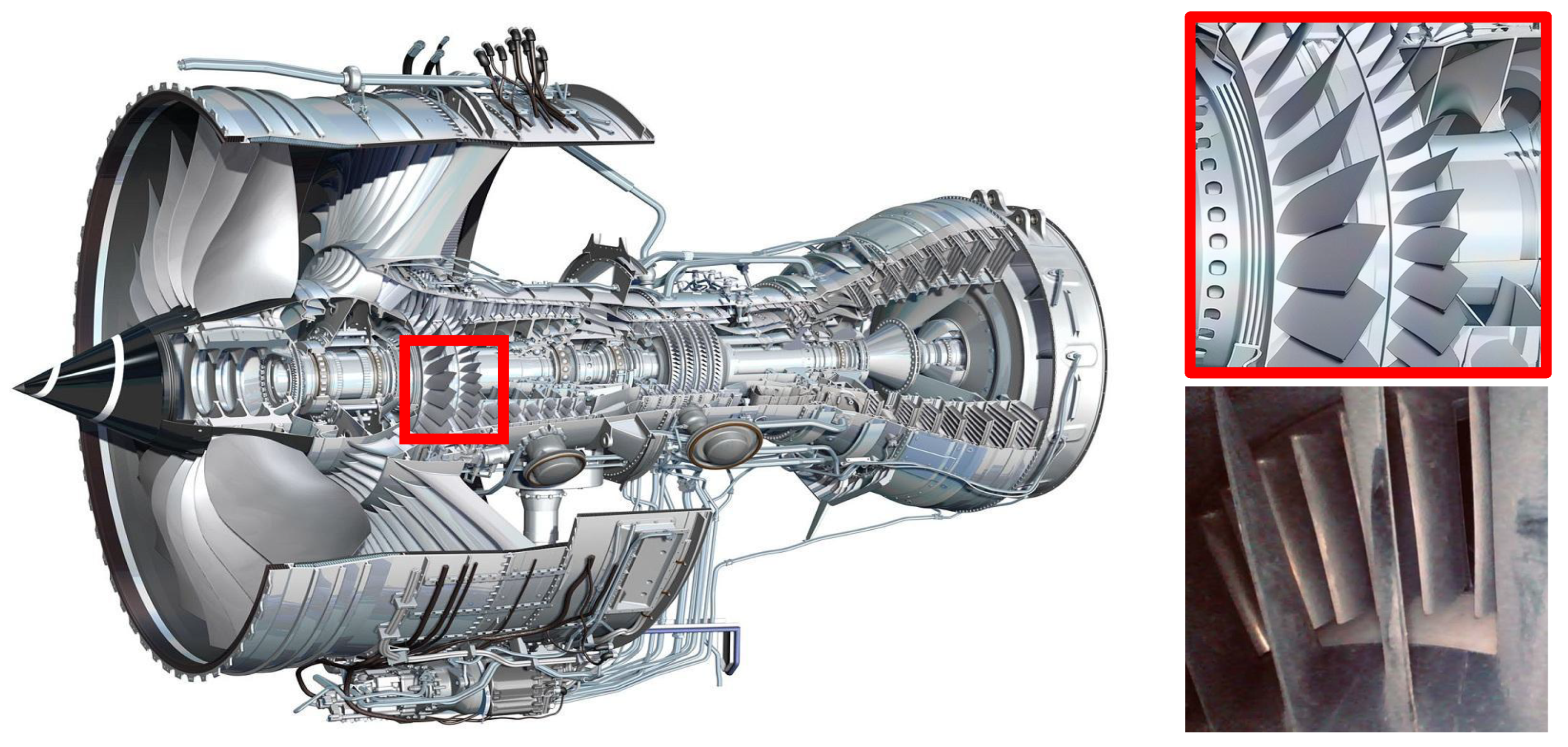
The images in the Turbo19 dataset used in this study were collected during real aero-engine inspection using an NTS500 industrial endoscope. This device can access complex internal regions of the aero-engine and acquire close-range images of key components, such as the high-pressure multi-stage compressor, thereby providing visual information for potential defect analysis.

Compared with common industrial surface images, aero-engine endoscopic images usually present more complex visual characteristics. On the one hand, metallic surfaces often contain complex textures, strong reflections, and illumination variations, which can introduce significant background interference. On the other hand, defect targets are usually small, slender, and ambiguous in boundary, and they often show low contrast against the surrounding background. These factors jointly increase the difficulty of precise defect segmentation and make this task more challenging in practical applications. Figure 1 illustrates the aero-engine endoscopic inspection process. Through this inspection system, complex internal regions of the engine can be observed in a non-destructive manner, providing image support for subsequent defect recognition and segmentation.

3.2. Turbo19 Dataset

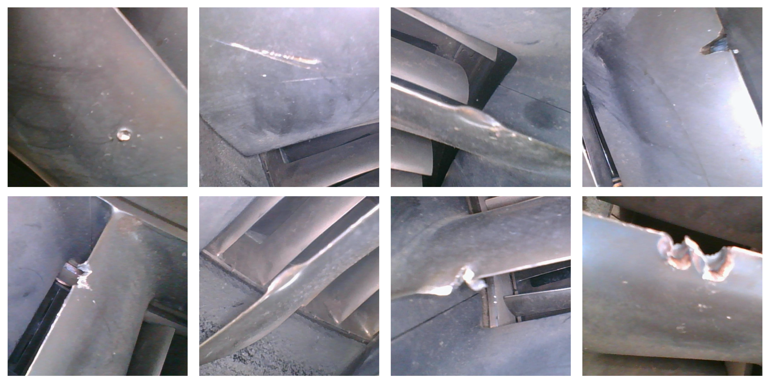
The Turbo19 dataset was carefully curated for our evaluation. It contains 5896 defect samples collected from aero-engines. All samples were collected during detailed inspections of the high-pressure multi-rotor compressor inside aero-engines (see Figure 2). The Turbo19 dataset was annotated in a pixel-wise manner. First, each image was manually labeled by two annotators with research experience in industrial image analysis. The annotations focused on defect contours and fine structural details. After the initial labeling stage, all samples were cross-checked, and inconsistent cases were reviewed jointly. A senior researcher with domain knowledge in aero-engine inspection performed the final quality control and resolved ambiguous cases. Images in the Free category were additionally verified to contain no visible defects under the adopted inspection criterion. The dataset includes the following defect categories:

• Curl: This defect is characterized by distorted contours. It is usually caused by aerodynamic forces during high-speed rotation or by material brittleness.
• Dent: This defect appears as a surface pit and is usually caused by foreign objects, such as small stones, during engine operation.
• Scratch: This defect is characterized by linear marks. It is typically produced by contact with abrasive materials during engine operation.
• Tearing: This defect appears as a torn surface on the material. It is usually caused by local stress concentration or external impact.
• Free: This category contains images without visible defects and provides a reference baseline for comparison in this study.

3.3. NEU-Seg Dataset

To further evaluate the segmentation capability of the proposed method under different industrial surface defect scenarios, experiments were also conducted on the NEU-Seg dataset. NEU-Seg is a widely used public dataset for industrial surface defect segmentation, containing 1800 hot-rolled steel strip surface defect images with corresponding pixel-level segmentation annotations. The dataset covers six typical types of steel surface defects, including rolled-in scale (RS), patches (Pa), cracks (Cr), pitted surface (PS), inclusions (In), and scratches (Sc). The images in the dataset exhibit large variations in defect morphology, scale, texture complexity, and background interference, which effectively reflect the complexity of real industrial inspection environments. In our experimental setup, the dataset was divided into a training set and a testing set with a ratio of 70% and 30%, respectively. The preprocessing pipeline for all images was kept consistent with that used for the Turbo19 dataset (

Table 1. Detailed statistics of the Turbo19 dataset.

Categories	Images	Percentage	Training	Testing
Curl	853	14.47%	597	256
Dent	1428	24.22%	1000	428
Scratch	1086	18.42%	760	326
Tearing	576	9.77%	403	173
Free	1953	33.12%	1367	586
Total	5896	100%	4127	1769

) to ensure fairness and comparability of the experiments.

4. Proposed Method

This section presents the proposed spectrum-driven hierarchical learning network. First, the overall framework is introduced. Then, the dual-band spectral module, the detail-guided module, the region-aware modeling module, and the loss function are described in detail.

4.1. Overview

A spectrum-driven hierarchical learning network is proposed for aero-engine defect segmentation. The goal is to achieve precise localization and segmentation of small defects in complex industrial environments. The proposed framework fully exploits frequency-domain information and regional structural differences. In this way, differentiated modeling is performed for defect interior regions, boundary regions, and background areas.

As shown in Figure 3, the overall pipeline first performs frequency-domain analysis on the input image. The original image is transformed into two complementary branches: a high-frequency branch and a low-frequency branch. These branches are used to represent detail information and global structural information, respectively. Next, the high-frequency features are integrated into the skip connections of the network through a detail-guided mechanism. This process compensates for the loss of fine-grained information caused by repeated downsampling in the encoding stage. At the same time, the low-frequency features are used to drive the region-aware modeling module. In the decoding stage, region-sensitive dynamic convolution kernels are generated to adapt to structural differences among different regions. The overall framework balances segmentation accuracy and model stability, and provides an effective solution for defect detection in aero-engine endoscopic images.

4.2. Dual-Band Spectral Module

In aero-engine defect detection tasks, surface defects (such as cracks, scratches, and local structural abnormalities) usually contain stronger high-frequency spectral features. These defects often appear as high-frequency components in the frequency domain, while the background regions are mainly concentrated in the low-frequency part. To effectively distinguish defects from the background, a dual-band spectral module is proposed in this study. This module explicitly separates the frequency-domain information of the image into two complementary parts: high-frequency and low-frequency components. In this way, the defect regions and background regions can be modeled separately.

The image is transformed into different frequency bands through the discrete cosine transform (DCT), which allows the image to be represented efficiently in a compact form. To preserve local information in the transformed spectrum, the transform is not applied to the entire image directly. Instead, the image is first divided into blocks, and the spectral transform is then computed independently within each block. Given an input image $x_{\mathrm{Gray}}\in {\mathbb{R}}^{1\times H\times W}$, the image is first divided into non-overlapping blocks with a size of $8\times 8$ pixels. After that, the discrete cosine transform (DCT) is applied to each $8\times 8$ block to generate the corresponding spectrum. In the spectrum of each $8\times 8$ block, the 64 coefficients correspond to 64 specific frequency components. To facilitate the subsequent filtering process, it is necessary to separate the different frequency components and group the same frequency components within each block. Therefore, the spectrum is reshaped. Specifically, the corresponding elements at the same position across all blocks (i.e., the same frequency component) are extracted and aggregated into one channel. In this way, a new spectral map $x_{\mathrm{DCT}}\in {\mathbb{R}}^{64\times H\times W}$ is obtained, which has 64 times the number of channels of the original spectrum while maintaining the same spatial resolution.

Each channel contains a specific frequency component. Therefore, filtering can be performed by selecting appropriate channels, which makes it easy to separate the frequency components represented by this tensor. In the generated spectral image, each channel corresponds to an independent frequency component. Frequency decomposition can thus be achieved through channel filtering operations. The corresponding formulations are shown in Equations (1)–(3):

$$M_H+M_L=1,$$

(1)

$$S_H=M_H\odot x_{\mathrm{DCT}},$$

(2)

$$S_L=M_L\odot x_{\mathrm{DCT}}.$$

(3)

Here, ⊙ denotes the Hadamard product. $M_H$ and $M_L$ represent the high-frequency mask and the low-frequency mask, respectively. $S_H$ and $S_L$ denote the high-frequency spectral features and the low-frequency spectral features, respectively.

In this module, the high-frequency spectral features are used in the subsequent network processing to enhance the detailed characteristics of defects, especially for the prediction of boundaries and textures. In contrast, the low-frequency spectral features help the network maintain consistent modeling of background regions and suppress background interference. Through this frequency-domain decoupling strategy, the network can better handle different types of surface defects, thereby improving detection performance.

4.3. Detail-Guided Module

During the multiple downsampling operations in the encoding stage, the high-frequency details described above can be weakened or lost. As a result, the decoder may not sufficiently describe defect boundaries and small defects. To address this problem, a detail-guided module is designed to introduce high-frequency spectral information into the skip connections and perform adaptive detail compensation for spatial features.

The detail-guided module follows a frequency-domain guidance strategy. The high-frequency spectral features extracted by the dual-band spectral modeling module are used as conditional information to generate guidance parameters. These parameters are then applied to the spatial feature representations in the skip connections. In this way, the model can selectively enhance defect-related details while preserving the original feature structure, thereby improving the representation ability of the segmentation results in boundary regions and small defect areas.

Let $F_{\mathrm{skip}}\in {\mathbb{R}}^{C\times H\times W}$ denote the spatial-domain skip connection feature map from the encoder, whose resolution is consistent with that of the corresponding decoder layer. First, the high-frequency spectral features are mapped through a lightweight transformation to generate channel-level feature guidance parameters, as shown in Equations (4) and (5):

$$\gamma =g_{\gamma }\left(S_H\right),$$

(4)

$$\beta =g_{\beta }\left(S_H\right),$$

(5)

where $g_{\gamma }(·)$ and $g_{\beta }(·)$ denote parameter generation functions implemented by $1\times 1$ convolution or equivalent linear mappings, and $\gamma ,\beta \in {\mathbb{R}}^{C\times 1\times 1}$. To ensure training stability and emphasize detail compensation, a residual-guided formulation is adopted to recalibrate the skip connection features, as shown in Equation (6):

$$F_{\mathrm{out}}=F_{\mathrm{skip}}\odot (1+\gamma )+\beta ,$$

(6)

where ⊙ denotes the Hadamard product. This formulation preserves the original spatial feature representation while introducing adaptive adjustments guided by high-frequency spectral information. Consequently, the fine-grained defect details and boundary structures are effectively enhanced.

The detail-guided module is embedded in the skip connections between the encoder and the decoder. For each decoder block, the skip connection features at the corresponding scale are first processed by the detail-guided module to perform high-frequency-guided detail enhancement. The resulting feature Fout is then fused with the current decoder features and used as the input to that decoder block. In this way, high-frequency detail information can be progressively propagated during the decoding process and can cooperate with low-level semantic information, thereby improving the segmentation accuracy in defect boundary regions and small-scale structural areas.

By introducing a high-frequency-guided feature mechanism into the skip connections, the loss of detailed information caused by downsampling in the encoding stage can be effectively compensated. Compared with traditional attention mechanisms, this module does not rely on complex explicit weighting structures. Instead, adaptive recalibration of spatial features is achieved through a guidance strategy driven by frequency-domain priors. As a result, the model remains lightweight while its ability to model fine-grained structures and boundary information in industrial defect segmentation tasks is enhanced.

4.4. Region-Aware Modeling Module

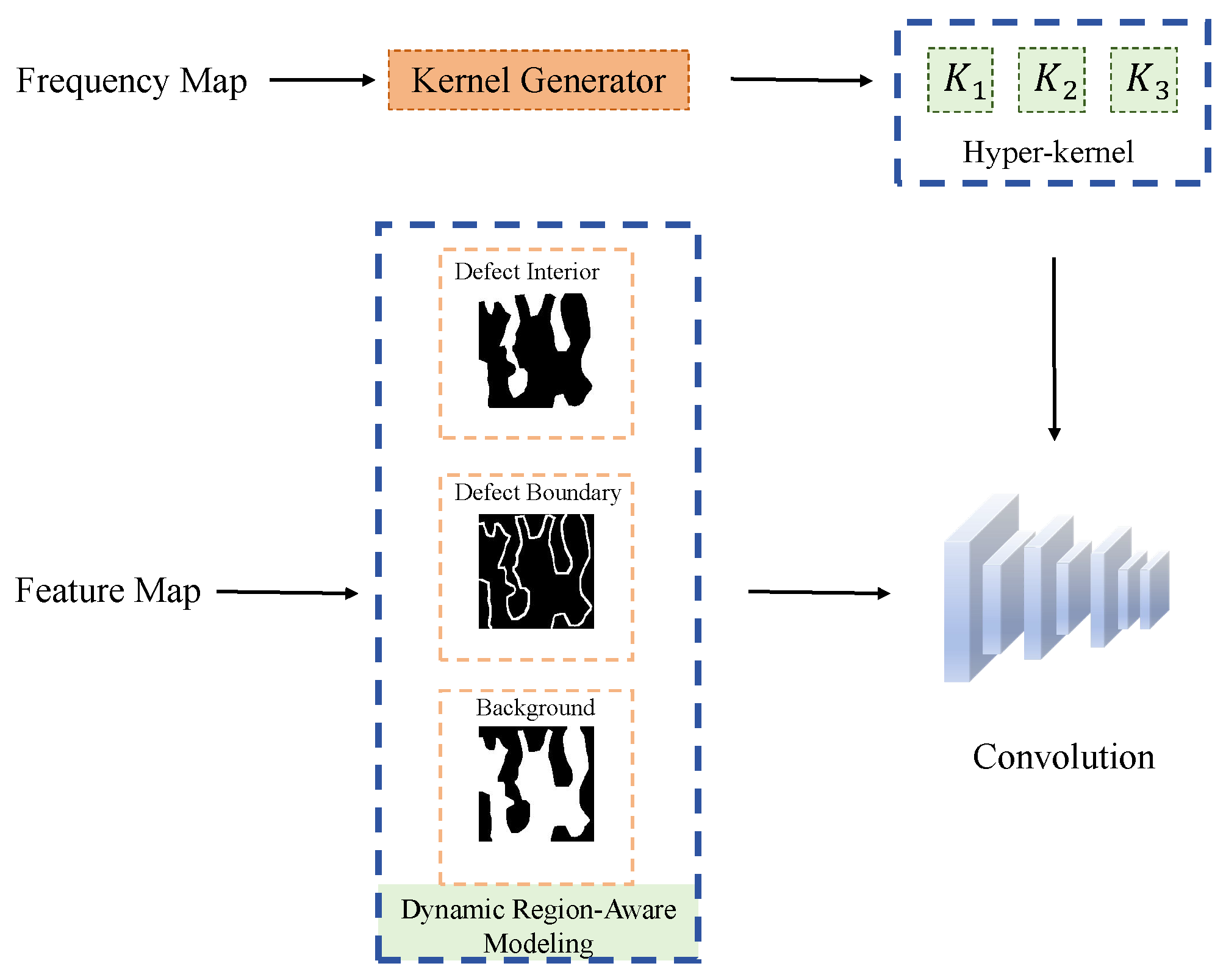
A low-frequency-driven region-aware modeling module is proposed to replace the standard weight-sharing convolution in the decoder. This design improves the model’s ability to adapt to appearance variations and operating condition changes on industrial surfaces. As shown in Figure 4, the module consists of two parts: dynamic region-aware modeling and low-frequency-driven hyper-kernel generation. First, under the guidance of hierarchical supervision, the dynamic region-aware modeling module learns adaptive region-level masks that represent the defect interior region, defect boundary region, and background region. These region-level masks are used to construct independent region-aware branches. In this way, the feature representations of different regions are modeled hierarchically. At each decoder stage, the structural characteristics of different regions are explicitly described, which enables region-aware feature modeling. Second, to better adapt to appearance variations caused by different industrial surface textures and imaging conditions, the low-frequency spectral features from the input image and the last encoder layer are utilized. A low-frequency-driven hyper-kernel generation module is designed to produce a set of region-sensitive hyper-kernels. These hyper-kernels are dynamically mapped at each decoder stage and are used to refine the hierarchical feature representations in the region-aware branches. As a result, adaptive modeling of regional structural consistency and contextual relationships can be achieved.

4.4.1. Dynamic Region-Aware Modeling

To achieve region-level feature modeling, the dynamic region-aware modeling module uses region-level masks to divide the feature representation into three regions with different structural properties: the defect interior region, the defect boundary region, and the background region. According to the structural characteristics of these regions, region-sensitive hyper-convolution kernels are applied to model the features of each region separately. In this way, the structural differences among regions can be explicitly described during the decoding stage.

The input feature map of the dynamic region-aware modeling module is denoted as $F_i$. First, region-level masks $M_j(j=1,2,3)$ are generated from the feature map $F_i$. Then, $F_i$ is multiplied with $M_j$ to obtain three regions within $F_i$: the defect interior region, the defect boundary region, and the background region, which are denoted as $R_j(j=1,2,3)$. Finally, each $R_j$ is convolved with the region-sensitive hyper-kernel $H_j(j=1,2,3)$, which is generated by the low-frequency-driven hyper-kernel generation module, to produce the final output $F_o$. The formulations are shown in Equations (7)–(9):

$$\begin{array}{c}{M}_j=\mathrm{Softmax}\left(\mathrm{Conv}\left(F_i\right)\right),j=1,2,3,\end{array}$$

(7)

$$\begin{array}{c}{R}_j=F_i\odot M_j,j=1,2,3,\end{array}$$

(8)

$$\begin{array}{c}{F}_o=\mathrm{concat}\left(\mathrm{Conv}(R_1;H_1),\mathrm{Conv}(R_2;H_2),\mathrm{Conv}(R_3;H_3)\right).\end{array}$$

(9)

To supervise the above region prediction, region-level ground truth masks are further constructed from the original binary defect annotation G. First, distance transform maps of the defect region and the background region are computed, which are denoted as $D_{in}$ and $D_{out}$, respectively. Here, $D_{in}$ represents the distance from an interior defect pixel to the nearest boundary, while $D_{out}$ represents the distance from a background pixel to the defect boundary. Let

$$d_{\max }=\max \left(D_{in}\right).$$

(10)

The inner boundary region and the outer boundary region of the defect are defined by Equations (11) and (12), respectively:

$$M_{in}^b=\mathbb{I}(0<D_{in}\le \alpha d_{\max }),$$

(11)

$$M_{out}^b=\mathbb{I}(0<D_{out}\le \alpha d_{\max }),$$

(12)

where $\alpha$ denotes the boundary ratio coefficient and is used to control the width of the boundary region, and $\mathbb{I}(·)$ denotes the indicator function [38,39]. Furthermore, to preserve the continuity of the defect contour, a contour consistency term $M_{ct}$ is introduced. The final defect boundary region is defined by Equation (13):

$$M_{bd}^{gt}=M_{in}^b\cup M_{out}^b\cup M_{ct}.$$

(13)

On this basis, the defect interior region and the background region are defined by Equations (14) and (15), respectively:

$$M_{in}^{gt}=\mathbb{I}(D_{in}>0)-M_{in}^b,$$

(14)

$$M_{bg}^{gt}=\mathbb{I}(D_{out}>0)-M_{out}^b.$$

(15)

In this way, the region-level supervision labels consist of three parts, namely the defect boundary region, the defect interior region, and the background region. The three region masks are concatenated in order to match the network output, and they are jointly used for the computation of the region-level supervision loss. This design allows the boundary width to adapt to the target scale, thereby enabling more stable modeling of the structural differences among the defect interior, the boundary transition region, and the background region.

4.4.2. Low-Frequency-Driven Hyper-Kernel Generation

The spectrum-based hyper-kernel generator produces a set of hyper-kernels for all decoder layers. The input consists of the low-frequency components of the image and the output from the final stage of the encoder. A linear projection obtained from the debiased frequency decomposition of the low-frequency features is treated as the query (Q), which helps reduce the influence of sample divergence. The number of queries is set to be the same as the number of hierarchical regions. In contrast, the key (K) and value (V) in the Transformer are generated from the low-level feature map $F_B$ in the encoder. This feature map is processed through positional encoding (PE) and projection to provide global spatial-domain information and spatial positional information. Since the hierarchical partition contains three semantic regions, namely the defect interior region, the defect boundary region, and the background region, three learnable region queries are constructed, one for each region. Each query corresponds to one region prototype and is used to generate the convolution kernel for that specific region. The output of the Transformer is then passed through a fully connected layer to adjust it to the required convolution kernel dimension, as shown in Equation (16):

$$H=\mathrm{FC}\left(\mathrm{Transformer}(Q,K,V)\right).$$

(16)

The Transformer outputs three region-specific latent embeddings, which are further projected into three region-sensitive hyper-kernels, denoted as $H_1$, $H_2$, and $H_3$. These three kernels correspond to the defect interior region, the defect boundary region, and the background region, respectively. Because the decoder contains multiple stages, the generated hyper-kernel tensor is further parsed according to both the decoder stage and the region category. Specifically, for the s-th decoder stage, one kernel triplet $\{H_1^{\left(s\right)},H_2^{\left(s\right)},H_3^{\left(s\right)}\}$ is assigned, where the three kernels are used for the defect interior region, the defect boundary region, and the background region, respectively. These kernels are then applied to convolve the corresponding region features $\{R_1^{\left(s\right)},R_2^{\left(s\right)},R_3^{\left(s\right)}\}$ in the dynamic region-aware modeling module. In this way, the kernel assignment is both region-specific and stage-dependent, enabling the decoder to perform adaptive convolutional modeling for different regions at different feature scales.

In this way, each decoder stage can use region-sensitive kernels that are better matched to the current feature scale and regional structure, thereby improving adaptive modeling of defect interiors, boundary transitions, and background regions.

Its key architectural innovation lies in a low-frequency-driven, hierarchically supervised, and stage-dependent hyper-kernel generation mechanism. The proposed module uses low-frequency spectral priors and encoder features to generate region-sensitive hyper-kernels, while explicitly learning and supervising defect interior, boundary, and background regions. The generated kernels are further assigned in a region-specific and decoder-stage-dependent manner, enabling frequency-guided hierarchical region-aware hyper-convolution.

4.5. Loss Function

The final loss function $L_{\mathrm{total}}$ consists of two parts: the segmentation supervision loss $L_{\mathrm{seg}}$ and the region-level mask loss $L_{\mathrm{mask}}$. These two losses jointly optimize the network from both the pixel level and the region level. The formulation is shown in Equation (17):

$$L_{\mathrm{total}}=L_{\mathrm{seg}}+\lambda L_{\mathrm{mask}}.$$

(17)

(a) Loss for segmentation results: The segmentation loss consists of the Focal loss and the intersection-over-union (IoU) loss. These two losses measure the pixel-level and region-level differences between the predicted segmentation result Y and the ground truth $GT$. They guide the network to learn a more accurate representation of the target regions. This loss improves the model’s ability to localize targets under complex backgrounds, enhances the representation of boundary details, and improves the overall structural consistency and stability of the segmentation results. The segmentation loss is defined as follows (Equation (18)):

$$L_{\mathrm{seg}}=L_{\mathrm{Focal}}(Y,GT)+L_{\mathrm{IoU}}(Y,GT).$$

(18)

(b) Loss for region-level masks: The region-level mask loss is defined as the mean squared error (MSE) loss. It is used to constrain the consistency between the predicted region masks and the ground truth region masks in terms of their continuous distributions. This loss guides the network to learn the spatial structural relationships among the defect interior region, the boundary transition region, and the background region, thereby improving the representation consistency within each region. The loss function is defined as follows (Equation (19)):

$$L_{\mathrm{mask}}=L_{\mathrm{MSE}}({\mathrm{Mask}}_{\mathrm{seg}},{\mathrm{Mask}}_{\mathrm{GT}}).$$

(19)

In summary, the combination of the segmentation supervision loss and the region-level mask loss forms a unified and effective optimization objective. Each component plays a specific role in guiding the model toward its corresponding learning goal. By properly setting the balancing parameter, the model can optimize both segmentation accuracy and region–structure representation during training.The overall procedure of the proposed method, namely the Spectrum-Driven Hierarchical Learning Network (Algorithm 1), is described as follows.

Algorithm 1: Spectrum-Driven Hierarchical Learning Network

Input: Input image x

Initialize: Generate spectral map $x_{\mathrm{DCT}}$ from x.

Step 1: Dual-Band Spectral Decomposition Apply DCT to the input image x; Decompose $x_{\mathrm{DCT}}$ into high-frequency features $S_H$ and low-frequency features $S_L$.

Step 2: Encoder Feature Extraction Feed the input image x into the encoder; Extract multi-scale encoder features.

Step 3: Detail-Guided Feature Enhancement Use high-frequency features $S_H$ to guide skip features $F_{\mathrm{skip}}$; Enhance fine defect details in the skip connections.

Step 4: Region-Aware Kernel Generation Use low-frequency features $S_L$ to generate region-sensitive kernels $\{H_1,H_2,H_3\}$; Assign the kernels to defect interior, defect boundary, and background regions.

Step 5: Hierarchical Region Modeling and Decoding Perform hierarchical modeling for defect interior, boundary, and background; Decode the features with the generated region-sensitive kernels; Obtain the segmentation result Y.

Output: Final segmentation map Y

5. Experiments and Results Analysis

This section introduces the experimental settings and evaluation metrics, and then reports comparison results, ablation studies, and further discussions to comprehensively validate the effectiveness of the proposed method.

5.1. Experimental Setup

5.1.1. Experimental Details

Implementation Details: All experiments were implemented in PyTorch 2.8.0 and conducted on an NVIDIA RTX 3080 Ti GPU. The images from the datasets were normalized and resized to $352\times 352$ pixels. A batch size of 8 was used to facilitate stable learning. An adaptive learning rate strategy was adopted. The initial learning rate was set to $1\times {10}^{-4}$, and it was reduced by a factor of 10 at the 50th epoch. The model was trained for 100 epochs. To ensure the reliability of the experimental results, each experiment was repeated five times with different random seeds, and the average performance of each method was reported.

5.1.2. Evaluation Metrics

To evaluate the performance of the model, five commonly used semantic segmentation metrics are adopted: mean Intersection over Union (mIoU), mean Pixel Accuracy (mPA), Precision, Recall, and F1-score. The definitions of these metrics are given as follows:

$$\mathrm{mIoU}={\displaystyle \frac{1}{C}}\sum _{c=1}^C{\displaystyle \frac{T{P}_c}{T{P}_c+F{P}_c+F{N}_c}},$$

(20)

where C denotes the number of categories, $T{P}_c$ represents the number of true positive pixels, $F{P}_c$ denotes the number of false positive pixels, and $F{N}_c$ denotes the number of false negative pixels.

$$\mathrm{mPA}={\displaystyle \frac{1}{C}}\sum _{c=1}^C{\displaystyle \frac{T{P}_c}{T{P}_c+F{N}_c}},$$

(21)

where $T{P}_c$ and $F{N}_c$ are defined as above.

$$\mathrm{Precision}={\displaystyle \frac{TP}{TP+FP}},$$

(22)

where TP denotes the number of true positive predictions and FP denotes the number of false positive predictions.

$$\mathrm{Recall}={\displaystyle \frac{TP}{TP+FN}},$$

(23)

where TP and FN are defined as above.

$$\mathrm{F}1={\displaystyle \frac{2\times \mathrm{Precision}\times \mathrm{Recall}}{\mathrm{Precision}+\mathrm{Recall}}},$$

(24)

where Precision and Recall are defined as above.

5.2. Comparison Methods and Fairness

The comparison experiments include seven segmentation methods, which are divided into three categories to enable a comprehensive evaluation. (1) Classical architectures: U-Net [40] and HarDNet-MSEG [41]. (2) CNN–Transformer architecture: Polyp-PVT [42]. (3) Boundary-aware architectures: PraNet [43], SANet [44], CFA-Net [45], and CCLDNet [46]. In the experiments, all comparison methods were implemented using their default or officially recommended parameter settings, without additional hyper-parameter tuning. Moreover, all methods were trained under the same basic experimental protocol, including image normalization and resizing to $352\times 352$ pixels, a batch size of 8, an initial learning rate of $1\times {10}^{-4}$, and 100 training epochs, in order to ensure a fair and unbiased comparison.

5.3. Results and Comparison

5.3.1. Qualitative Analysis

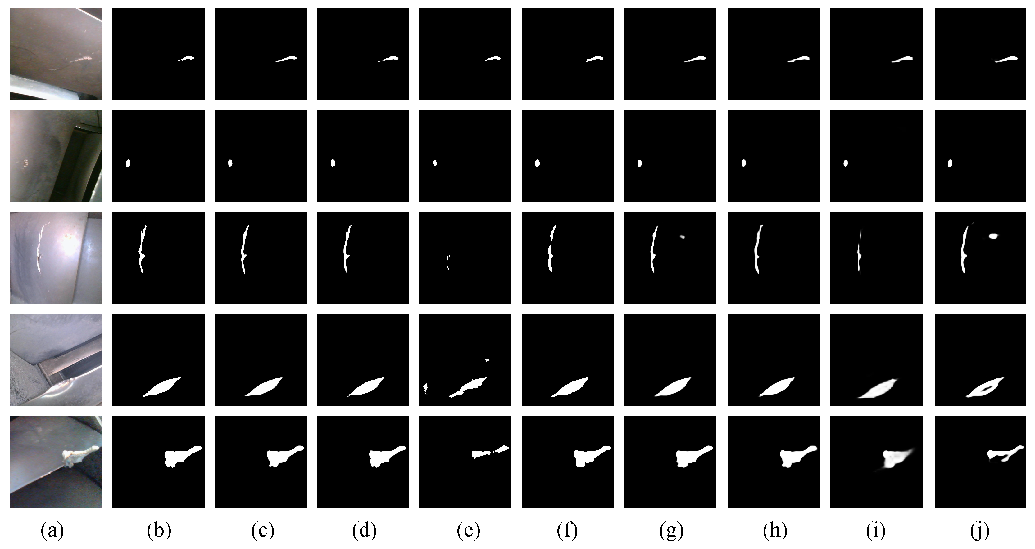
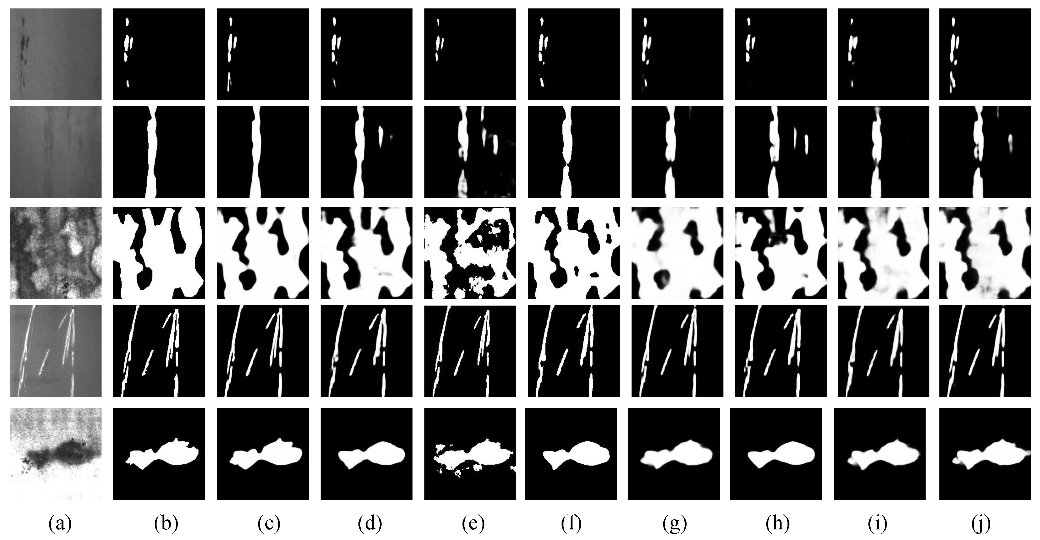
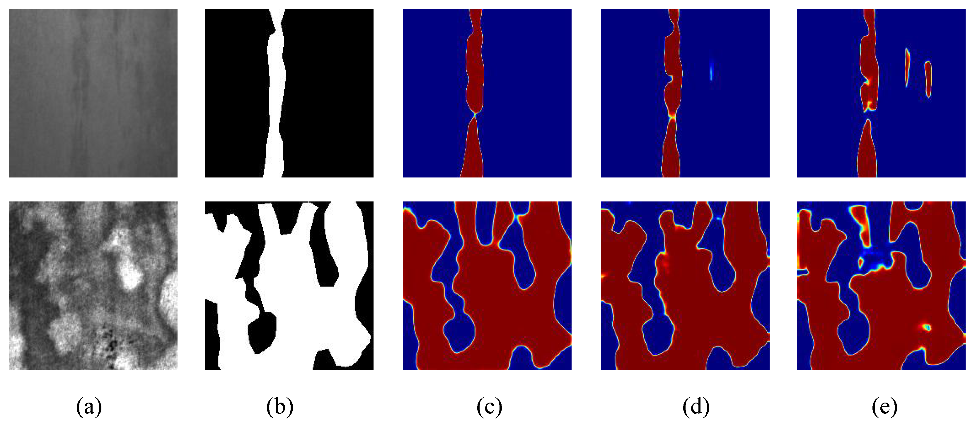
To comprehensively evaluate the effectiveness of the proposed method, both quantitative metrics and visualization results are analyzed. First, the visualization results on the Turbo19 and NEU-Seg datasets (see Figure 5 and Figure 6) show that different methods exhibit clear differences in defect boundary representation, detail recovery, and suppression of complex backgrounds. HarDNet-MSEG produces relatively stable segmentation results overall, but over-smoothing appears in slender cracks and boundary transition regions. U-Net lacks multi-scale and frequency-domain modeling ability, which leads to missed detections and false detections under complex metallic texture backgrounds. Polyp-PVT has strong global modeling capability, but its ability to recover local details is limited. CCLDNet performs well on large-scale defects, yet mis-segmentation occurs in complex background regions. PraNet shows strong boundary awareness, but the structural consistency within regions is insufficient. SANet significantly enhances boundary representation, but breaks often occur in very small and slender defects. CFA-Net shows weak robustness for low-contrast defects and presents obvious missed detections. In contrast, the proposed method produces segmentation results with clearer boundaries, more complete structures, and stronger background suppression on both datasets. These results demonstrate a stronger ability to represent small defects and a better adaptability to complex industrial scenarios. To provide a more intuitive comparison of local prediction details, additional colormap visualizations of representative challenging regions were added, as shown in Figure 7. These results more clearly reveal the differences among methods in boundary localization, weak defect activation, and background suppression.

5.3.2. Quantitative Discussion

Table 2. Quantitative comparison with state-of-the-art methods on the Turbo19 dataset.

	Turbo19 Dataset
Method	mIoU	Std.	mPA	Std.	Precision	Std.	Recall	Std.	F1-Score	Std.
MSEG	74.65	0.004	81.61	0.001	84.41	0.014	85.58	0.006	84.13	0.004
U-Net	69.39	0.012	75.61	0.004	79.89	0.005	80.63	0.008	79.06	0.010
Polyp-PVT	75.52	0.006	83.78	0.002	84.07	0.010	88.24	0.008	86.10	0.004
CCLDNet	84.60	0.003	87.47	0.002	85.06	0.007	87.13	0.007	86.08	0.003
PraNet	75.55	0.009	82.95	0.006	87.34	0.001	84.10	0.012	86.72	0.006
SANet	75.21	0.004	84.29	0.004	84.89	0.003	86.83	0.008	85.85	0.003
CFA-Net	70.63	0.004	76.50	0.003	73.49	0.005	78.46	0.004	75.82	0.014
Proposed	89.82	0.001	95.13	0.003	85.81	0.004	90.47	0.005	88.08	0.001

and

Table 3. Quantitative comparison with state-of-the-art methods on the NEU-Seg dataset.

	NEU-Seg Dataset
Method	mIoU	Std.	mPA	Std.	Precision	Std.	Recall	Std.	F1-Score	Std.
MSEG	78.39	0.001	86.61	0.001	87.75	0.004	87.63	0.005	87.06	0.001
U-Net	69.60	0.015	74.63	0.012	81.75	0.004	83.86	0.001	80.20	0.011
Polyp-PVT	80.25	0.007	85.36	0.007	87.77	0.006	90.76	0.010	89.23	0.002
CCLDNet	87.02	0.001	92.06	0.004	87.31	0.003	88.57	0.003	88.84	0.001
PraNet	82.55	0.007	93.52	0.014	90.50	0.008	90.38	0.002	90.44	0.004
SANet	82.22	0.012	92.44	0.008	90.22	0.007	89.26	0.009	90.24	0.005
CFA-Net	77.61	0.006	83.47	0.001	83.89	0.007	91.16	0.005	86.71	0.004
Proposed	91.44	0.001	96.88	0.003	91.77	0.002	92.93	0.006	92.34	0.001

report the quantitative results of the experiments, including the mean and variance of five evaluation metrics over five independent trials. It can be observed that the proposed method achieves the best mean performance across all metrics. For example, on the Turbo19 dataset, the proposed method improves the mIoU by 5.22% compared with the second-best method and achieves a 3.84% higher mPA score. On the NEU-Seg dataset, the proposed method improves the mIoU by 4.42% compared with the second-best method and obtains a 4.44% higher mPA score. In addition, the variance of each metric remains within an acceptable range, indicating stable model performance. These results support the effectiveness and stability of the proposed method in defect prediction. Moreover, the quantitative evidence is consistent with the qualitative observations and further confirms the effectiveness of the proposed method for aero-engine defect detection tasks.

5.4. Ablation Study

To verify the effectiveness of the dual-band spectral module (Module 1), detail-guided module (Module 2), and region-aware modeling module (Module 3), as well as the relationships among them, specific components were systematically removed from the proposed method. Four ablation variants were constructed, denoted as Variant 1, Variant 2, Variant 3, and Variant 4, as described below.

• Variant 1: Obtained by removing only the dual-band spectral module from the proposed method.
• Variant 2: Obtained by removing only the detail-guided module from the proposed method.
• Variant 3: Obtained by removing both the dual-band spectral module and the detail-guided module from the proposed method.
• Variant 4: Obtained by removing only the region-aware modeling module from the proposed method.

To ensure fairness in the experiments, all ablation variants were tested under the same experimental settings as the proposed method. The evaluations were conducted on both the Turbo19 dataset and the NEU-Seg Dataset.

In

Table 4. Ablation analysis on the Turbo19 dataset.

	Variant 1	Variant 2	Variant 3	Variant 4	Proposed
Module 1	×	✓	×	✓	✓
Module 2	✓	×	×	✓	✓
Module 3	✓	✓	✓	×	✓
mIoU	83.99	84.20	83.58	82.64	89.82
mPA	85.99	86.27	85.54	84.60	95.13

and

Table 5. Ablation analysis on the NEU-Seg dataset.

	Variant 1	Variant 2	Variant 3	Variant 4	Proposed
Module 1	×	✓	×	✓	✓
Module 2	✓	×	×	✓	✓
Module 3	✓	✓	✓	×	✓
mIoU	86.22	85.07	84.16	83.52	91.44
mPA	88.74	87.44	86.64	85.09	96.88

, the dual-band spectral module, the detail-guided module, and the region-aware modeling module are removed separately to evaluate the contribution of each component to the overall performance. On the Turbo19 dataset, when the dual-band spectral module is removed (Variant 1), the mIoU decreases from 89.82% to 83.99%, indicating that the frequency-domain decoupling of high-frequency and low-frequency information plays a key role in improving segmentation accuracy. When the detail-guided module is removed (Variant 2), the mIoU drops to 84.20%, demonstrating that the high-frequency detail compensation mechanism is essential for recovering boundary information lost during the downsampling process. When both the dual-band spectral module and the detail-guided module are removed (Variant 3), the performance further decreases to 83.58%, suggesting that frequency-domain modeling and detail guidance provide complementary benefits. When the region-aware modeling module is removed (Variant 4), the mIoU decreases to 82.64%, which represents the largest performance degradation. This result indicates that hierarchical region modeling is crucial for suppressing complex backgrounds and preserving structural consistency. A similar trend can be observed on the NEU-Seg dataset. The complete model achieves an mIoU of 91.44%, which is significantly higher than all ablation variants. These results verify the effectiveness of the three proposed modules under different industrial defect scenarios. Overall, the ablation study demonstrates that the dual-band spectral modeling improves the discriminative capability of feature representations, the detail-guided mechanism enhances boundary recovery, and the region-aware modeling module further strengthens regional structural consistency and background suppression. The collaborative integration of these three modules enables the proposed framework to achieve stable performance and significantly improved segmentation accuracy.

This is mainly because the designed modules play complementary and balanced roles at different feature levels. At the same time, all experimental results are reported as the average of three independent runs, and the performance variation is kept within a small range, which further demonstrates the stability of the model.

5.5. Further Discussion

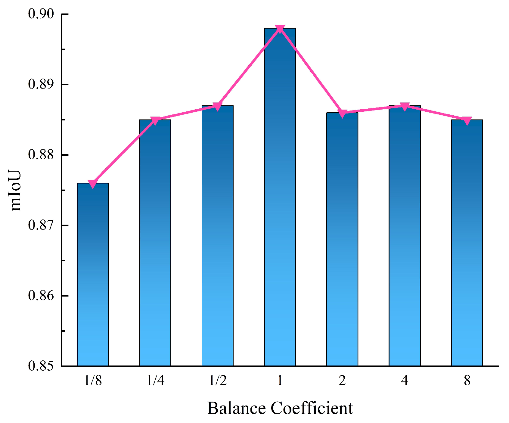
Balance Coefficient: Since $\lambda$ is a method-specific balancing coefficient in the proposed model, its effect was analyzed separately in this section rather than through additional tuning of the comparison methods. To further analyze the influence of the balance coefficient between the segmentation supervision loss and the region-level mask loss, the weighting parameter $\lambda$ was systematically investigated. Specifically, $\lambda$ was varied from $1/8$ to 8 with a scaling factor of 2 to evaluate the effect of different weighting strategies on model performance. To better understand the influence of the balance coefficient, the variations of $L_{\mathrm{seg}}$ and $L_{\mathrm{mask}}$ during training were visualized. As shown in Figure 8, when $\lambda$ changes within a relatively wide range, the fluctuations of key evaluation metrics, including mIoU and mPA, remain small and the overall performance stays stable.

This phenomenon indicates that the two loss terms maintain a cooperative relationship during optimization. The segmentation loss mainly constrains pixel-level prediction accuracy and ensures accurate localization of defect regions. In contrast, the region-level mask loss focuses on modeling the spatial relationships among the defect interior, boundary, and background, thereby improving the structural consistency of the segmentation results. When $\lambda$ is too small, the structural constraint provided by the region-level mask loss becomes weaker, which may lead to slightly coarse predictions in boundary transition regions. Conversely, when $\lambda$ is too large, the model emphasizes regional consistency more strongly, which may cause slight over-smoothing of fine-grained boundaries. Nevertheless, the overall performance variation remains limited, demonstrating that the proposed network is robust to changes in loss weights. This result further confirms that the region-aware modeling objective and the segmentation supervision objective are complementary rather than conflicting, ensuring stable training and reliable segmentation performance.

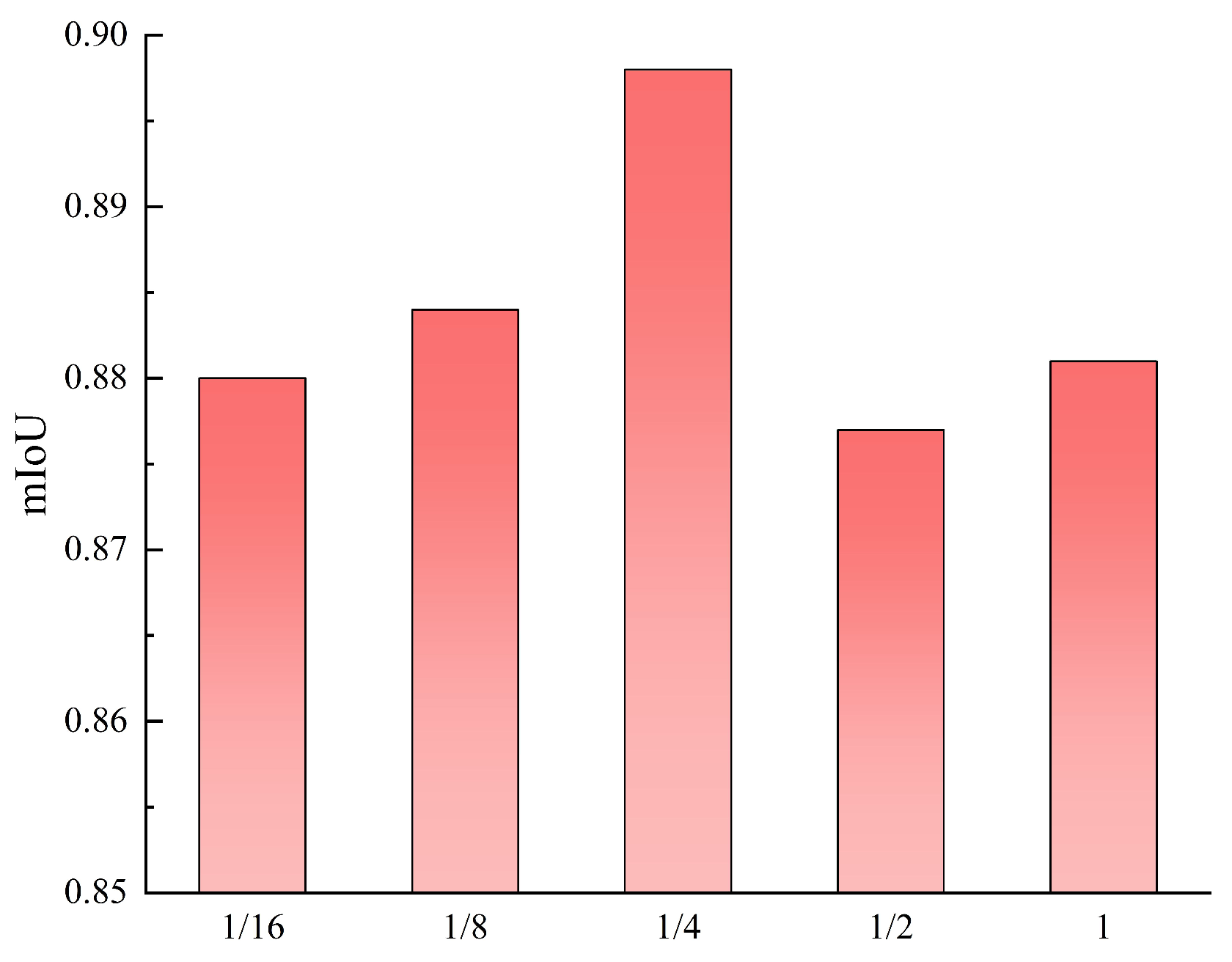
Boundary Region Size: To analyze the influence of the boundary region proportion in the region-level masks on model performance, a group of experiments was conducted by varying the boundary width while keeping all other training parameters unchanged. The boundary ratios were set to 1/16, 1/8, 1/4, 1/2, and 1, respectively. As shown in Figure 9, the model performance shows a clear trend as the boundary ratio changes. When the ratio increases from 1/16 to 1/4, the mIoU gradually improves and reaches its highest value at 1/4. However, when the ratio is further increased to 1/2 and 1, the performance begins to decline. When the ratio is small, the boundary region occupies only a limited proportion of the overall region partition. As a result, its contribution to the training objective is relatively small, and the boundary constraint may not be sufficiently exploited. As the ratio increases moderately, the boundary region participates more actively in the optimization process, which helps improve the overall segmentation accuracy. However, when the ratio becomes too large, the boundary region occupies a greater number of pixels. This may reduce the discriminative space between the defect interior region and the background region, weakening the differences among regions and consequently affecting the overall model performance.

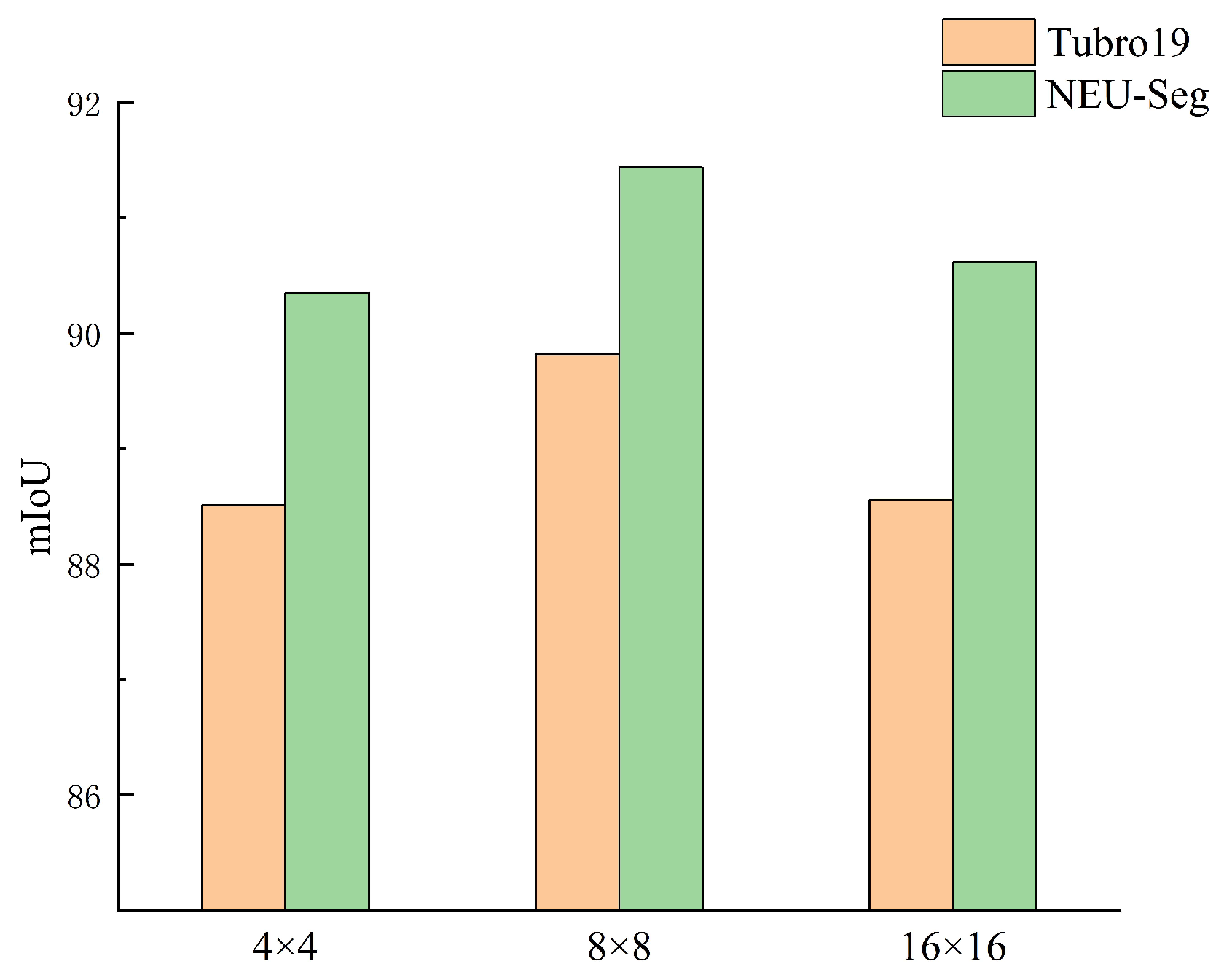
DCT Block Size Analysis: To evaluate the influence of the DCT block size on segmentation performance, three settings, including 4 × 4, 8 × 8, and 16 × 16, were further compared. As illustrated in Figure 10, the 8 × 8 configuration achieved the best overall performance on both the Turbo19 and NEU-Seg datasets. Specifically, the mIoU reached 89.82% on Turbo19 and 91.44% on NEU-Seg, which was higher than those obtained with 4 × 4 and 16 × 16 blocks. This result suggests that 8 × 8 provides a more suitable trade-off between local spatial sensitivity and frequency representation capability. A smaller block size such as 4 × 4 preserves local information, but its frequency resolution is limited. In contrast, a larger block size such as 16 × 16 provides coarser local spectral modeling, which may weaken the representation of small defects under complex backgrounds. Therefore, the 8 × 8 block size was selected in our method.

6. Conclusions

In this study, a spectrum-driven hierarchical learning framework is proposed. The method explicitly introduces frequency-domain information and combines it with regional structural modeling to achieve stable representation and precise localization of small defects. In the proposed framework, a dual-band spectral module is first designed. The discrete cosine transform is used to decompose the image spectrum, and the image features are explicitly separated into high-frequency detail information and low-frequency structural information. In this way, physically meaningful frequency-domain priors are provided for the network. Next, the high-frequency spectral information is introduced into the skip connections through a detail-guided module. This module adaptively compensates for the fine-grained information lost during downsampling in the encoding stage, thereby enhancing the representation of defect boundaries and small structural details. Furthermore, a region-aware modeling module is proposed. Low-frequency features are used to drive region-level structural modeling, and a dynamic hyper-kernel generation mechanism is employed to implement region-sensitive convolution. This design enables the network to perform differentiated feature modeling for the defect interior region, boundary region, and background region. Experiments on two datasets demonstrate the effectiveness of the proposed method and suggest its potential applicability to other industrial inspection tasks beyond aero-engine inspection. It is worth noting that the performance drops caused by removing each individual module are relatively similar.

References

- Qi, H.; Cheng, L.; Kong, X.; Zhang, J.; Gu, J. WDLS: Deep level set learning for weakly supervised aeroengine defect segmentation. IEEE Trans. Ind. Inform. 2023, 20, 303–313. [Google Scholar] [CrossRef]
- Huang, J.; Wu, Y.; Zhou, X.; Lin, J.; Chen, Z.; Zhang, G.; Xia, L.; Zhang, J. Multi-scale adaptive prototype transformer network for few-shot strip steel surface defect segmentation. IEEE Trans. Instrum. Meas. 2025, 74, 5016514. [Google Scholar]
- Shan, Z.; Hu, H.; Zhu, C.; Du, S.; Jing, H.; Wang, H. RSM-YOLOv11: Lightweight steel surface defect segmentation algorithm based on YOLOv11 improvement. IEEE Access 2025, 13, 111681–111698. [Google Scholar] [CrossRef]
- Wang, H.; Wang, K.-N.; Hua, J.; Tang, Y.; Chen, Y.; Zhou, G.-Q.; Li, S. Dynamic spectrum-driven hierarchical learning network for polyp segmentation. Med. Image Anal. 2025, 101, 103449. [Google Scholar] [CrossRef] [PubMed]
- Ameri, R.; Hsu, C.-C.; Band, S.S. A systematic review of deep learning approaches for surface defect detection in industrial applications. Eng. Appl. Artif. Intell. 2024, 130, 107717. [Google Scholar] [CrossRef]
- Mao, Y.; Chen, Z.; Liu, Y.; Dong, C.; Song, K. A survey on industrial image anomaly detection: Methods, benchmarks and rethinks. Measurement 2025, 256, 118377. [Google Scholar] [CrossRef]
- Wen, G.; Cheng, L.; Yuan, H.; Li, X. Surface defect detection based on adaptive multi-scale feature fusion. Sensors 2025, 25, 1720. [Google Scholar] [CrossRef]
- Xia, Y.; Lu, Y.; Jiang, X.; Xu, M. Enhanced multiscale attentional feature fusion model for defect detection on steel surfaces. Pattern Recognit. Lett. 2025, 188, 15–21. [Google Scholar] [CrossRef]
- Ma, Y.; Yin, J.; Huang, F.; Li, Q. Surface defect inspection of industrial products with object detection deep networks: A systematic review. Artif. Intell. Rev. 2024, 57, 333. [Google Scholar] [CrossRef]
- Dong, X.; Li, Y.; Fu, L.; Liu, J. Edge-aware interactive refinement network for strip steel surface defects detection. Meas. Sci. Technol. 2025, 36, 016222. [Google Scholar] [CrossRef]
- Wang, Y.; Zhu, Y.; Chen, X.; Yin, T.; Su, S. Steel Surface Defect Detection via the Multiscale Edge Enhancement Method. Comput. Mater. Contin. 2026, 86, 40. [Google Scholar] [CrossRef]
- Cheng, Y.; Cao, Y.; Yao, H.; Luo, W.; Jiang, C.; Zhang, H.; Shen, W. A comprehensive survey for real-world industrial surface defect detection: Challenges, approaches, and prospects. J. Manuf. Syst. 2026, 84, 152–172. [Google Scholar] [CrossRef]
- Kim, D.; Gerstberger, U.; Asli, M.; Höschler, K. U-Net driven semantic segmentation for detection and quantification of cracks on gas turbine blade tips. Results Eng. 2025, 29, 108864. [Google Scholar] [CrossRef]
- Zhou, Y.; Wu, H.; Wang, Y.; Liu, X.; Zhai, X.; Sun, K.; Zheng, Z.; Tian, C.; Zhao, H.; Jia, W.; et al. PIndNet: A pixel-wise industrial defect inspection network using multiple pyramid feature aggregation. Measurement 2025, 245, 116639. [Google Scholar] [CrossRef]
- Liu, Y.; Zhang, C.; Dong, X. A survey of real-time surface defect inspection methods based on deep learning. Artif. Intell. Rev. 2023, 56, 12131–12170. [Google Scholar] [CrossRef]
- Nahar, L.; Awrangjeb, M.; Islam, M.S. AI-enabled defect detection in industrial products: A comprehensive survey, key insights and future research challenges. Adv. Eng. Inform. 2026, 69, 104067. [Google Scholar] [CrossRef]
- He, Y.; Li, S.; Wen, X.; Xu, J. A survey on surface defect inspection based on generative models in manufacturing. Appl. Sci. 2024, 14, 6774. [Google Scholar] [CrossRef]
- Yang, Z.; Yu, H.; Zhang, J.; Tang, Q.; Mian, A. Deep learning based infrared small object segmentation: Challenges and future directions. Inf. Fusion 2025, 118, 103007. [Google Scholar] [CrossRef]
- Celik, M.; Inik, O. Review of deep learning-based segmentation methods: Popular approaches, literature gaps, and opportunities. Displays 2025, 91, 103225. [Google Scholar] [CrossRef]
- Montello, F.; Güldenring, R.; Scardapane, S.; Nalpantidis, L. A survey on dynamic neural networks: From computer vision to multi-modal sensor fusion. Image Vis. Comput. 2026, 105980. [Google Scholar] [CrossRef]
- Lee, D.H.; Park, H.Y.; Lee, J. A review on recent deep learning-based semantic segmentation for urban greenness measurement. Sensors 2024, 24, 2245. [Google Scholar] [CrossRef]
- Yang, L.; Fan, J.; Huo, B.; Li, E.; Liu, Y. A nondestructive automatic defect detection method with pixelwise segmentation. Knowl.-Based Syst. 2022, 242, 108338. [Google Scholar] [CrossRef]
- Tsai, D.-M.; Fan, S.-K.S.; Chou, Y.-H. Auto-annotated deep segmentation for surface defect detection. IEEE Trans. Instrum. Meas. 2021, 70, 5011410. [Google Scholar] [CrossRef]
- Xu, H.; Yan, Z.; Ji, B.; Huang, P.; Cheng, J.; Wu, X. Defect detection in welding radiographic images based on semantic segmentation methods. Measurement 2022, 188, 110569. [Google Scholar] [CrossRef]
- Yang, X.; Song, K.; Liu, S.; Sun, F.; Zheng, Y.; Li, J.; Yan, Y. An edge-guided defect segmentation network for in-service aerospace engine blades. Eng. Appl. Artif. Intell. 2025, 154, 110974. [Google Scholar] [CrossRef]
- Song, M.; Zhang, Y. Aviation-engine blade surface anomaly detection based on the deformable neural network. Signal Image Video Process. 2025, 19, 87. [Google Scholar] [CrossRef]
- Utomo, S.; Sulistyaningrum, D.R.; Setiyono, B.; Mubarok, M.K.N. Recurrent Residual U-Net for borescope crack segmentation in aero-engine. In International Conference on Informatics, Multimedia, Cyber and Information System (ICIMCIS); IEEE: New York, NY, USA, 2025; pp. 1323–1328. [Google Scholar]
- Liu, Y.; Liu, J.; Xu, Y.; Fu, Q.; Qian, J.; Wang, X. Aero-engine ablation defect detection with improved CLR-YOLOv11 algorithm. Sensors 2025, 25, 6574. [Google Scholar] [CrossRef]
- Wang, R.; Du, W.; Jiang, Q.; Cao, Z. Defect detection in impeller parts utilising local geometric feature analysis. Int. J. Prod. Res. 2025, 63, 6475–6492. [Google Scholar] [CrossRef]
- Yang, L.; Xu, S.; Fan, J.; Li, E.; Liu, Y. A pixel-level deep segmentation network for automatic defect detection. Expert Syst. Appl. 2023, 215, 119388. [Google Scholar] [CrossRef]
- Zuo, L.; Xiao, H.; Wen, L.; Gao, L. A pixel-level segmentation convolutional neural network based on global and local feature fusion for surface defect detection. IEEE Trans. Instrum. Meas. 2023, 72, 5029510. [Google Scholar] [CrossRef]
- Qi, H.; Kong, X.; Wang, Z.; Gu, J.; Cheng, L. AeroClick: An advanced single-click interactive framework for aeroengine defect segmentation. Expert Syst. Appl. 2024, 257, 125093. [Google Scholar] [CrossRef]
- Meng, D.; Wu, B.; Xu, J.; Zuo, H. Visual inspection of aircraft skin: Automated pixel-level defect detection by instance segmentation. Chin. J. Aeronaut. 2022, 35, 254–264. [Google Scholar] [CrossRef]
- Qi, H.; Kong, X.; Liu, Z.; Gu, J.; Cheng, L. SAIT: Harnessing sparse annotations and intrinsic tasks for semi-supervised aeroengine defect segmentation. IEEE Trans. Ind. Inform. 2024, 20, 10463–10472. [Google Scholar] [CrossRef]
- Zhang, Y.; Ge, W.; Liu, S.; Wang, J.; Hu, H.; Dong, J.; Zhang, T. An adaptive feature refinement network for pixel-level segmentation of surface defect. Meas. Sci. Technol. 2024, 36, 016197. [Google Scholar] [CrossRef]
- Ma, Y.; Liu, M.; Zhang, Y.; Wang, X.; Wang, Y. SPDP-Net: A semantic prior guided defect perception network for automated aero-engine blades surface visual inspection. IEEE Trans. Autom. Sci. Eng. 2024, 22, 2724–2733. [Google Scholar] [CrossRef]
- Sun, Y.; Liu, X.; Zhai, X.; Sun, K.; Zhao, M.; Chang, Y.; Zhang, Y. Automatic pixel-level detection of tire defects based on a lightweight Transformer architecture. Meas. Sci. Technol. 2023, 34, 085405. [Google Scholar] [CrossRef]
- Pham, H.C.; Ta, Q.-B.; Kim, J.-T.; Ho, D.-D.; Tran, X.-L.; Huynh, T.-C. Bolt-loosening monitoring framework using an image-based deep learning and graphical model. Sensors 2020, 20, 3382. [Google Scholar] [CrossRef]
- Kim, J.-T.; Ta, Q.-B.; Dang, N.-L.; Kim, Y.-C.; Kam, H.-D. Semantic crack-image identification framework for steel structures using atrous convolution-based Deeplabv3+ Network. Smart Struct. Syst. Int. J. 2022, 30, 17–34. [Google Scholar]
- Ronneberger, O.; Fischer, P.; Brox, T. U-Net: Convolutional networks for biomedical image segmentation. In International Conference on Medical Image Computing and Computer-Assisted Intervention; Springer: Cham, Switzerland, 2015; pp. 234–241. [Google Scholar]
- Huang, C.-H.; Wu, H.-Y.; Lin, Y.-L. HarDNet-MSEG: A simple encoder-decoder polyp segmentation neural network that achieves over 0.9 mean dice and 86 FPS. arXiv 2021, arXiv:2101.07172. [Google Scholar]
- Dong, B.; Wang, W.; Fan, D.-P.; Li, J.; Fu, H.; Shao, L. Polyp-PVT: Polyp segmentation with pyramid vision transformers. arXiv 2021, arXiv:2108.06932. [Google Scholar] [CrossRef]
- Fan, D.-P.; Ji, G.-P.; Zhou, T.; Chen, G.; Fu, H.; Shen, J.; Shao, L. PraNet: Parallel reverse attention network for polyp segmentation. In International Conference on Medical Image Computing and Computer-Assisted Intervention; Springer: Cham, Switzerland, 2020; pp. 263–273. [Google Scholar]
- Wei, J.; Hu, Y.; Zhang, R.; Li, Z.; Zhou, S.K.; Cui, S. Shallow attention network for polyp segmentation. In International Conference on Medical Image Computing and Computer-Assisted Intervention; Springer: Cham, Switzerland, 2021; pp. 699–708. [Google Scholar]
- Zhou, T.; Zhou, Y.; He, K.; Gong, C.; Yang, J.; Fu, H.; Shen, D. Cross-level feature aggregation network for polyp segmentation. Pattern Recognit. 2023, 140, 109555. [Google Scholar] [CrossRef]
- Yang, H.; Chen, Q.; Fu, K.; Zhu, L.; Jin, L.; Qiu, B.; Ren, Q.; Du, H.; Lu, Y. Boosting medical image segmentation via conditional-synergistic convolution and lesion decoupling. Comput. Med. Imaging Graph. 2022, 101, 102110. [Google Scholar] [CrossRef] [PubMed]
Figure 1.
Schematic illustration of aero-engine endoscopic inspection.
Figure 2.
Visual examples from the Turbo19 dataset.
Figure 3.
Overview of the proposed framework. The framework consists of three modules: a Dual-Band Spectral Module, a Detail-Guided Module, and a Region-Aware Modeling Module. The spectral module separates the input into high- and low-frequency features. High-frequency features guide skip connections to recover fine details, while low-frequency features generate region-sensitive hyper-kernels for hierarchical modeling of defect interior, boundary, and background regions.
Figure 4.
Illustration of the region-aware modeling module.
Figure 5.
Prediction results on the Turbo19 dataset. (a) Image. (b) Ground truth. (c) Ours. (d) MSEG. (e) U-Net. (f) Polyp-PVT. (g) CCLDNet. (h) PraNet. (i) SANet. (j) CFA-Net.
Figure 6.
Prediction results on the NEU-Seg Dataset. (a) Image. (b) Ground truth. (c) Ours. (d) MSEG. (e) U-Net. (f) Polyp-PVT. (g) CCLDNet. (h) PraNet. (i) SANet. (j) CFA-Net.
Figure 7.
Colormap visualizations on the NEU-Seg dataset. (a) Zoomed input image. (b) Ground truth. (c) Ours. (d) MSEG. (e) PraNet. The colormap responses provide a more intuitive basis for comparing boundary localization, defect activation, and suppression of background interference.
Figure 8.
Impact of the loss function balancing coefficient.
Figure 9.
Impact of the boundary region proportion.
Figure 10.
Effect of DCT block size.