Article

Numerical Error Analysis of the Poisson Equation Under RHS Inaccuracies in Particle-in-Cell Simulations

1
Department of Computer and Electric Engineering, Hunan University of Arts and Science, 3150 Dongting Avenue, Changde 415000, China
2
Hunan Provincial Key Laboratory for Control Technology of Distributed Electric Propulsion Aircraft, Changde 415000, China
3
School of Aerospace Engineering, Beihang University, 37 Xueyuan Road, Haidian District, Beijing 100191, China
*
Author to whom correspondence should be addressed.
Computation 2026, 14(1), 13; https://doi.org/10.3390/computation14010013
Submission received: 1 December 2025 / Revised: 30 December 2025 / Accepted: 4 January 2026 / Published: 7 January 2026
(This article belongs to the Section Computational Engineering)

Abstract

Particle-in-Cell (PIC) simulations require accurate solutions of the electrostatic Poisson equation, yet accuracy often degrades near irregular Dirichlet boundaries on Cartesian meshes. While prior work has focused on left-hand-side (LHS) discretization errors, the impact of right-hand-side (RHS) inaccuracies arising from charge deposition near boundaries remains largely unexplored. This study analyzes numerical errors induced by underestimated RHS values at near-boundary nodes when using embedded finite difference schemes with linear and quadratic boundary treatments. Analytical results in one dimension and truncation error analyses in two dimensions show that RHS inaccuracies affect the two schemes in fundamentally different ways: They reduce boundary-induced errors in the linear scheme but introduce zeroth-order truncation errors in the quadratic scheme, leading to larger global errors. Numerical experiments in one, two, and three dimensions confirm these predictions. In two-dimensional tests, RHS inaccuracies reduce the L error of the linear scheme by a factor of 2–3, while increasing the quadratic-scheme error by several times, and in some cases by nearly an order of magnitude, with both schemes retaining second-order global convergence. A simple δ ¯ -based RHS calibration is proposed and shown to effectively restore the accuracy of the quadratic scheme.

Graphical Abstract

1. Introduction

Particle-in-Cell [1] (PIC) simulation has become an indispensable tool in studying plasma physics, where a core computational task is solving the electrostatic Poisson equation on a mesh. Most modern PIC codes [2,3,4,5,6] for simulating plasma flows adopt Cartesian meshes, owing to advantages such as straightforward implementation, efficient parallelization, and favorable computational performance. While Cartesian PIC codes can, in principle, accommodate arbitrarily shaped boundaries, solution accuracy often degrades in the presence of irregular Dirichlet boundaries. This degradation arises because mesh nodes rarely align perfectly with the boundary surfaces. For geometries with high symmetry—such as spherical or cylindrical shapes—these challenges can be alleviated by developing customized PIC codes using spherical [7,8,9] or cylindrical meshes [10,11,12]. However, such specialized codes are only applicable to a limited class of problems and typically require substantial development effort. Other approaches, such as finite-volume-based methods [13] or finite-element methods [14,15,16], fundamentally alter the structure of standard PIC codes, introducing additional complexity and reduced computational efficiency.
There were many existing techniques for improving the accuracy of solutions to the Poisson equation on irregular domains on Cartesian meshes, each providing a unique way to reduce truncation errors at near-boundary nodes, defined as nodes less than one grid spacing away from boundary interfaces in any coordinate direction. For example, Mayo’s method [17,18,19] that employ the integral formations for the near-boundary nodes. While this method allows the use of fast Poisson solvers [20], the procedures require using numerical quadrature to evaluate the integrals followed by spline interpolations. In solving more general elliptic equations, the immersed interface method (IIM) proposed by LeVeque and Li [21,22] introduces an innovative six-point stencil for the near-boundary nodes, which necessitates determining appropriate coefficients for the stencil points by solving local linear systems. Both approaches have been proved to produce second-order accuracy [23]. The embedded boundary finite volume methods [24,25] are viable alternatives, with the scheme of Devendran et al. [25] achieving fourth-order accuracy.
Among second-order accurate methods, the embedded boundary finite difference method offers an attractive alternative [26,27]. This method embeds irregular Dirichlet boundaries within a rectangular (or cuboidal in 3D) computational domain and modifies the Poisson equation’s discretization near the boundary using either the linear [28] or the quadratic interpolation schemes [29,30]. For interior grid nodes located at least one grid spacing away from the Dirichlet boundaries along any axial direction, the standard five-point stencil, known to yield second-order truncation error, is retained. The resulting discretization yields a linear system that can be solved numerically.
Extensive prior work has investigated the error behavior of the embedded boundary finite difference method. It is widely recognized that both the linear and quadratic schemes improve the solution accuracy. In particular, the linear scheme was proved to give second-order accuracy [28], while the quadratic attains third-order accuracy at the boundaries and maintains second-order accuracy in the interior [30,31,32]. These two schemes have been successfully applied in various computational applications, including crystal growth [33], fluid dynamics [34], tumor modeling [35], etc. Recently, the use of such schemes has also seen increases in plasma simulations [36,37]. The linear scheme, in particular, has been considered favorable [28] for its simplicity and the symmetric linear systems it produces, which enables using efficient sparse matrix storage and matrix-vector algorithms, as well as iterative solvers such as the Preconditioned Conjugate Gradient (PCG) method. However, Jomaa and Macaskill’s error analysis [26] challenged the preference for the linear scheme. In one-dimensional problems, they provided explicit numerical error expressions. Upon evaluating these expressions, we found that the linear scheme, although exhibiting second-order accuracy, has much larger error coefficients than the quadratic counterpart. For two-dimensional problems, they numerically verified that their 1D error analysis holds at non-corner grid points.
While the majority of existing studies focus on discretization errors arising from the numerical treatment of the left-hand side (LHS) of the Poisson equation, comparatively little attention has been paid to inaccuracies originating from the right-hand side (RHS). LHS errors are intrinsic to the discretization of the differential operator and have been extensively analyzed. RHS errors, in contrast, arise from inaccuracies in the data rather than from the Poisson solver itself, for example due to measurement errors in fluid dynamics [38,39] or particle-to-grid weighting procedures [40] in PIC applications. In practice, both sources of error are important; however, once a sufficiently accurate LHS discretization is used, RHS inaccuracies become the limiting factor for the overall solution accuracy. We note that alternative solution paradigms for Poisson-type equations, including semi-analytical methods [41], physics-informed neural networks [42], and heuristic algorithms [43], have also been explored in the literature; however, these approaches generally do not examine RHS inaccuracies near Dirichlet boundaries in classical grid-based solvers.
Several studies in the literature have examined the Poisson equation with varied RHS values. Pan et al. [38,39] investigated the pressure Poisson equation in the context of particle image velocimetry (PIV) for fluid dynamics. In their formulation, the RHS depends on experimentally measured velocity-field data, which inevitably contain systematic errors across the domain. They derived error bounds for the reconstructed pressure field and numerically validated these bounds under the assumption of constant perturbations in the RHS at both interior and boundary points. However, their analysis did not account for irregular Dirichlet boundary effects, nor did it consider numerical errors arising from solving the Poisson equation. Marques et al. [44] developed the Correction Function Method (CFM) to handle interface jump conditions for constant-coefficient Poisson equations. As a finite difference approach, this method estimates ghost-node values that can be incorporated into the RHS, thereby enabling the use of standard solvers. Although the method modifies the RHS, its primary purpose is to improve the discretization of the LHS; hence, it does not address inaccuracies in the RHS itself.
A critical gap in the literature concerns the effect of RHS inaccuracies in the electrostatic Poisson equation, particularly in the context of PIC simulations where such inaccuracies frequently occur at nodes adjacent to Dirichlet boundaries. The electrostatic Poisson equation has the form 2 ϕ = ρ / ϵ 0 , where ϕ is the electric potential to be solved, ρ is the charge density, and ϵ 0 is the vacuum permittivity. In standard PIC procedures, ρ is computed as the weighted average of nearby particle charges over a cell volume. While this sampling algorithm yields an accurate evaluation of charge density at interior nodes, provided that the grid spacing is small and the population of simulated particles is large, it is seriously flawed for nodes near Dirichlet boundaries, because the averaging process assumes a full cell volume even though the cell may get cut off by the boundary interfaces. As a result, near-boundary nodes’ ρ values—and thus the corresponding RHS values—are systematically underestimated due to the Dirichlet boundary’s obstruction, as charged particles do not exist beyond the boundaries. Consequently, numerical solutions to the Poisson equation from all existing methods suffer from varying degrees of accuracy degradation. This issue is exacerbated when complex particle-surface interaction models—such as absorption, reflection, secondary electron emission (SEE), or combinations thereof—are considered in simulations [45]. To our knowledge, this potentially significant source of error has not been systematically investigated.
Despite the lack of systematic investigation into near-boundary RHS inaccuracies, a few approaches have been proposed to mitigate related effects. In two-dimensional cylindrical meshes, Cornet and Kwok [40] improved the particle weighting algorithm of the PIC method in a multiple-grid system. More recently, Lv and Zhong [46] employed machine learning techniques to develop a surrogate Poisson solver that directly maps ρ data to the potential ϕ , aiming primarily to reduce statistical noise. However, these efforts do not directly address the aforementioned issue of near-boundary RHS inaccuracies coupled with irregular Dirichlet boundaries.
In this study, we analyze the numerical errors arising from solving the electrostatic Poisson equation with embedded irregular Dirichlet boundaries on a Cartesian mesh, using both the linear and quadratic boundary treatment schemes, under the typical condition of underestimated RHS values near boundaries as encountered in PIC simulations. This work, therefore, provides the first explicit treatment of near-boundary RHS inaccuracies, originating from standard PIC charge deposition, in the numerical analysis of the Poisson equation with irregular Dirichlet boundaries. Our objective is to reveal how these RHS inaccuracies influence both the local truncation errors and the global numerical solution errors at interior and near-boundary nodes.
To achieve this, we devised numerical procedures that emulate the inaccuracies in the RHS introduced by standard PIC charge-density sampling algorithms near Dirichlet boundaries. We then performed error analyses analogous to those of Jomaa and Macaskill [26] for both one- and two-dimensional cases, incorporating the effects of RHS inaccuracies. For 1D problems, we derived explicit error expressions; for 2D problems, we analyzed truncation error magnitudes. We also validated our analysis by comparing it with pre-defined exact solutions to Poisson problems in 1D, 2D, and 3D domains. Finally, we evaluated the performance of a simple RHS calibration strategy that mitigates the RHS inaccuracies.
Surprisingly, both our analytical and numerical results demonstrated that the linear scheme outperforms the quadratic scheme in the presence of inaccurate RHS values, in contrast to earlier analyses assuming accurate RHS data [26,28], which consistently favored the quadratic scheme. The linear scheme not only reduces errors at near-boundary nodes but also improves overall accuracy across the domain, contrary to expectations. We show that the underestimated RHS values effectively alter the local truncation errors at near-boundary nodes: they reduce the magnitude of the (zeroth-order) truncation error in the linear scheme while introducing a zeroth-order term into the (originally first-order) truncation error of the quadratic scheme. These changes in truncation errors at the near-boundary nodes directly translate into numerical errors at the boundary, which propagate into the interior and significantly affect the global solution accuracy. Our findings suggest that, under realistic RHS inaccuracies typical of PIC simulations, the linear scheme is preferred over the quadratic scheme. However, using a simple RHS calibration strategy developed in this study, the accuracy of the quadratic scheme—and similarly other higher-order schemes—can be recovered. These findings offer practical guidance for selecting and calibrating Poisson solvers in PIC simulations.
The remainder of this paper is organized as follows. In Section 2, we introduce the numerical formulation of the Poisson equation and describe the embedded boundary discretization schemes, along with the modeling of RHS inaccuracies. Section 3 presents the error analysis for both 1D and 2D cases, including the derivation of explicit expressions in 1D and truncation error evaluations in 2D. In Section 4, we validate our analysis through numerical experiments in 1D, 2D, and 3D, and evaluate the effectiveness of a simple RHS calibration strategy. Finally, Section 5 summarizes the key findings and discusses implications for PIC simulations and broader applications.

2. Mathematical Model and Numerical Formulation

2.1. Poisson Equation and Discretization Schemes

The electrostatic Poisson equation is discretized into the standard 2D finite difference form [47]
ϕ i 1 , j 2 ϕ i , j + ϕ i + 1 , j Δ x 2 + ϕ i , j 1 2 ϕ i , j + ϕ i , j + 1 Δ y 2 = ρ i , j ϵ 0 = b i , j ,
where ϕ i , j denotes the electrostatic potential at the grid node ( i , j ) ; Δ x and Δ y are the grid spacing along the x and y directions; and b i , j is the computed RHS value. It is common practice to use uniform grid spacing; however, non-uniform spacing can be adopted to reduce computational cost by employing coarser resolution in regions where solution gradients are small or where particle density is low [48]. In this study, we adopt uniform grid spacing because it is widely used in Cartesian PIC solvers, straightforward to implement, and allows a clear and consistent numerical error analysis without introducing additional errors associated with grid stretching. This formulation can be readily extended to 3D or reduced to 1D by adding or removing corresponding axial terms. Each interior node is associated with one such discrete equation. For nodes adjacent to Dirichlet boundaries, terms involving known boundary values ϕ D are transferred to the RHS. Combining all these equations yields a set of linear equations of the form
A ϕ = b ,
where A is the coefficient matrix, ϕ is the vector of unknown potentials at interior nodes, and b is the corresponding RHS values vector. The matrix A is symmetric positive definite (SPD), allowing the use of efficient iterative solvers. The resulting numerical solution is second-order accurate.
The standard finite difference scheme performs well when the Dirichlet boundaries align with the grid nodes; however, this condition is rarely met in practice, leading to a degradation of solution accuracy to first order. Consider a 1D scenario where node i + 1 lies outside the Dirichlet boundary. In this case, the discretization near node i requires modification, as illustrated in Figure 1. One approach is to use a linear extrapolation [28] between node ( i ) and the boundary point ϕ D along the x-direction, resulting in the following:
ϕ i + 1 G = ϕ D + ( θ 1 ) ϕ i θ ,
where ϕ i , j G denotes a ghost value, and θ is the normalized distance from node i to the boundary. An alternative is to apply a quadratic extrapolation [30] using node i ,   i 1 , and the boundary point, resulting in the following:
ϕ i + 1 G = 2 θ 2 + θ ϕ D + 2 θ 2 θ ϕ i + 1 θ 1 + θ ϕ i 1 .
Both modified schemes achieve second-order accuracy, though the linear version exhibits a larger error coefficient [26]. A notable distinction is that the linear scheme preserves the symmetry of the coefficient matrix A , which can be advantageous for applying certain solvers.

2.2. Numerical Treatments for RHS Values

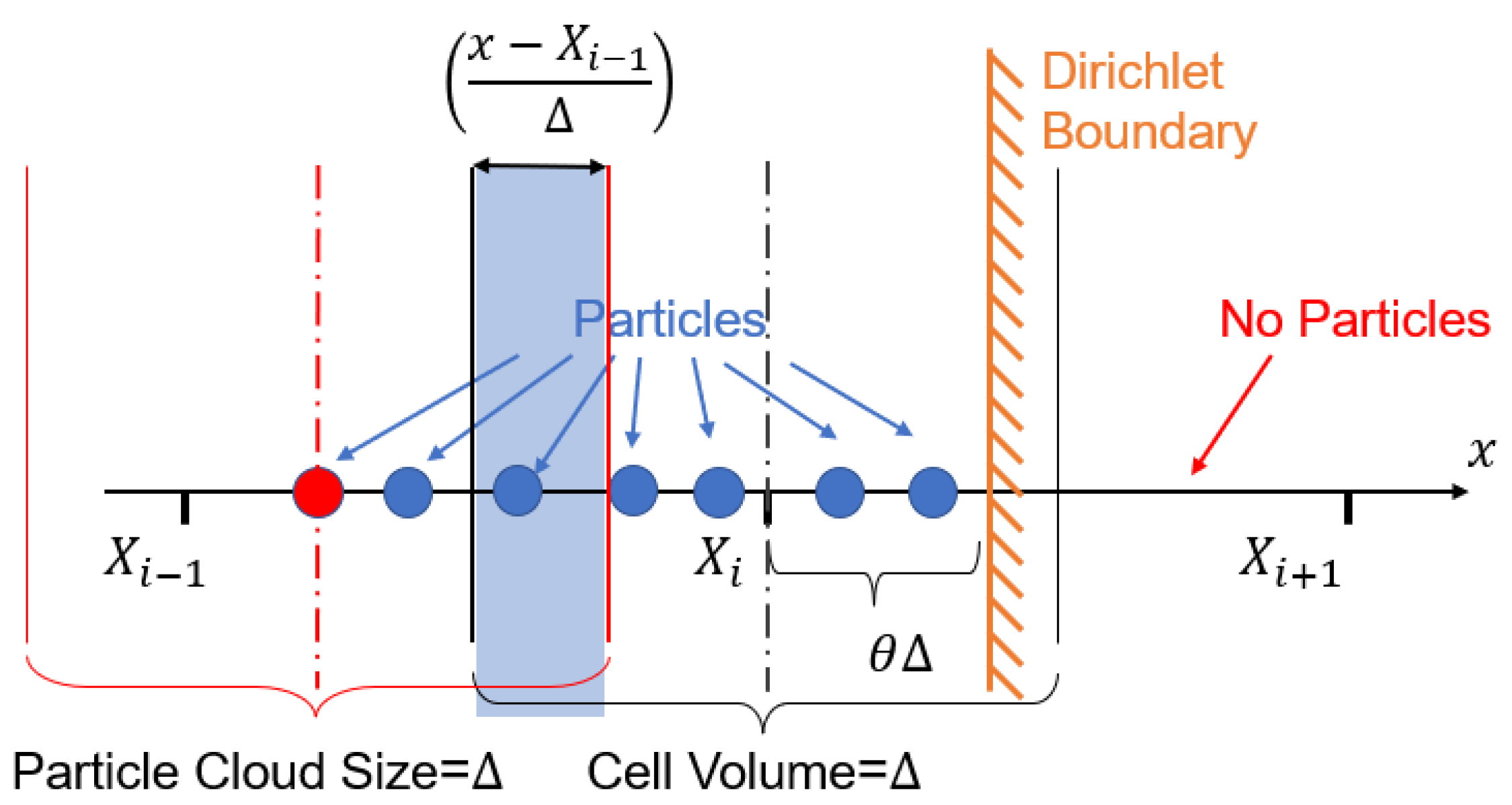
As discussed earlier, the RHS values of the electrostatic Poisson equation in PIC simulations are directly determined by the charge density ρ . For an interior node, this is computed as a weighted average of the electric charges from the surrounding particles, normalized by the cell volume. In standard PIC routines, each particle’s charge is distributed to the nearby grid nodes using first-order weighting—equivalent to a linear interpolation. In 1D settings, for example, the red particle in Figure 2 deposits ( x X i 1 ) / Δ of its charge to node i, with the remainder assigned to node i 1 . The total charge deposited at a node is obtained by summing the contributions from all nearby particles. This sum is then divided by the cell volume to yield the charge density ρ . For 2D problems, this standard process [1] could be formulated into the following equation:
ρ i , j = k q k 1 | x k X i , j | Δ 1 | y k Y i , j | Δ / Δ 2 ,
where ρ i , j denotes the charge density at node ( i , j ) , q k is the charge carried by the k-th particle, and ( X i , j , Y i , j ) are the coordinates of the node. However, this approach becomes inaccurate near Dirichlet boundaries when a node lies within one grid spacing of the boundary. In such cases, the node’s effective deposition volume is truncated by the boundary interface—beyond which no particles exist—leading to an underestimation of both the charge density ϕ and the corresponding RHS value b. This could significantly affect the overall solution accuracy.
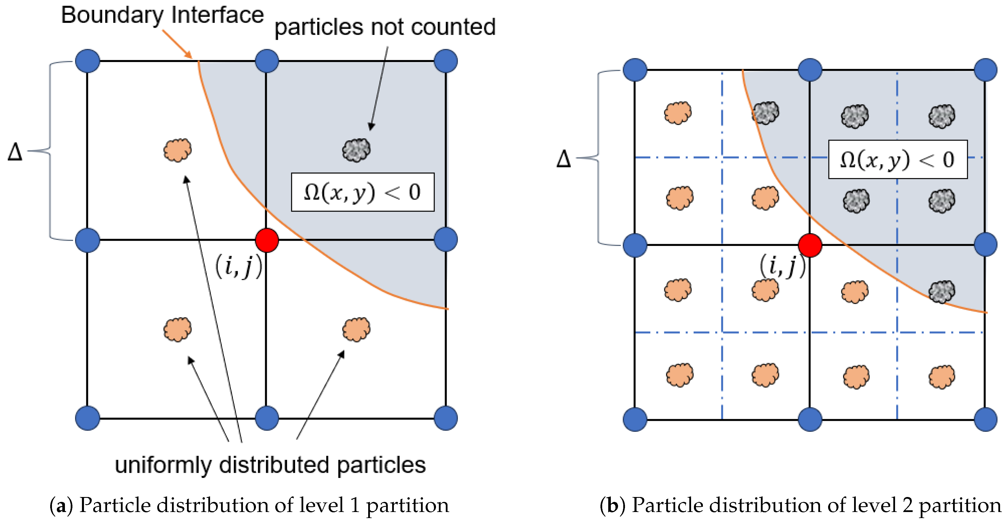
To analyze the impact of these RHS inaccuracies, we designed a numerical procedure that emulates the typical RHS errors arising in PIC simulations at near-boundary nodes. For interior nodes free of RHS inaccuracies, their RHS values are computed directly from the exact solution by taking 2 ϕ ( x ) . For near-boundary nodes, however, we apply a similar sampling process described in Equation (5). To start, the Dirichlet boundary interface is defined explicitly by a level-set function Ω ( x ) = 0 , where Ω < 0 indicates the exterior and Ω 0 defines the interior computational domain. Figure 3 illustrates this setup in 2D. For a near-boundary node ( i , j ) (indicated by the solid red circle), instead of using the exact RHS value, we populate its nearby cells with virtual “particles” to allow for the sampling process. These “particles” are fixed in position, located at subcell centers. The total number of virtual “particles” is determined by the partition level l: node ( i , j ) is associated with 2 2 l particles in 2D, and 2 3 l in 3D. The total number of virtual “particles” is determined by the partition level l: node ( i , j ) is associated with 2 2 l particles in 2D, and 2 3 l in 3D. For example, a partition level of l = 3 corresponds to 2 6 = 64 sampling points per near-boundary node in 2D and 2 9 = 512 sampling points in 3D. For each “particle”, its exact RHS value b k is evaluated at its location, then its contribution to node ( i , j ) ’s RHS is computed by the same first-order weighting. Summing over all contributions yields the approximated RHS value b i , j ¯ , calculated as follows:
b i , j ¯ = k = 1 2 D l 1 2 D ( l 1 ) b k 1 | x k X i , j | Δ 1 | y k Y i , j | Δ ,
where the overline in b i , j ¯ indicates that this value is approximated (inaccurate), D is the spatial dimension (e.g., D = 2 for 2D problems), and b k is the exact RHS value at the k-th particle location. Only particles that lie within the computational domain ( Ω   0 ) are included in the summation, thereby replicating the physical absence of charge beyond the boundary. For 1D and 3D cases, the weighting terms in Equation (6) should be adjusted accordingly to accommodate the dimensionality. When the RHS varies linearly in the vicinity of node ( i , j ) , the procedure in Equation (6) yields the same result as Equation (5). This condition is approximately satisfied when the grid spacing Δ is sufficiently small, such that the RHS can be locally approximated by a linear function, and when the partition level l is sufficiently large, providing adequate sampling resolution for the numerical averaging process. The combined effects of grid refinement and increased partition level improve the accuracy of the reconstructed RHS. In this study, we adopt a partition level of l = 3 for all numerical experiments, which provides a good balance between sampling accuracy and computational cost. The adequacy of this choice is quantitatively validated by the numerical results presented in a later section. Overall, this treatment provides a controlled and physically consistent means of reproducing the RHS underestimation observed in standard PIC routines near boundaries.
To facilitate subsequent error analysis, we define a parameter δ as the ratio between the inaccurate and accurate RHS values at a node, i.e., δ = b ¯ / b . Apparently, δ i , j lies within the range ( 0 , 1 ] . In later numerical tests where the true RHS values b i , j are known, the corresponding δ i , j values can be computed directly from this definition. However, in practical PIC simulations, the exact RHS distribution is not available a priori. Therefore, some assumption about the b ( x ) distribution must be made to estimate an approximated δ i , j ¯ . In our approach, we assume a locally uniform distribution of b ( x ) in the vicinity of node ( i , j ) . The parameter δ i , j (and its approximation δ ¯ ) is implicitly tied to the boundary geometry, represented by the level-set function Ω ( x ) , making direct computation difficult. Nevertheless, in the 1D scenario illustrated in Figure 2, δ i could be derived explicitly by the charge deposition integrals over the truncated cell volume. Specifically, we have
δ i = b i ¯ / b i = X i 1 X i b ( x ) · x X i 1 Δ d x + X i X i + θ Δ b ( x ) · X i + 1 x Δ d x Δ / b i ,
where b ( x ) is an abstract (unknown) RHS distribution function, and the boundary truncates the cell at a distance θ Δ from node i. Assuming b ( x ) is locally uniform b ( x ) yields a closed-form expression for the approximated ratio:
δ i ¯ = 1 2 θ 2 + θ + 1 2 .
This expression is intuitive when considering the limiting cases. For θ = 0 , the Dirichlet boundary lies exactly at node i, blocking half of the cell’s volume. Accordingly, δ i ¯ = 1 / 2 . For θ = 1 , the boundary lies at the neighboring node i + 1 , and node i behaves as a normal interior node with no volume loss, giving δ i ¯ = 1 , as expected.
In the multidimensional (2D or 3D) setting, we extend the same idea used in the 1D case to compute the approximated coefficient δ i , j ¯ (or δ i , j , k ¯ in 3D) for near-boundary nodes. Specifically, we apply the same numerical procedure used in the RHS computation process (as described in Equation (6)), but under the assumption that b ( x ) is locally uniform. In 2D problems, for example, we subdivide the four neighboring cells surrounding a near-boundary node ( i , j ) into smaller subcells and place particles at the center of each subcell, illustrated in Figure 3, following the same sampling strategy as in the actual RHS computation. Each particle is assigned a constant RHS value (i.e., b k = b for some arbitrary constant b), so the resulting computed value b i , j ¯ represents only a fraction of the full uniform value. This fraction, by construction, corresponds to the approximated coefficient δ i , j ¯ , and it can be evaluated using the following expression:
δ i , j ¯ = b i , j ¯ / b = k = 1 2 D l 1 2 D ( l 1 ) 1 | x k X i , j | Δ 1 | y k Y i , j | Δ ,
where b i , j ¯ denotes the value computed using the assumed uniform distribution, and the summation spans all particle contributions within the neighboring region whose positions satisfy Ω 0 , ensuring that only particles located inside the physical domain are counted. This construction allows us to numerically capture the influence of irregular geometry on the RHS evaluations at boundary-adjacent nodes, despite the lack of an explicit form for δ i , j ¯ in terms of θ x and θ y .

3. Error Analysis

3.1. One-Dimensional Error Analysis

We extend the earlier 1D error analysis [26] to account for inaccuracies of RHS values b i ¯ in both the linear and quadratic embedded finite difference schemes. Consider the 1D Poisson equation posed on a domain [ a , b ] with Dirichlet boundaries located at x L and x R . The domain is discretized using N + 1 uniformly spaced grid points such that a = x 0 < x L < x 1 < x 2 < · < x N 1 < x R < b = x N . The fractional distances from x L and x R to their respective adjacent grid nodes are denoted by θ L and θ R , with x L x 1 = θ L Δ x and x N 1 x R = θ R Δ x .
Let the numerical error at node i be defined as ξ i = ϕ i ϕ i e , where ϕ i is the numerical solution and ϕ i e is the exact solution. The local truncation error τ i is defined, following Jomaa and Macaskill [26], as
τ i = b i ( L ϕ e ) i ,
where L denotes the discrete Laplacian operator, which corresponds to the standard second-order central difference scheme for interior nodes. At the two near-boundary nodes i = 1 and i = N 1 , b ¯ i is used instead of the exact RHS, and L must be adjusted based on whether the linear or quadratic embedded scheme is employed. A crucial relation between numerical error ξ and truncation error τ was established by Jomaa and Macaskill [26] as
( L ξ ) i = τ i = H i + 1 / 2 H i 1 / 2 Δ x , 1 i N 1 ,
where H is a first-order difference operator acting on ξ , defined as follows:
H i 1 / 2 = ξ i ξ i 1 Δ x .
Note that at the domain boundaries, H 1 / 2 and H N 1 / 2 are defined consistently with the chosen boundary discretization scheme used for ϕ .

3.1.1. The Linear Scheme Case

For interior nodes, the truncation error is obtained via Taylor expansion:
τ i = Δ x 2 12 ϕ i ( 4 ) + O ( Δ x 4 ) , 2 i N 2
which is a second-order term. Without considering the RHS inaccuracies, the truncation errors at the near-boundary nodes are as follows:
τ 1 = 1 2 ( 1 θ L ) ϕ 1 + O ( Δ x )
and
τ N 1 = 1 2 ( 1 θ R ) ϕ N 1 + O ( Δ x ) ,
both being zeroth-order.
When incorporating RHS inaccuracies and assuming a uniform b ( x ) distribution, the truncation error at node 1 becomes the following:
τ 1 = b 1 ¯ ( L ϕ e ) 1 = b 1 ( L ϕ e ) + δ 1 b 1 b 1 = 1 2 ( 1 θ L ) ϕ 1 + ( δ 1 1 ) b 1 + O ( Δ x ) .
And by substituting δ 1 from Equation (8) and realizing b 1 = ϕ 1 , we have
τ 1 = θ L θ L 2 2 ϕ 1 + O ( Δ x ) ,
which is still a zeroth-order term. Similarly, for the right boundary:
τ N 1 = θ R θ R 2 2 ϕ N 1 + O ( Δ x )
The above relations enable us to write all the numerical error terms to ξ 1 as follows:
ξ i = ξ 1 + ( i 1 ) Δ x H N 1 / 2 Δ x 2 j = 1 i 1 k = j + 1 N 1 τ k . 2 i N 1
To close the set of equations, the left boundary treatment is needed, treated with the linear scheme described in Equation (3) by
H 1 / 2 = ξ 1 ξ L θ L Δ x = ξ 1 θ L Δ x ,
where ξ L = ϕ L ϕ L e = 0 by definition. Similarly, the linear treatment at the right boundary is applied as follows:
H N 1 / 2 = ξ R ξ N 1 θ R Δ x = ξ N 1 θ R Δ x .
Solving these equations finally results in the following:
ξ i = Δ x 2 i + θ L 1 N + θ L + θ R 2 1 k = 1 N 1 ( k + θ L 1 ) τ k k = i + 1 N 1 ( i k ) τ k .
This explicit formula expresses the numerical error ξ i with all the truncation error terms.
To isolate the impact of the left Dirichlet boundary, we set θ R = 1 and consider only τ 1 :
ξ i L = i N 1 θ L τ 1 Δ x 2 i N 1 θ L 2 ( 1 θ L ) 2 ϕ 1 Δ x 2 ,
where τ 1 retained only the highest order term. Apparently, the left boundary induced error component is also a second-order in Δ x , linearly decreasing from left to right. By taking the derivative, we found that the maximum error occurs θ L = 2 / 3 (without RHS inaccuracies, this value was found to be 1 / 2 [26]). Similarly, for the right boundary, we have the following:
ξ i R = i N θ R τ N 1 Δ x 2 i N θ R 2 ( 1 θ R ) 2 ϕ N 1 Δ x 2 ,
which is also second-order in Δ x and peaks at θ R = 2 / 3 . From the above expressions, we also observe that the boundary-induced error components ξ i L and ξ i R consistently have signs opposite to those of the corresponding boundary truncation errors τ 1 and τ N 1 .
The contribution from interior nodes can be approximated by the following integral [26]:
ξ i i n Δ x 2 12 [ x L x i x ϕ ( 4 ) ( x ) d x x i x L x R x L x L x R x ϕ ( 4 ) ( x ) d x + x L x i x L x R x L x L x R ϕ ( 4 ) ( x ) d x x L x L x i ϕ ( 4 ) ( x ) d x + ( x i x L ) x i x R ϕ ( 4 ) ( x ) d x ] ,
which is also second-order in Δ x . Thus, the total numerical error at node i can be approximated as ξ i ξ i L + ξ i R + ξ i i n . This straightforward error decomposition offers a clear and intuitive interpretation of the distinct error contributions in the numerical solution of the Poisson equation.

3.1.2. The Quadratic Scheme Case

Adopting a quadratic scheme improves the truncation errors at the boundaries only, while the truncation errors at interior nodes remain unchanged. In the absence of the inaccurate RHS effect, the truncation errors at the near-boundary nodes τ 1 and τ N 1 are given by
τ 1 = ( 1 θ L ) 3 ϕ 1 Δ x + O ( Δ x 2 )
and
τ N 1 = ( 1 θ R ) 3 ϕ N 1 Δ x + O ( Δ x 2 ) ,
both of which are first-order in Δ x .
As in the analysis of the linear scheme, when RHS inaccuracies are introduced under the assumption of a locally uniform RHS, the boundary truncation errors are significantly altered. For the left boundary, the truncation error becomes the following:
τ 1 = b 1 ¯ ( L ϕ e ) 1 = 1 2 θ L 2 + θ L 1 2 ϕ 1 ( 1 θ L ) 3 ϕ 1 Δ x + O ( Δ x 2 ) ,
which is evidently degraded to a zeroth-order term. A similar derivation for the right boundary yields the following:
τ N 1 = 1 2 θ R 2 + θ R 1 2 ϕ N 1 + O ( Δ x ) .
Following the same approach as in the linear case, we arrive at an equivalent system of equations relating the solution error ξ i and the terms H 1 / 2 and H N 1 / 2 , with the only difference being the updated expressions due to the quadratic boundary treatment (described in Equation (4)):
H 1 / 2 = 2 θ L θ L ξ 1 1 θ L 1 + θ L ξ 2 / Δ x
and
H N 1 / 2 = 2 θ R θ R ξ N 1 + 1 θ R 1 + θ R ξ N 2 / Δ x .
Solving the set of equations leads to the following:
H N 1 / 2 = Δ x { θ L ( 1 + θ L ) 2 τ 1 + [ ( N + θ L 2 ) + θ R ( 1 θ R ) 2 ] τ N 1 k = 2 N 2 ( 1 θ L k ) τ k } / N + θ L + θ R 2 ,
and, consequently:
ξ i = Δ x 2 ( i + θ L 1 ) H N 1 / 2 Δ x 1 2 θ L ( 1 + θ L ) τ 1 + k = 2 N 1 ( 1 θ L k ) τ k k = i + 1 N 1 ( i k ) τ k .
Notably, H N 1 / 2 is now O ( Δ x ) —in contrast to O ( Δ x 2 ) in the absence of RHS inaccuracies [26]—due to the degradation of τ 1 and τ N 1 . As a result, ξ i is uniformly second-order in Δ x , including the boundary nodes ξ 1 and ξ N 1 , which were third-order when the RHS was accurate.
To isolate the left boundary contribution, we set θ R = 1 and retain only the τ 1 term in the above expression, leading to the following:
ξ i L = 1 2 i N 1 θ L ( 1 + θ L ) τ 1 Δ x 2 1 2 i N 1 θ L ( 1 + θ L ) 1 2 θ L 2 + θ L 1 2 ϕ 1 Δ x 2 ,
which varies linearly with i and decreases from the left to the right boundary. Further analysis indicates that the left boundary error is maximized when θ L 0.3904 . Similarly, for the right boundary contribution we obtain the following:
ξ i R = i 2 N θ R ( 1 + θ R ) τ N 1 Δ x 2 i 2 N θ R ( 1 + θ R ) 1 2 θ R 2 + θ R 1 2 ϕ N 1 Δ x 2 ,
which is also linear in i and reaches its maximum at θ R 0.3904 . Again, we observe that the boundary-induced error components ξ i L and ξ i R have signs opposite to those of the corresponding boundary truncation errors τ 1 and τ N 1 . This intriguing behavior also emerges in the 2D cases, as confirmed by later numerical experiments.
From these expressions, we conclude that under the influence of inaccurate RHS values, the quadratic scheme exhibits boundary error contributions of order O ( Δ x 2 ) —qualitatively resembling the behavior of the linear scheme. Meanwhile, the contributions from interior nodes remain O ( Δ x 2 ) and can still be approximated by the integral formula (22). Thus, the simple decomposition ξ i ξ i L + ξ i R + ξ i i n now holds for the quadratic scheme affected by the RHS inaccuracies. In contrast, when the RHS is accurate, the solution error is primarily dominated by the interior contributions [26].

3.1.3. Overview of 1D Error Analysis

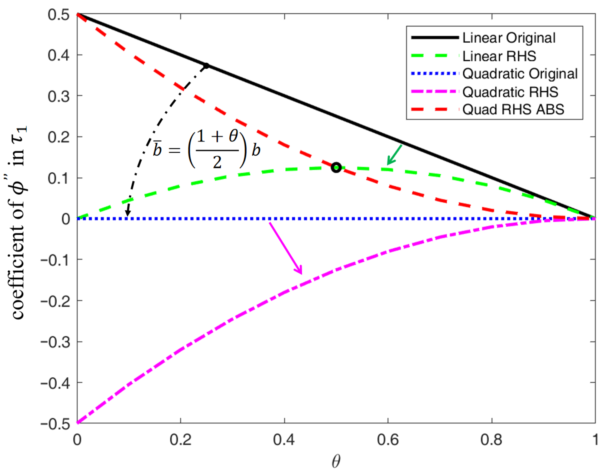
To summarize the 1D error analysis, we begin by comparing the leading-order truncation error at the near-boundary node, specifically the coefficient of ϕ 1 in τ 1 , across four representative scenarios: the linear scheme with and without RHS inaccuracies, and the corresponding quadratic cases. The comparison is illustrated in Figure 4.
For θ ranging from 0 to 1, the presence of inaccurate RHS values reduces the leading truncation error in τ 1 for the linear scheme, while it increases the error for the quadratic scheme. The plot also indicates a special case in which the RHS values are modified as b i ¯ = ( 1 + θ ) / 2 b i in the linear scheme. This modification effectively transforms the linear scheme to the quadratic accuracy, which can be verified via Equations (1), (3), and (4). Notably, the coefficient in the RHS-affected quadratic case has the opposite sign to the linear cases; hence, for comparison, its absolute value is also plotted. The figure shows that for θ ( 0 , 0.5 ) , the RHS-affected linear scheme exhibits a smaller leading error term, whereas for θ ( 0.5 , 1 ) , the RHS-affected quadratic scheme performs better.
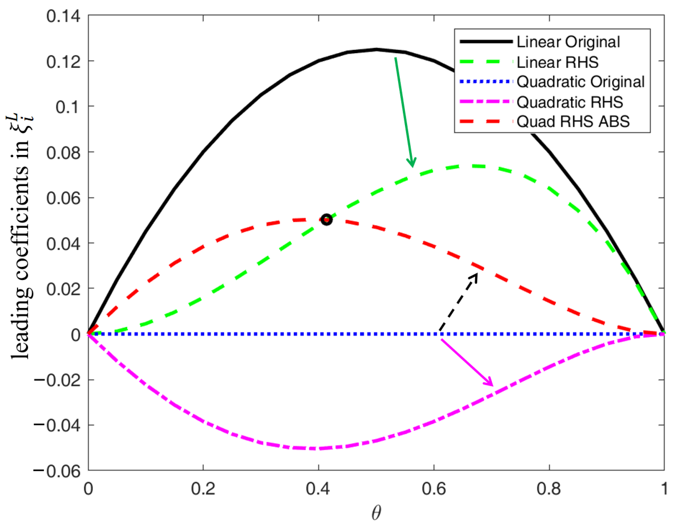
As established in earlier sections, the magnitudes of τ 1 and τ N 1 , in conjunction with θ L and θ R , directly influence the numerical errors ξ i across the domain through the boundary error components ξ i L and ξ i R . Since the interior node contributions remain the same across all schemes, we focus our comparison on the leading-order boundary error terms—specifically, the coefficients of ( i / N 1 ) ϕ 1 Δ x 2 in ξ i L . The results are presented in Figure 5. Note that for the linear scheme unaffected by the RHS inaccuracies, we adopt the ξ i L formula from [26]; for the unaffected quadratic scheme, since the boundary error is third-order (compared to second-order for the remaining cases), it is approximated as zero.
It’s evident that for the linear scheme, boundary errors are reduced across the full range θ ( 0 , 1 ) when RHS inaccuracies are present. In contrast, the quadratic scheme experiences increased boundary errors under the same conditions. Moreover, the boundary error terms for the RHS-affected quadratic scheme and the linear scheme have opposite signs. By comparing the absolute magnitudes of these terms, it is observed that the RHS-affected linear scheme yields smaller boundary errors for θ ( 0 , 0.414 ) , while the RHS-affected quadratic scheme performs better for θ ( 0.414 , 1 ) . Interestingly, this critical θ value is slightly different from that identified in the τ 1 comparison.
In conclusion, the 1D error analysis clearly demonstrates that both the choice of boundary treatment scheme and the RHS inaccuracies significantly influence the numerical solution accuracy for the Poisson equation. These effects manifest primarily by modifying the magnitude and order of the boundary truncation errors τ 1 and τ N 1 , which in turn shape the boundary error components ξ i L and ξ i R . Specifically, RHS inaccuracies tend to improve the linear scheme by reducing the leading truncation errors at boundaries, whereas they degrade the accuracy of the quadratic scheme by introducing zeroth-order error components in the boundary truncation errors.

3.2. Two-Dimensional Error Analysis

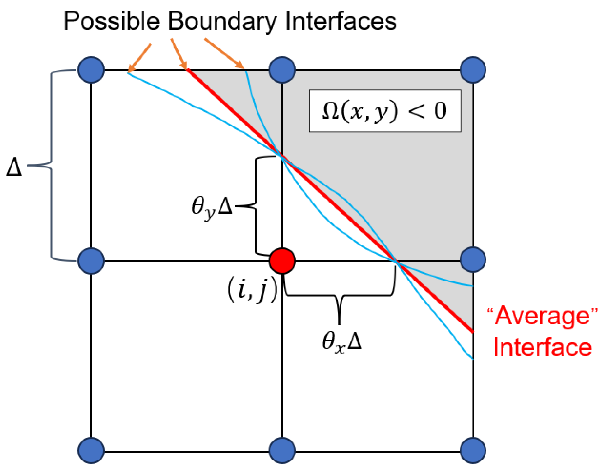
For 2D (or 3D) problems, explicit numerical error expressions are difficult to obtain. Instead, we focus on analyzing how inaccurate RHS values affect the truncation errors at near-boundary nodes. Consider a typical near-boundary node ( i , j ) illustrated in Figure 6, where θ x and θ y represent the relative distances to the boundary along the x- and y-directions, respectively. For a given pair ( θ x , θ y ) , there exist infinitely many possible interface shapes. To enable tractable analysis, we assume that when the mesh spacing Δ is sufficiently small, the “average” interface can be approximated as a straight line uniquely determined by θ x and θ y .
In the absence of RHS inaccuracies, the truncation errors at node ( i , j ) is computed as τ i , j = b i , j ( L ϕ e ) i , j , where the Laplacian operator L acts on both x and y directions. If ( i , j ) is an interior node (i.e., θ x = θ y = 1 ), we can expand ϕ ( x , y ) around the spatial coordinate ( x i , y j ) to obtain the following:
τ i , j = 1 12 4 ϕ x 4 | ( x i , y j ) + 4 ϕ y 4 | ( x i , y j ) Δ 2 + O ( Δ 4 ) ,
which is second-order in Δ . However, when node ( i , j ) is a near-boundary node, the chosen boundary treatment significantly alters the truncation error. Under the linear scheme, the truncation error becomes the following:
τ l i n e a r = 1 θ x 2 2 ϕ x 2 | ( x i , y j ) + 1 θ y 2 2 ϕ y 2 | ( x i , y j ) + O ( Δ ) ,
which is zeroth-order with respect to Δ . If adopting the quadratic scheme, we have the following:
τ q u a d = 1 θ x 3 3 ϕ x 3 | ( x i , y j ) + 1 θ y 3 3 ϕ y 3 | ( x i , y j ) Δ + O ( Δ 2 ) ,
which is first-order.
Now, consider the impact of inaccurate RHS values under the assumption of a locally uniform RHS distribution. For the linear scheme, the truncation error becomes the following:
τ l i n e a r R H S = b i , j ¯ ( L ϕ e ) i , j = b i , j ( L ϕ e ) i , j + δ i , j b i , j b i , j = 1 θ x 2 + δ i , j 1 2 ϕ x 2 | ( x i , y j ) + 1 θ y 2 + δ i , j 1 2 ϕ y 2 | ( x i , y j ) ,
where only leading-order terms are retained. Similarly, for the quadratic scheme, we have the following:
τ q u a d R H S = b i , j ¯ ( L ϕ e ) i , j = δ i , j 1 2 ϕ x 2 | ( x i , y j ) + 2 ϕ y 2 | ( x i , y j ) ,
which now reduces to zeroth-order. From these expressions, it is evident that the quadratic scheme experiences a loss of accuracy due to the degeneration of its boundary truncation error when inaccurate RHS values are present. In contrast, the effect on the linear scheme is more nuanced and depends on the value of δ i , j , which warrants further numerical evaluation.
To this end, we numerically compute the approximate δ i , j ¯ across the full range of θ x and θ y using the method described in Equation (9). We then examine how the coefficients of the 2 ϕ / x 2 and 2 ϕ / y 2 terms in the truncation error are affected in the linear scheme. The results are shown in Figure 7. It can be observed from both Figure 7a,b that, for a given ( θ x , θ y ) pair, RHS inaccuracies tend to improve the linear scheme by reducing the coefficients of the leading-order error terms. Further assuming 2 ϕ / x 2 2 ϕ / y 2 , Figure 7c shows that the RHS-affected linear scheme consistently reduces the boundary truncation error, except for a narrow band where both θ x and θ y are close to 1.
We further compare the boundary truncation errors between the linear and quadratic schemes, both under the influence of inaccurate RHS values. As shown in Figure 8, the RHS-affected linear scheme exhibits uniformly smaller truncation errors than the quadratic scheme across the entire ( θ x , θ y ) domain. However, further numerical experiments are necessary to determine whether this advantage in boundary truncation errors translates to overall improvements in the solution accuracy of the Poisson equation, particularly in scenarios where RHS values are not uniformly distributed.

4. Test Cases and Results

Numerical tests were conducted on a series of 1D, 2D, and 3D examples with predefined analytical solutions ϕ ( x ) . For each test case, the computational domain was embedded in a uniformly spaced Cartesian mesh, and both linear and quadratic boundary treatment schemes were employed to discretize the Poisson equation, yielding a linear system of the form A ϕ = b . The system was solved using a direct solver with row pivoting to reduce rounding errors, rather than iterative solvers. After obtaining the numerical solution, the error vector was computed as ξ = ϕ ϕ e .
While various boundary geometries and analytical forms of ϕ ( x ) were also tested, the results consistently supported the same conclusions. Therefore, for brevity and clarity, we present only three representative examples in this section. The test cases are described as follows.
  • One-dimensional example. Poisson equation is to be solved in a 1D domain [ 0.5 , 0.5 ] with the exact solution given by ϕ ( x ) = 4 x 2 sin 2 π x , which determines the RHS values by b ( x ) = d 2 ϕ / d x 2 = 8 ( 1 2 π 2 x 2 ) sin 2 π x + 32 π x cos 2 π x . Dirichlet boundaries are defined such that | x | 0.313 denotes the outside region. The domain [ 0.5 , 0.5 ] is chosen so that the computational interval has unit length and is centered at the origin, which simplifies grid refinement and yields clearer visualization of the solution and error profiles.
  • Two-dimensional example. The 2D Poisson equation is defined in a square area [ 1 , 1 ] × [ 1 , 1 ] , with an exact solution ϕ ( x , y ) = ( x + 2 ) 2 + ( y 2 ) 2 1 , which has the corresponding RHS values of b ( x , y ) = 2 ϕ = 4 / ( 8 + 4 x + x 2 4 y + y 2 ) 2 . A closed Dirichlet boundary interface is defined by a pair of parameterized equations x ( t ) and y ( t ) , where x ( t ) = 0.02 5 + [ 0.5 + 0.2 sin 5 t ] cos t , and y ( t ) = 0.02 5 + [ 0.5 + 0.2 sin 5 t ] sin t . This Dirichlet interface is shaped like a starfish, whose inside contains all the inner grid nodes. In order to decide whether a grid node ( i , j ) is inside the boundary and to calculate the θ x and θ y if it’s a near-boundary node, it is recommended that the calculations are done in a shifted polar coordinate system originated at ( 0.02 5 , 0.02 5 ) , then any point that is within the radius of ( 0.5 + 0.2 sin 5 t ) is inside the boundary.
  • Three-dimensional example. The 3D Poisson equation is solved within a cubic domain [ 0 , 1 ] 3 , where a spherical boundary decides the inner nodes by Ω < 0 , where Ω ( x , y , z ) = ( x 0.5 ) 2 + ( y 0.5 ) 2 + ( z 0.5 ) 2 0.3 . The exact solution is given by ϕ ( x , y , z ) = exp ( x 2 y 2 z 2 ) , from which the RHS values are computed as b ( x , y , z ) = exp ( x 2 y 2 z 2 ) ( 4 x 2 + 4 y 2 + 4 z 2 6 ) .

4.1. One-Dimensional Numerical Test Results

We numerically solved the 1D Poisson example under four scenarios: using accurate RHS values b i = b ( x i ) and inaccurate RHS values b i ¯ = δ i ¯ b i (with δ i ¯ computed from Equation (8)), each under the linear and quadratic treatments. For each case, we also computed the contributions to the numerical error ξ i from three components: The left boundary ( ξ i L ), the right boundary ( ξ i R ), and the inner nodes ( ξ i in ). Notably, the inner node contribution ξ i in remains unchanged across all cases. These decomposed components were used to validate the approximate relationship ξ i ξ i L + ξ i R + ξ i in , and were plotted together for comparison.
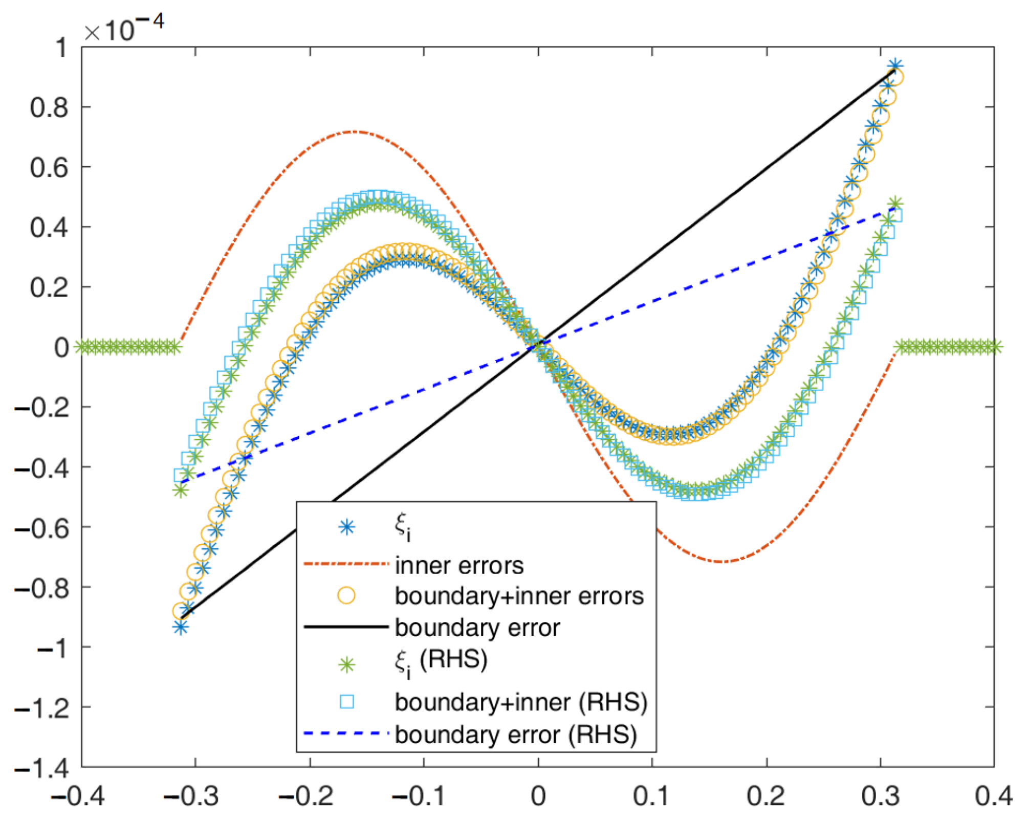
Figure 9 compares the error distributions obtained from the linear scheme with and without RHS inaccuracies. It can be seen that the sum of boundary and inner contributions well approximates the numerical error at each node. By introducing the RHS effect, the boundary contributions (represented by two linear lines) were reduced at all nodes but more evident at the two boundary ends. This reduction directly translates into a lower numerical error at the boundary nodes. In general, the reduced boundary contributions lead to an overall decrease in ξ i at each node. However, it is worth noting that the signs of ξ i L and ξ i R can be opposite to that of ξ i in , as is the case here, slightly complicating the interpretation of error behavior.
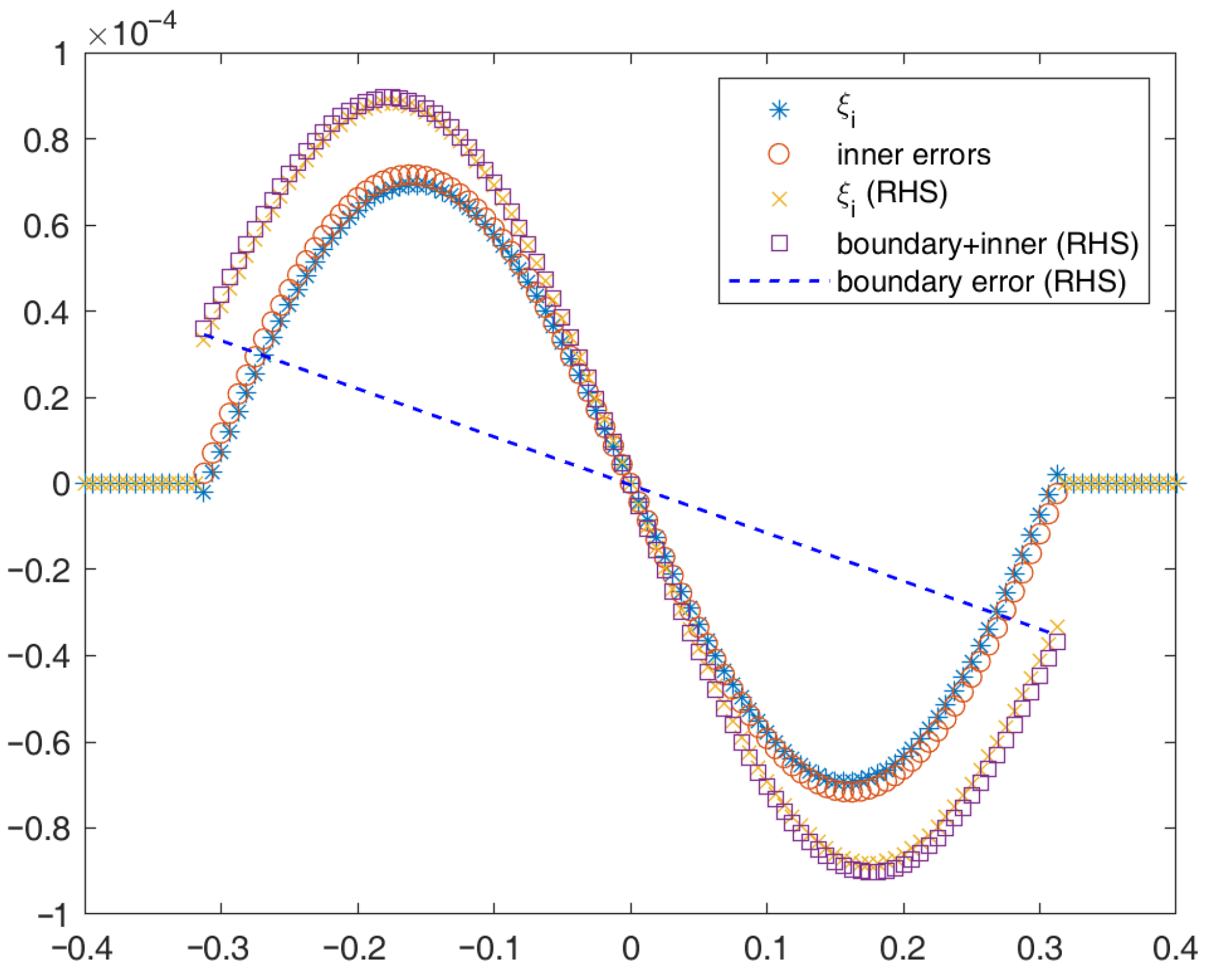
Figure 10 shows a similar comparison for the quadratic scheme. In the RHS-affected case, numerical errors again align with the sum of boundary and inner contributions. Without RHS inaccuracies, the errors are dominated by the inner-node contributions alone. The inclusion of inaccurate RHS values introduces additional boundary error components that vary approximately linearly from the left to the right boundary. Interestingly, the signs of the boundary error contributions in this case are opposite to those in the linear scheme, in agreement with the earlier 1D error analysis. As a result, these boundary terms constructively add to the inner-node contributions, amplifying the total numerical error ξ i throughout the domain.
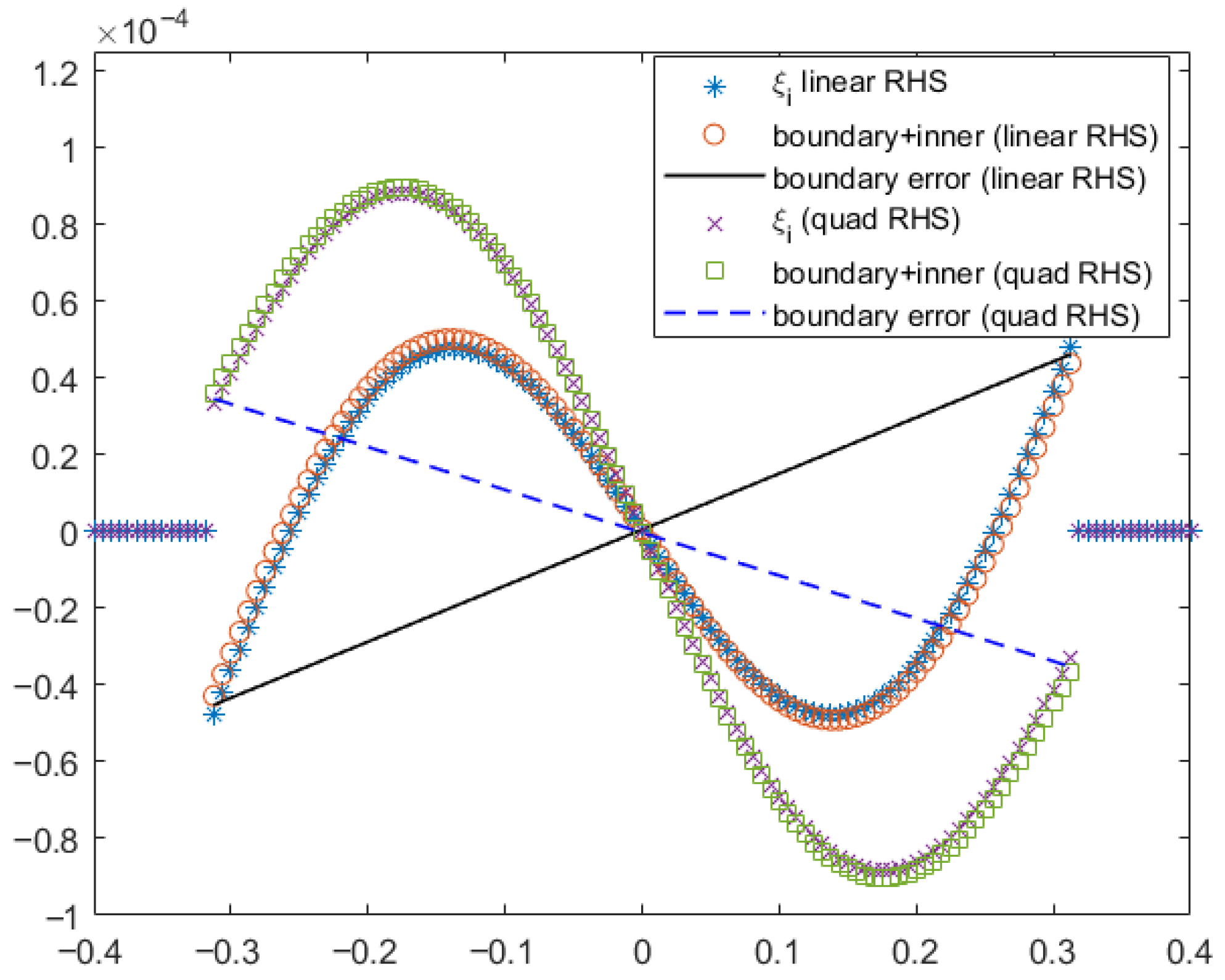
Figure 11 provides a direct comparison of the numerical errors obtained using the linear and quadratic schemes under inaccurate RHS values. Both methods exhibit qualitatively similar behavior: numerical errors arise from additive contributions of boundary and interior nodes. The boundary contributions, ξ i L and ξ i R , are most pronounced near the two boundary ends, where the impact of RHS inaccuracies is most significant. Notably, these boundary-induced errors have opposite signs in the linear and quadratic schemes, consistent with the trends observed in the 1D error analysis.
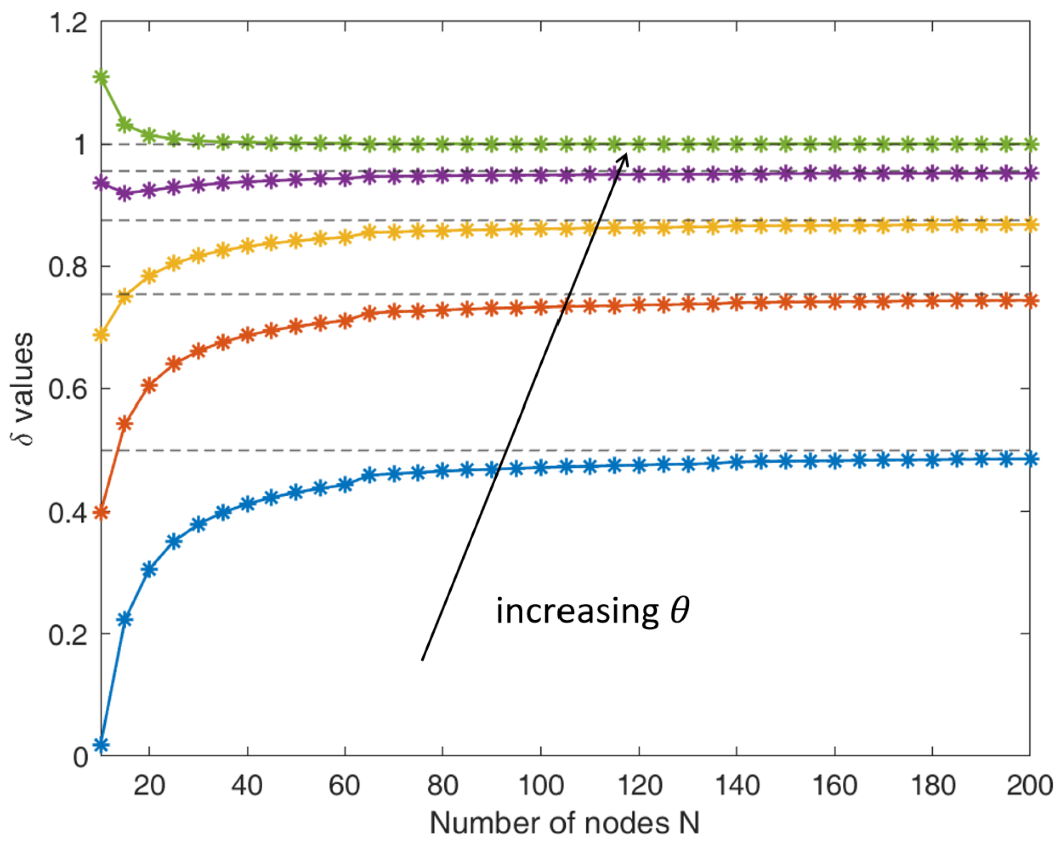
Overall, the 1D numerical tests confirmed the findings from the 1D error analysis in previous sections. We emphasize that for consistency with earlier analysis, the approximated δ i ¯ values used in the tests were computed using Equation (8), rather than the more accurate integral form of Equation (7). This simplification has a negligible effect on the results when Δ x is sufficiently small, as the two expressions yield nearly identical δ i values under such conditions. This agreement is illustrated in Figure 12, which plots both forms of δ i for various choices of θ and Δ x . The close match between the two confirms the validity of using the simpler form in both the numerical experiments and theoretical analysis.

4.2. Two-Dimensional/Three-Dimensional Numerical Tests and Discussions

For the 2D and 3D tests, we followed the same four scenarios as in the 1D case, involving linear and quadratic schemes with and without inaccurate RHS values. For the RHS-affected cases, the modified RHS values b i , j ¯ were computed using Equation (6) at all near-boundary nodes. The corresponding δ i , j ¯ values were obtained as b i , j ¯ / b i , j , where the accurate RHS values b i , j were evaluated from the prescribed b ( x , y ) expression. Due to the lack of explicit analytical expressions for boundary and interior error contributions in higher dimensions, we began by analyzing the truncation errors at near-boundary nodes and compared them with the resulting numerical errors, aiming to identify qualitative correlations. For the 2D case, the full numerical error field was visualized, while for 3D, representative numerical results were summarized in tabular form. Lastly, for RHS-affected cases, we also tested the effectiveness of using approximated δ i , j ¯ values to counteract the impact of RHS inaccuracies.
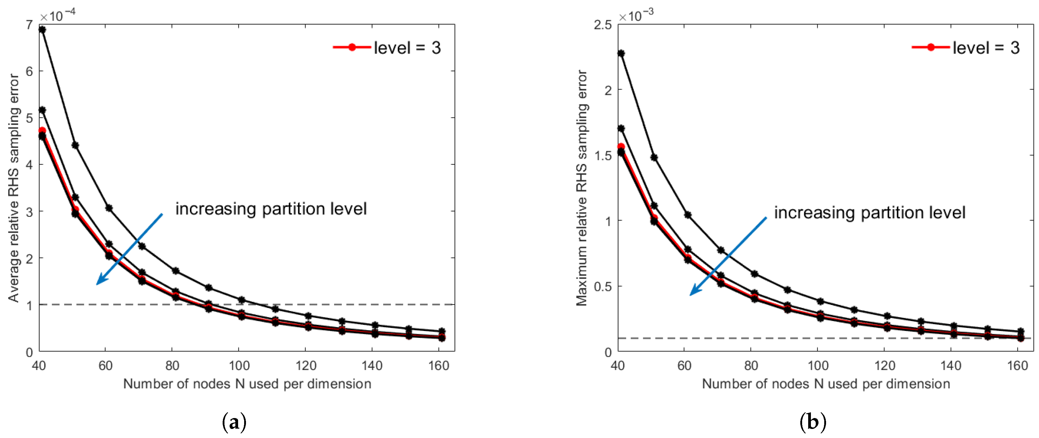
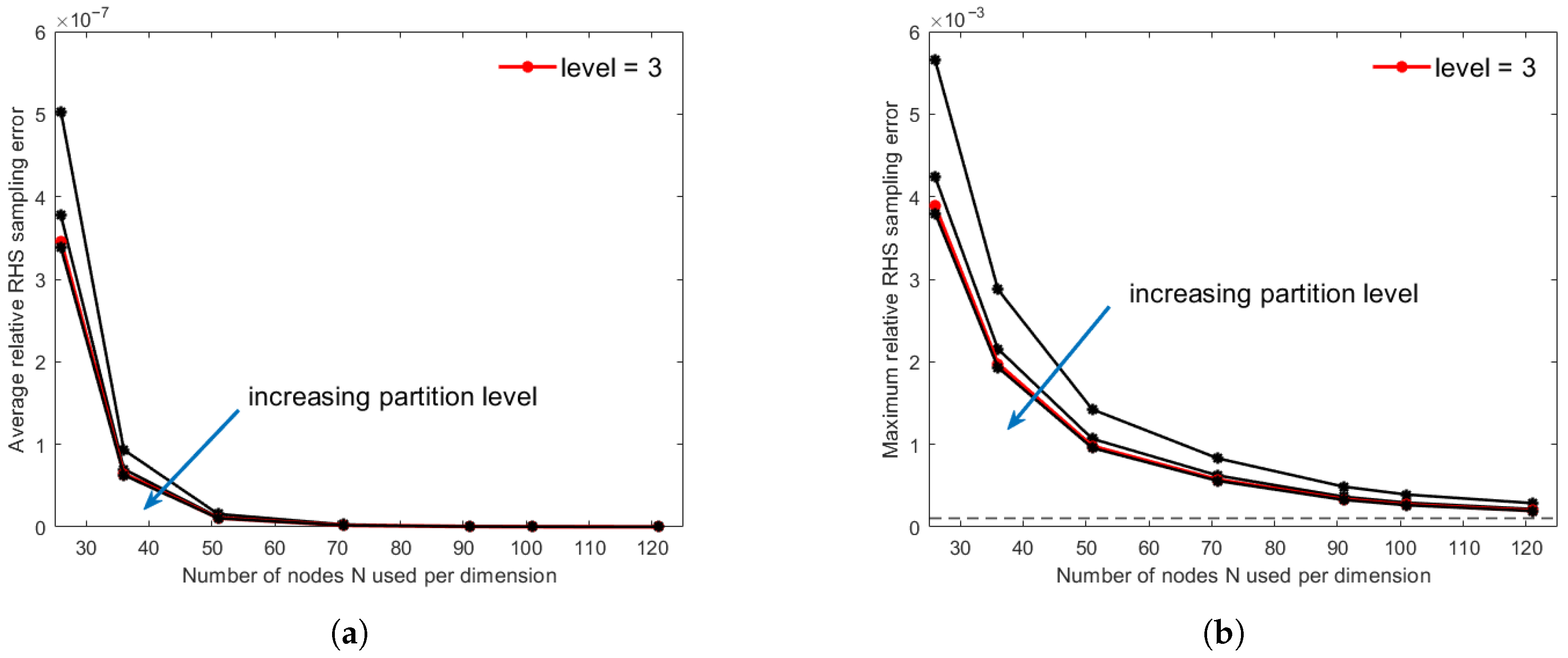
The effects of the partition (sampling) level and grid resolution are illustrated in Figure 13 for the 2D cases and in Figure 14 for the 3D cases. It can be seen that increasing either the partition level or the number of grid points reduces the RHS sampling error. In particular, a partition level of 3 yields results that are essentially indistinguishable from those obtained with higher partition levels, which justifies our choice of level 3 in this study. For the 2D cases, the use of a 151 × 151 grid results in a maximum relative RHS sampling error below 1.0 × 10 4 , which is sufficiently accurate for the purposes of this work. For the 3D case, a grid resolution of 101 3 produces a maximum relative error of 2.696 × 10 4 .

4.2.1. Boundary τ and ξ for the 2D Case

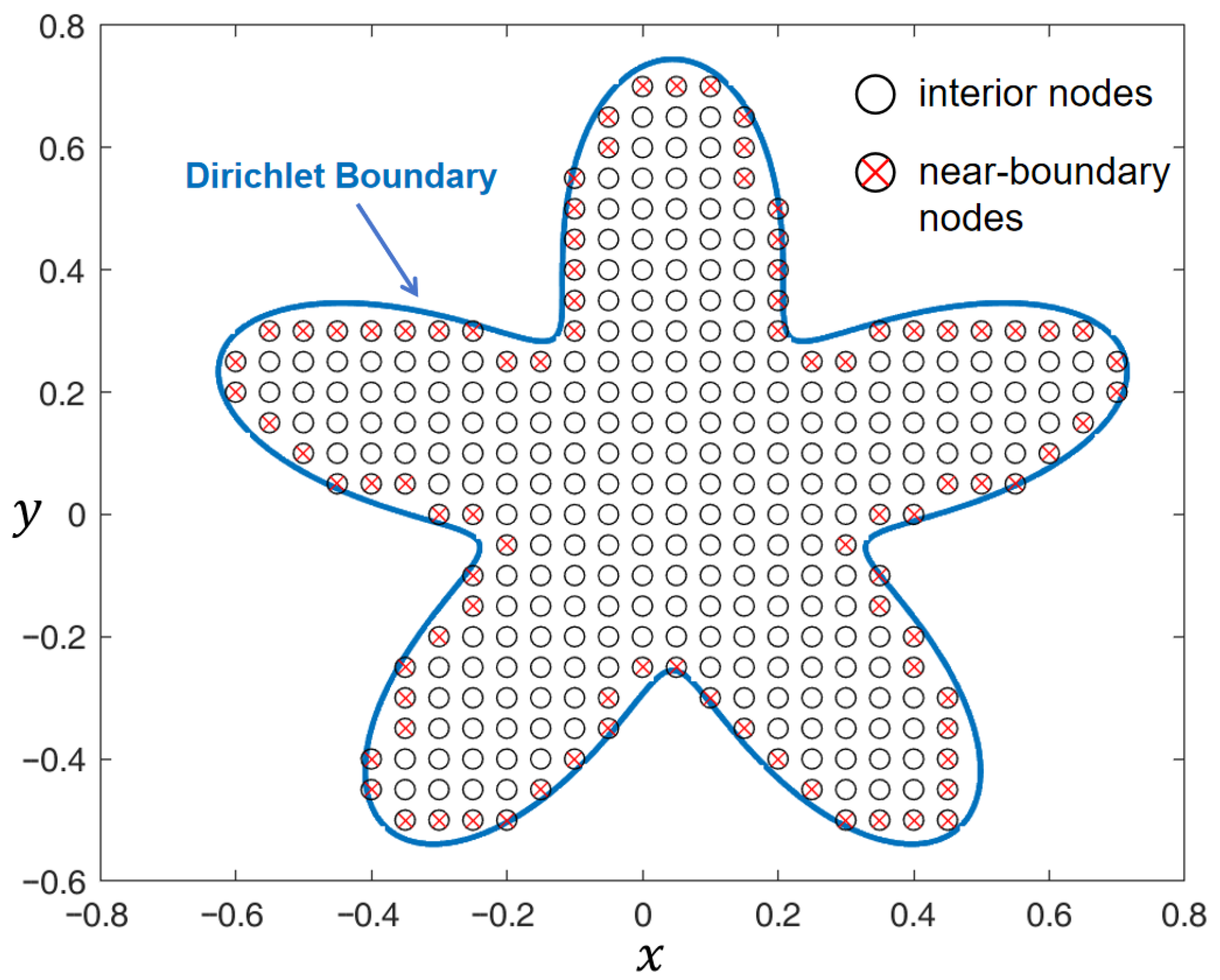
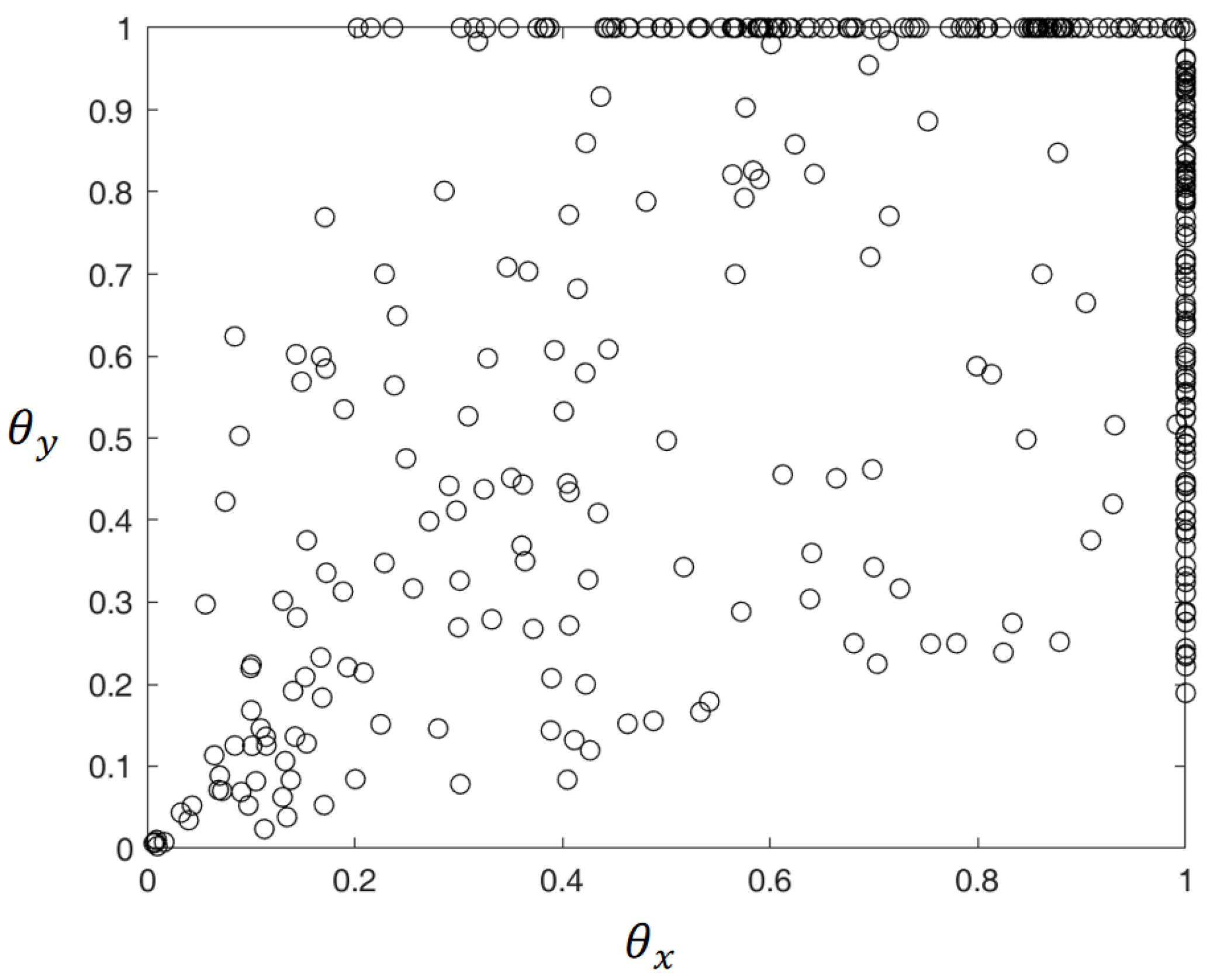
Figure 15 illustrates the computational domain for the 2D case. The solid line denotes the Dirichlet boundary, the open circles indicate the interior nodes, and the circles marked with a cross represent the near-boundary nodes. A total of 41 × 41 nodes are used here for demonstration purposes; however, much finer grids were employed in the actual numerical solution of the 2D Poisson equation. Each near-boundary node is associated with a pair of θ x and θ y values. Figure 16 displays all the θ pairs when a 151 × 151 grid was employed. It is not surprising that the distribution of θ values is non-uniform, as it strongly depends on the shape of the Dirichlet boundary. Notably, a considerable number of near-boundary nodes have either θ x = 1 or θ y = 1 .
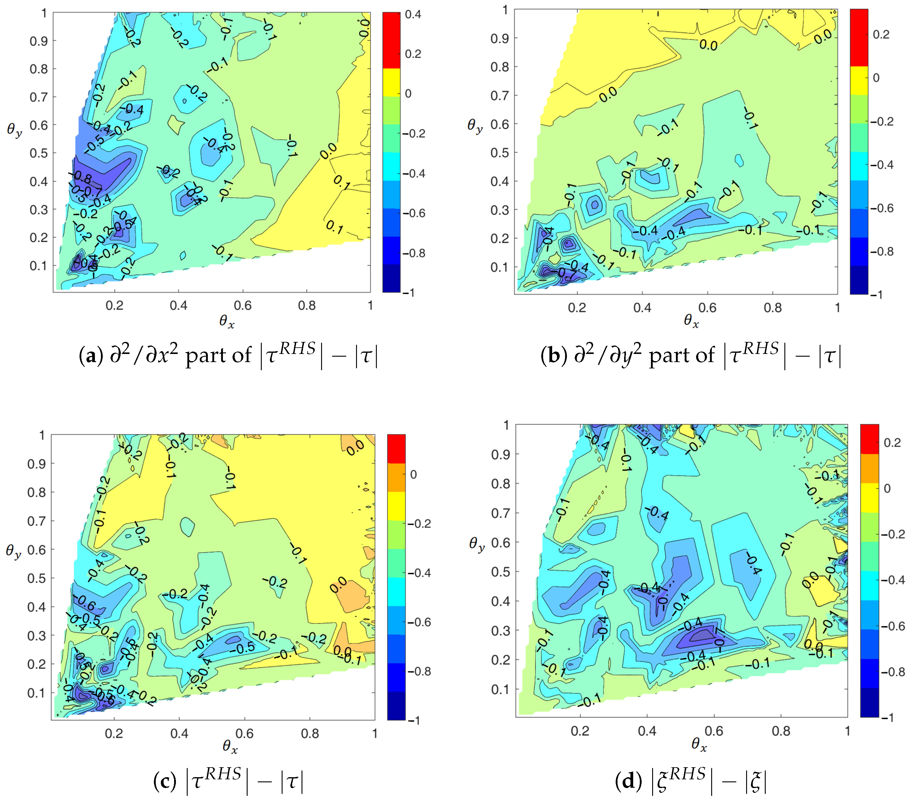
We first investigated the RHS effect on the linear scheme by examining the truncation errors at the near-boundary nodes. The exact solution ϕ ( x , y ) (and thus its second partial derivatives) enables us to compute the leading truncation error terms component-wise using the Equations (32) and (34). Once the computation was done, we made the comparison by evaluating | τ RHS | | τ | at each near-boundary node and plotted the resulting differences as a contour over the θ x and θ y axes. Correspondingly, the numerical error differences | ξ R H S | | ξ | between the RHS-affected and the original linear scheme case at the near-boundary nodes were also computed and compared.
Figure 17 presents these contour plots, where the results were normalized by their respective maximum absolute values. As shown in Figure 17a, for most ( θ x , θ y ) pairs—except in the lower-right region of the θ domain—the RHS effect reduces the corresponding truncation error components (the 2 / x 2 part). Comparing this contour with Figure 7a, we observe very similar dividing lines (i.e., the zero level curves), which qualitatively validates the 2D error analysis. Likewise, Figure 17b and Figure 17c exhibit patterns similar to those in Figure 7b and Figure 7c, respectively. Finally, Figure 17d compares the numerical errors between the RHS-affected and original linear cases. Clearly, in most of the θ domain—except for small regions enclosed by the zero level curves in Figure 17c—the truncation errors for the RHS-affected linear scheme are smaller. Consequently, the resulting numerical errors also tend to be smaller, as seen from the similar zero-level region in Figure 17d. These results suggest that the RHS effect generally improves the linear scheme by reducing truncation errors at near-boundary nodes, and thus also reducing the numerical errors at those near-boundary nodes.
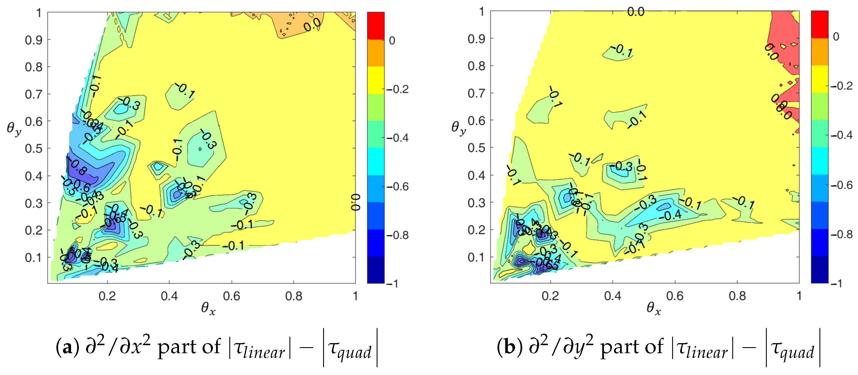
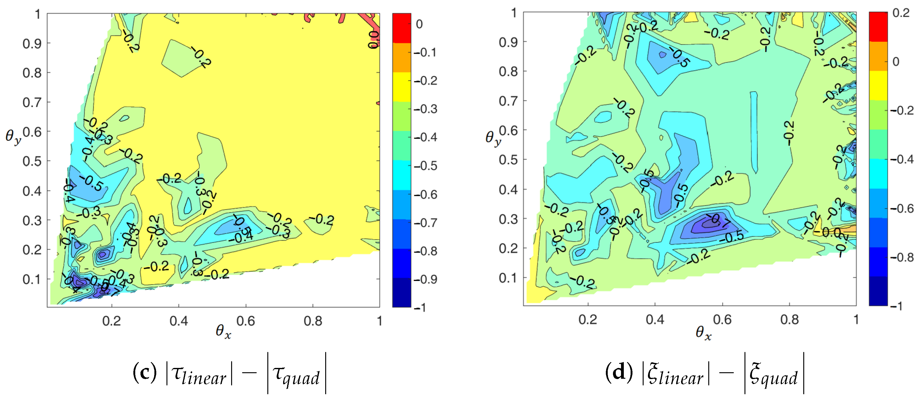
Next, we performed similar comparisons between the RHS-affected linear and RHS-affected quadratic cases. Figure 18 presents these results. As seen from Figure 18a–c, the RHS-affected linear scheme yields smaller truncation errors for almost all the ( θ x , θ y ) pairs compared to the RHS-affected quadratic scheme. These findings are consistent with the earlier analysis presented in Figure 8a–c, which showed that the linear scheme outperforms the quadratic scheme in terms of truncation errors at near-boundary nodes under RHS effects, assuming locally uniform RHS distribution and “average” boundary shapes. It is also important to compare the resulting numerical errors at all near-boundary nodes, as shown in Figure 18d. Once again, the results support the conclusion that smaller truncation errors generally lead to smaller numerical errors at near-boundary nodes.

4.2.2. Global Accuracy Assessment and RHS Error Compensation

To quantify the numerical errors for each case, we measured the L 1 and L norms of the numerical error vector ξ . The L 1 norms were normalized by the number of inner nodes to represent the “average” error of the numerical solution, whereas the L norms represent the maximum errors. Using the error results obtained from different node spacing Δ 1 and Δ 2 , we could estimate the error order p, using the formula p = ln ( L Δ 1 / L Δ 2 ) / ln ( Δ 2 / Δ 1 ) . For each case, we listed these quantities in table form and then juxtaposed the plots of the truncation errors and the resulting numerical errors at all nodes.
We first present the accuracy results for solving the 2D problem using both the linear and quadratic schemes, without the effect of an inaccurate RHS. Table 1 summarizes the numerical error results, tested on different meshes. It is observed that as the number of nodes increased, both the linear and quadratic schemes exhibited second-order accuracy, although the errors were consistently lower for the quadratic setup, particularly in the L norm. However, when the number of nodes reached 161 × 161 , the solution quality suddenly dropped in the quadratic case, despite the finer mesh grids. Further investigation revealed that this phenomenon occurs whenever an inner node is situated between two Dirichlet boundary interfaces along a specific axial direction (i.e., it has no neighboring nodes along that direction). In such cases, while the quadratic scheme remains applicable, it generates substantial truncation errors at these nodes, thereby degrading the overall solution accuracy. To avoid this issue, some detection measure must be employed, and the treatment of these “troubled” nodes should revert to the linear scheme to prevent failure due to insufficient stencil points. Once corrected, the resulting L 1 and L norms were reduced to 1.508 × 10 8 and 6.131 × 10 8 , respectively. This indicates that the quadratic scheme is less robust than the linear one. For this reason, later (and earlier) numerical error plots were generated on a 151 × 151 mesh, where such a situation is absent.
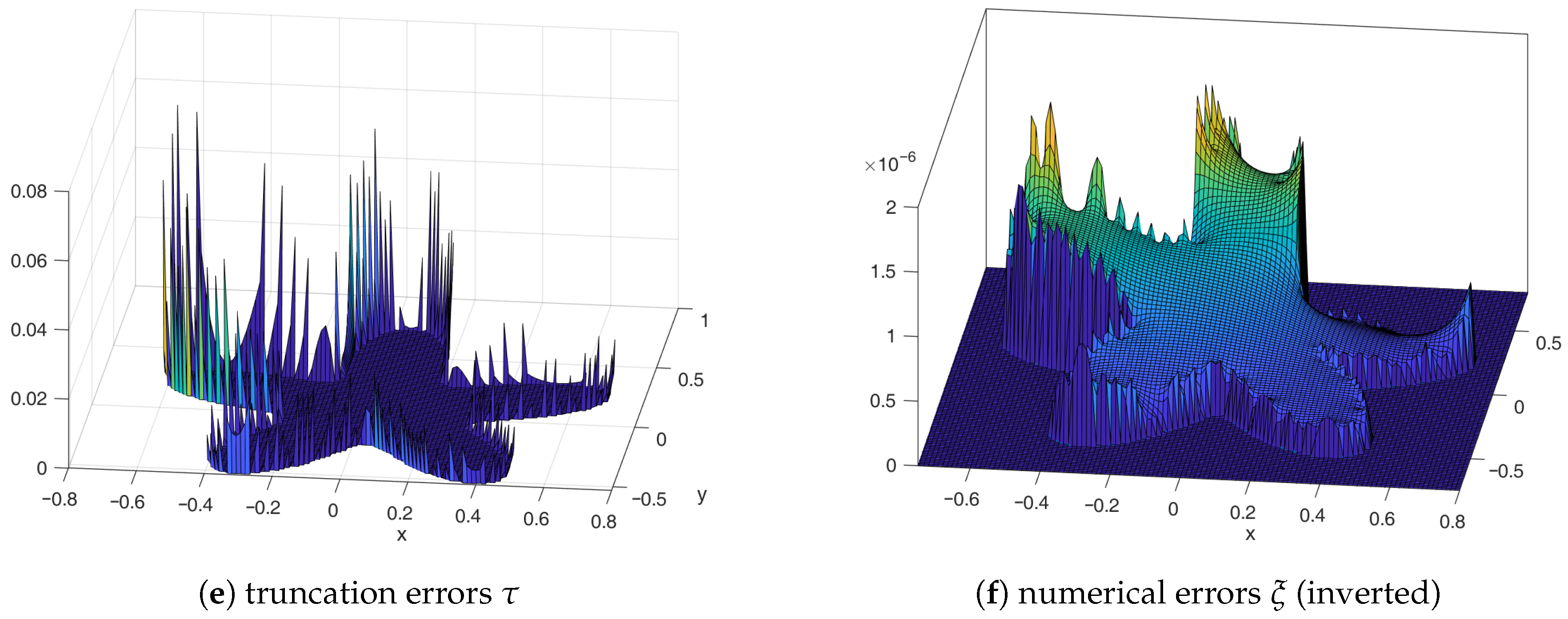
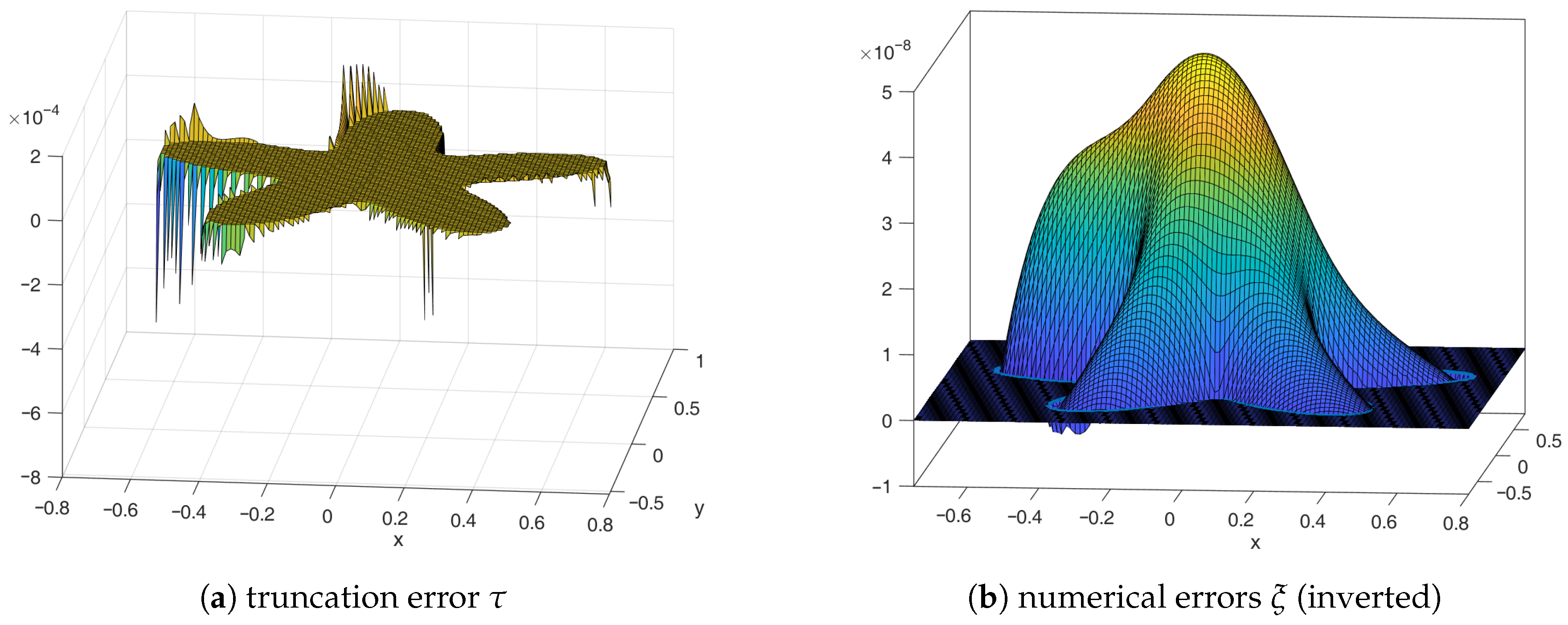
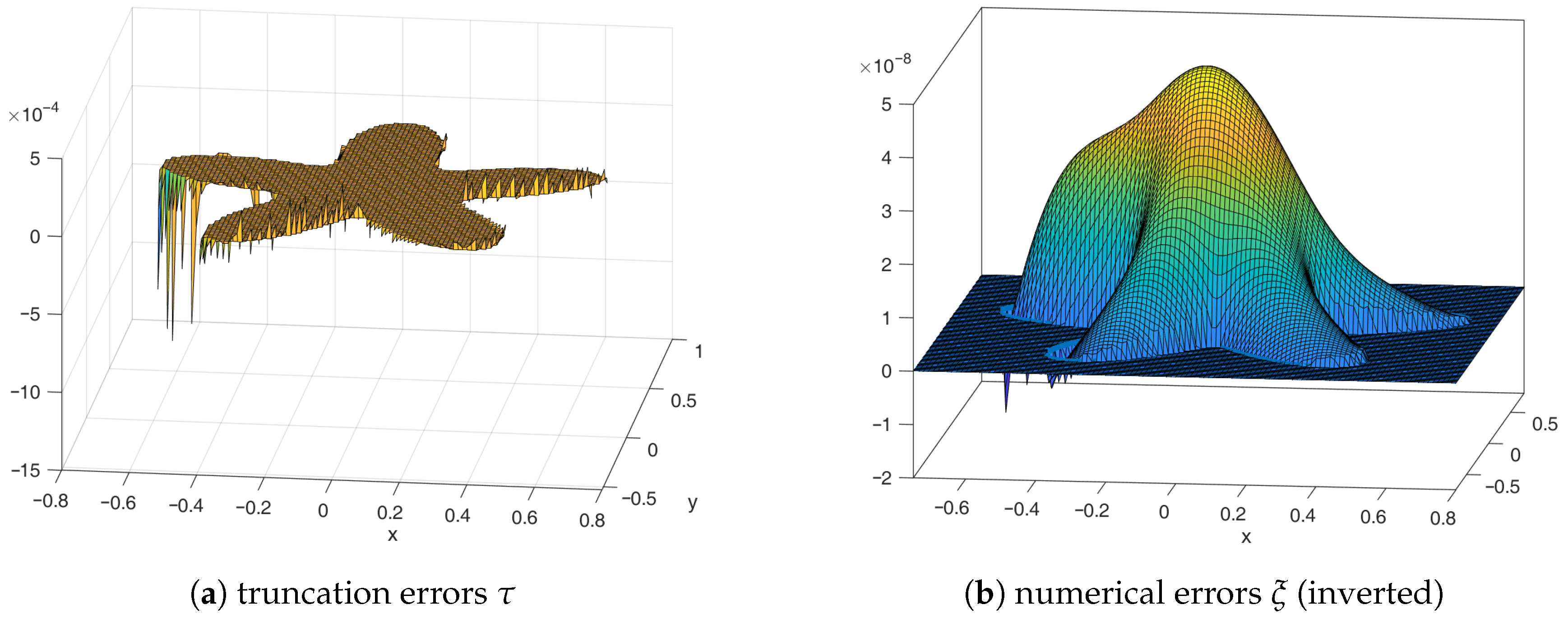
Figure 19 presents the truncation and numerical errors at all nodes obtained from solving the 2D Poisson equation using the linear scheme with accurate RHS values. As shown in Figure 19a, the truncation errors near the boundary—being zeroth-order—are significantly larger than those in the interior, which are second-order. Consequently, the numerical errors in Figure 19b are most pronounced at the boundaries and decrease smoothly in magnitude toward the interior of the domain. Figure 20 shows the corresponding errors obtained using the quadratic scheme with accurate RHS values. As illustrated in Figure 20a, although the truncation errors—now first-order—remain larger near the boundaries, their magnitudes are substantially reduced compared to those in the linear scheme. This reduction results in a qualitatively different numerical error distribution, which now exhibits a center-dominant pattern, as seen in Figure 20b. Note that, based on previous 1D error analysis showing that boundary truncation errors and numerical errors have opposite signs, the numerical error plots herein have been inverted to facilitate direct visual comparison with the corresponding truncation error plots.
Next, we present the results for the two-dimensional case in the presence of the inaccurate right-hand side (RHS) effect. The numerical errors are summarized in Table 2. It can be observed that both the linear and quadratic schemes retain second-order accuracy. However, upon examining the L 1 and L error magnitudes between the two schemes, it could be seen that the RHS-affected linear scheme consistently outperformed those of the quadratic counterpart. Moreover, when these results are compared with those in Table 1, it becomes evident that the linear scheme benefits from the use of the inaccurate RHS values b i , j ¯ , whereas the quadratic scheme experiences a notable degradation in accuracy. These findings extend the previous analysis by demonstrating that the use of b i , j ¯ not only alters the boundary truncation errors τ , and consequently the boundary numerical errors ξ , but also impacts the overall accuracy across the entire computational domain.
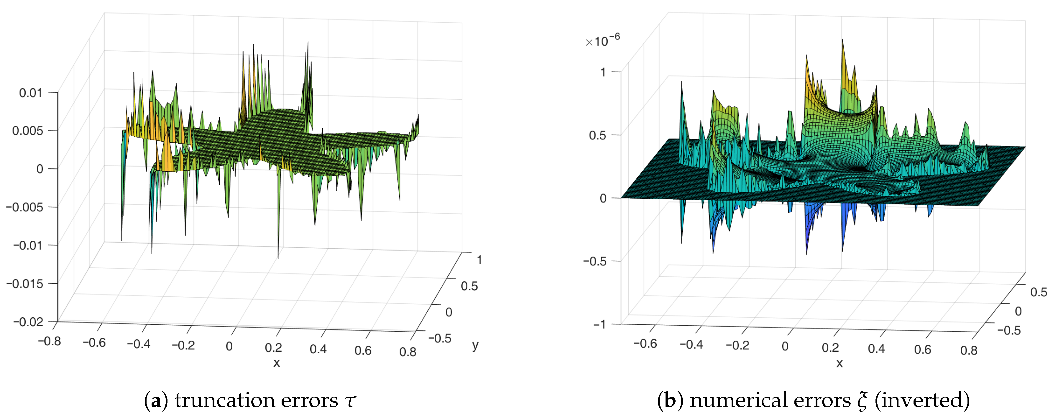
Figure 21 presents the truncation and numerical errors associated with solving the 2D Poisson equation using the linear scheme with inaccurate right-hand side (RHS) values b i , j ¯ . As illustrated in Figure 21a, the truncation errors near the boundaries remain dominant relative to those in the interior; however, their magnitudes are reduced compared to the case with accurate RHS values (see Figure 19a). Notably, the signs of the truncation errors near the boundaries may change at certain nodes. Correspondingly, the numerical errors, shown in Figure 21b, also exhibit an overall reduction in magnitude and sign changes in specific regions.
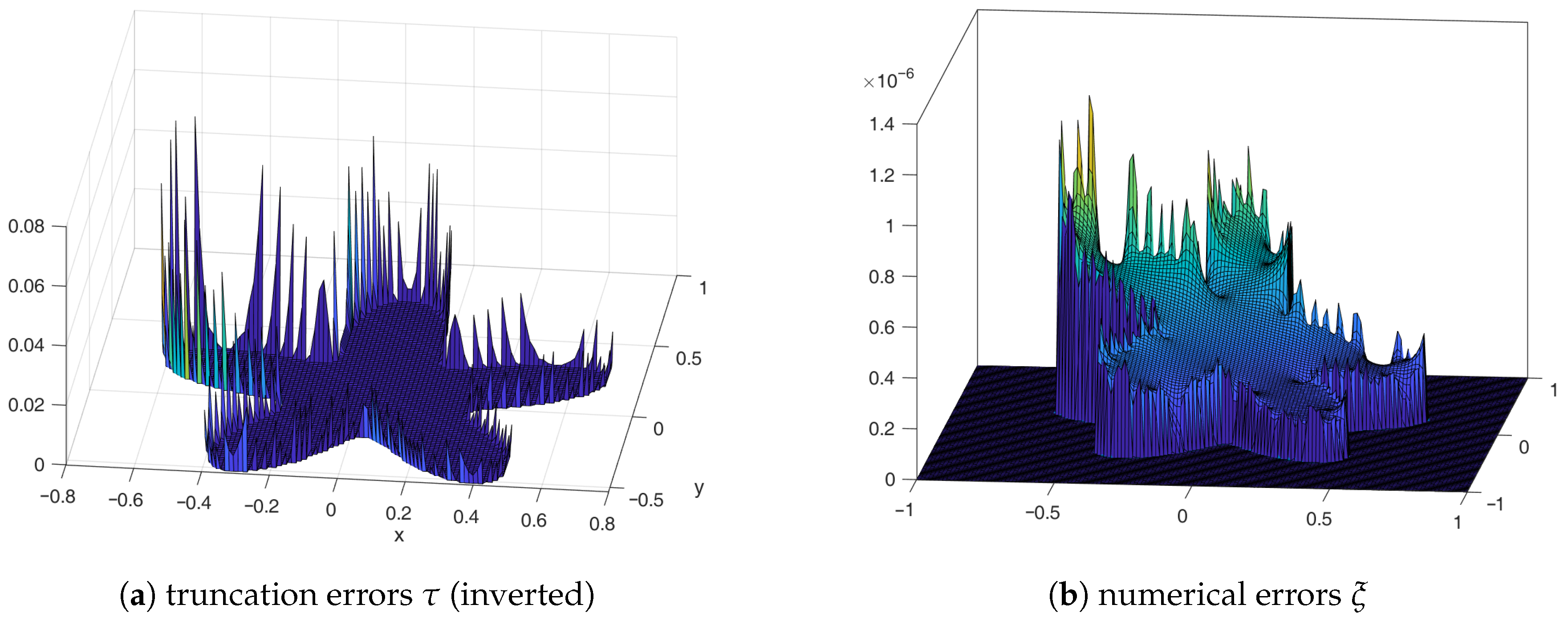
Figure 22 displays the corresponding error plots obtained using the quadratic scheme with the same inaccurate RHS values. For clarity, the truncation error plot is inverted. As evident from Figure 22a, the truncation errors near the boundary are approximately two orders of magnitude larger than those observed in Figure 20a, where accurate RHS values were used. This increase aligns with the earlier 2D error analysis, which indicates that inaccurate RHS values modify the boundary truncation error from a first-order term to a zeroth-order term. Given that the numerical experiments used a grid size of 2 / 150 0.01 , the observed difference in magnitude is consistent with theoretical expectations.
We note that the truncation and numerical error surfaces in Figure 19, Figure 20, Figure 21 and Figure 22 are not smooth, particularly near the Dirichlet boundaries. This behavior is expected and does not improve substantially with finer grids. As seen in Equations (32) and (33), the magnitude of the truncation errors near the boundaries is governed by derivatives evaluated at the boundary interface, which converge to fixed values with grid refinement. Additionally, the coefficients ( 1 θ ) / 2 and ( 1 θ ) / 3 , where θ [ 0 , 1 ] , vary discontinuously across nodes. Consequently, the non-smooth spatial distribution of these coefficients leads to the observed irregularity in the error surfaces. Numerical experiments with finer grids confirm that further grid refinement does not alter this qualitative behavior. For clarity, only results from the finest grid ( 151 × 151 ) are shown here, as discussed earlier in the manuscript.
Finally, we tested the effectiveness of using the approximated δ i , j ¯ values to counteract the effect of inaccurate RHS values. It is important to note that the exact δ i , j values—defined as the ratio between the inaccurate and accurate RHS values—can be computed as δ i , j = b i , j ¯ / b i , j , since the exact RHS values b i , j were known in our numerical tests. In contrast, the approximated values δ i , j ¯ were derived under the assumption of a locally uniform distribution of b ( x , y ) and were evaluated using Equation (9). Consequently, we began our tests on the 2D case while varying the exact solution to ϕ ( x , y ) = x 2 + y 2 , which corresponds to a uniform RHS distribution b ( x , y ) = 4 . Three testing conditions were considered: in the first, accurate RHS values were used for all nodes; in the second, the RHS values for the near-boundary nodes were computed by Equation (6); in the third, the RHS values for the near-boundary nodes were modified by b i , j ˜ = b i , j ¯ / δ i , j ¯ , in an effort to calibrate them to closely approximate the true b i , j . The resulting numerical errors under each condition are presented in Table 3, where the L norm was used for evaluation. In this special case, the quadratic scheme demonstrates a pronounced advantage, reaching a numerical error in the order of 10 16 while using only 41 × 41 nodes, provided that accurate RHS values were used. This extreme level of accuracy is due to the fact that the exact solution of ϕ ( x , y ) was given in quadratic form, in which case the quadratic scheme provides the perfect discretization of the LHS of the Poisson equation. Interestingly, further refining the mesh to 81 × 81 resulted in a slight degradation of accuracy due to the accumulation of rounding errors during the solution of the linear system. When 161 × 161 nodes were used, the solution from the quadratic scheme deteriorated sharply, obviously due to the rare situation that certain nodes were located between Dirichlet boundary interfaces, as discussed previously. Under the second test condition where inaccurate RHS values b i , j ¯ were used for the near-boundary nodes, the accuracy of the linear scheme improved, whereas that of the quadratic scheme declined—consistent with earlier observations. Finally, in the third condition, the numerical results perfectly matched those obtained using accurate RHS values. This was expected, as the approximated δ i , j ¯ values were highly accurate in this special case, given the true uniformity of the RHS distribution b ( x , y ) = 4 .
We then repeated the same procedures for the original 2D case, where the exact solution was given by ϕ ( x , y ) = ( x + 2 ) 2 + ( y 2 ) 2 1 , corresponding to a nonuniform RHS distribution. The results are presented in Table 4. As expected, under the first condition with accurate RHS values, the quadratic scheme outperformed the linear scheme, consistent with its higher-order accuracy of the truncation errors at near-boundary nodes. In the second condition, where inaccurate RHS values b i , j ¯ were applied to near-boundary nodes, the solution from the linear scheme improved, whereas the performance of the quadratic scheme declined—an outcome that aligns with earlier observations. Crucially, in the third condition, the application of approximated coefficients δ i , j ¯ to calibrate the inaccurate RHS values (i.e., using b i , j ˜ = b i , j ¯ / δ i , j ¯ for near-boundary nodes) resulted in accuracy comparable to that obtained using the true RHS values. Interestingly, the quadratic scheme yielded even slightly lower errors than those from the second condition. This demonstrates that, despite δ i , j ¯ being derived under the assumption of local uniformity in b ( x , y ) , it closely approximates the true δ i , j values even in nonuniform cases. Figure 23 shows the corresponding error plots for the quadratic scheme using the calibrated RHS values, and demonstrates strong visual agreement with Figure 20, where accurate RHS values were applied across the entire domain.
We extended the above tests to the 3D example, with the results summarized in Table 5. Under the first condition, where accurate RHS values were used, the quadratic scheme significantly outperformed the linear scheme—achieving substantially lower numerical errors with only 26 3 nodes, compared to the linear scheme using 101 3 nodes. However, this advantage was diminished under the second condition, where inaccurate RHS values b i , j , k ¯ were applied to near-boundary nodes. In this case, the linear scheme once again benefited from the altered RHS values, while the quadratic scheme exhibited a marked degradation in accuracy, more pronounced than what was observed in the 2D case. Under the third condition, where the inaccurate RHS values were calibrated using the approximated coefficients δ i , j , k ¯ (i.e., applying b i , j , k ˜ = b i , j , k ¯ / δ i , j , k ¯ ), both the linear and quadratic schemes produced results closely matched those of the first condition. Notably, the quadratic scheme yielded slightly improved accuracy compared to the original condition with exact RHS values, likely due to the cancellation of truncation errors in this particular configuration. Clearly, the 3D results exhibit trends similar to those observed in the 2D case. This behavior is expected, since both discretization schemes are constructed in a dimension-by-dimension manner, and the extension to 3D adds an additional spatial component without fundamentally altering the underlying numerical treatment.
These findings suggest that the use of approximated δ i , j ¯ (or δ i , j , k ¯ for 3D problems) is a practical and effective approach to compensating for the effects of RHS inaccuracies in the quadratic scheme, particularly in scenarios where accurate RHS data are not available near boundaries. Such situations frequently arise in plasma simulations conducted using the particle-in-cell (PIC) method.
The computational times for the 3D test cases under different RHS treatments are summarized in Table 6. For all grid sizes and RHS formulations, the linear scheme is consistently faster than the quadratic scheme, owing to its simpler stencil and the resulting simpler system matrix, while the same solver is used in both cases. This advantage could be further enhanced in practice, as the linear scheme yields an SPD matrix, enabling the use of more efficient iterative solvers. When the RHS calibration strategy is applied, the computational time increases for both schemes due to the additional sampling procedure described in Equation (9). However, in realistic PIC simulations, this calibration is performed only once, whereas the Poisson equation is solved at every time step—typically tens of thousands of times in 3D simulations—so the overall computational overhead associated with the calibration remains modest.

5. Conclusions

In this paper, we investigated numerical errors arising from inaccurate right-hand-side (RHS) values near irregularly shaped Dirichlet boundaries when solving the electrostatic Poisson equation using the embedded finite difference method. Both linear and quadratic boundary treatments were considered. Such RHS inaccuracies commonly occur in plasma flow simulations using the particle-in-cell (PIC) method.
In the 1D setting, we extended the analysis of Jomaa and Macaskill [26] to derive explicit expressions for the numerical error as a function of local truncation errors at all nodes, incorporating the effects of RHS inaccuracies. This derivation was based on the assumption of a locally uniform RHS distribution. Our results showed that the numerical error can be decomposed into two boundary-induced components, ξ i L and ξ i R , and an interior contribution, ξ i i n . For the linear scheme, the RHS inaccuracies modified the truncation errors at near-boundary nodes: although these errors remain zeroth-order, their magnitude was reduced. This reduction in truncation error directly translates to a smaller boundary-induced error component. Since the interior error component remained unchanged, this implies that the RHS inaccuracies actually improved the solution quality of the linear scheme—an unexpected outcome. In contrast, for the quadratic scheme, RHS inaccuracies significantly worsened the truncation errors at near-boundary nodes by introducing an additional zeroth-order term, which in turn degraded the overall solution quality by increasing the boundary-induced error component. With this insight, the quadratic scheme’s error structure becomes more similar to that of the linear scheme, with boundary-induced errors dominating the global error. While our theoretical analysis assumed uniform RHS values, numerical experiments in 1D confirmed these findings. Notably, as the grid is refined, the actual δ values—defined as the ratio between inaccurate and accurate RHS values—converge to the approximated δ ¯ values derived under the uniform RHS assumption.
For the 2D case, we evaluated how the magnitude of truncation errors at near-boundary nodes changes when inaccurate RHS values are used. To facilitate the analysis, we assumed the “average” Dirichlet boundary shape represented by a straight line that’s uniquely determined by ( θ x , θ y ) pair associated with a near-boundary node, where θ x and θ y denotes the normalized distance to the boundary along axial directions. Our results showed that, for the linear scheme, the inaccurate RHS values generally reduced the truncation error near the boundary—except in extreme ( θ x , θ y ) cases. For the quadratic scheme, however, inaccurate RHS values significantly degraded the truncation errors, reducing them from first-order to zeroth-order accuracy, similar to the behavior observed in the lD setting. A comparison of the two schemes under RHS inaccuracies revealed that the linear scheme consistently outperformed the quadratic one, in the sense that the truncation errors at near-boundary nodes were smaller across nearly all ( θ x , θ y ) combinations. Since a complete analytical expression for the numerical error was not available in 2D or 3D, we conducted numerical experiments in both settings. The results confirmed that modifications to the truncation error near the boundary directly influence the global numerical error and further supported the observation that RHS inaccuracies tend to improve the linear scheme while degrading the performance of the quadratic scheme.
Given the severe degradation observed in the quadratic scheme under RHS inaccuracies, we also explored a mitigation strategy: replacing the inaccurate RHS values at near-boundary nodes with corrected values using the approximated ratios δ i , j ¯ (and δ i , j , k ¯ in 3D). Our numerical results demonstrated that this approach is both simple and highly effective in restoring solution accuracy for the quadratic scheme.
Quantitatively, the numerical experiments in both two and three dimensions show that RHS inaccuracies near Dirichlet boundaries have opposite effects on the two schemes. In 2D tests, the use of inaccurate RHS values reduced the L error of the linear scheme by up to a factor of approximately 2–3, while increasing the corresponding error of the quadratic scheme by several times, and in some cases by nearly an order of magnitude. Despite the presence of zeroth-order truncation errors at near-boundary nodes, both schemes retained second-order convergence in global norms. The proposed δ ¯ -based RHS calibration effectively restored the accuracy of the quadratic scheme, yielding error levels comparable to those obtained with exact RHS values cases. In 3D, similar relative error trends were observed, confirming that the impact of RHS inaccuracies and the effectiveness of the RHS calibration persist across dimensions.
These findings offer valuable guidance for improving the accuracy and robustness of plasma simulations using the PIC method. In particular, to improve accuracy near irregularly shaped Dirichlet boundaries, we recommend either adopting the linear embedded boundary scheme, which is inherently more robust to RHS inaccuracies, or applying the proposed δ ¯ -based RHS correction when higher-order schemes are desired. We recommend adopting the linear embedded scheme as the default choice, both because it preserves the symmetry structure favored by many efficient solvers and because it exhibits a counterintuitive benefit: The presence of RHS inaccuracies—commonplace in practical PIC simulations—can actually improve solution accuracy. Moreover, numerical tests revealed that the linear scheme is more robust in practice: Even with higher grid resolution, it consistently maintained accuracy. In contrast, the quadratic scheme experienced sudden and severe accuracy degradation at specific grid sizes (e.g., 161 × 161 in our 2D tests), particularly when some nodes became trapped between two Dirichlet interfaces—an edge case to which the linear scheme was far less sensitive. If one still prefers to use the quadratic scheme due to its accuracy advantages under ideal RHS conditions, the proposed δ ¯ -based correction strategy provides a practical and effective remedy for its sensitivity to RHS errors.
We note that the present study focuses on RHS inaccuracies arising in PIC simulations using first-order particle weighting; while the qualitative trends identified here are expected to persist, the quantitative impact may differ for higher-order deposition schemes and fully coupled PIC settings. Future work will extend these results to a parallel 3D PIC framework and benchmark the proposed strategies against plasma problems with known theoretical solutions.

Author Contributions

Conceptualization, K.Z. and W.W.; methodology, K.Z. and B.H.; software, K.Z. and T.X.; validation, K.Z. and T.X.; formal analysis, K.Z. and W.W.; investigation, T.X.; resources, W.W.; data curation, K.Z.; writing—original draft preparation, K.Z.; writing—review and editing, W.W. and B.H.; visualization, T.X.; supervision, K.Z.; project administration, K.Z.; funding acquisition, K.Z. All authors have read and agreed to the published version of the manuscript.

Funding

This research was funded by the National Natural Science Foundation of China (grant number 12405245), the Natural Science Foundation of Hunan Province (grant number 2024JJ6329), and the Excellent Youth Project of the Education Department of Hunan Province (grant number 23B0665).

Data Availability Statement

The raw data supporting the conclusions of this article will be made available by the authors on request.

Acknowledgments

We thank Macaskill for his invaluable clarifications regarding aspects of his error analysis work.

Conflicts of Interest

The authors declare no conflicts of interest.

Abbreviations

The following abbreviations are used in this manuscript:
PICParticle-in-Cell
RHSRight-Hand Side
LHSLeft-Hand Side
1DOne-Dimensional
2DTwo-Dimensional
3DThree-Dimensional
PCGPreconditioned Conjugate Gradient
PIVParticle Image Velocimetry
CFMCorrection Function Method
SPDSymmetric Positive Definite

References

  1. Birdsall, C.K.; Langdon, A.B. Plasma Physics via Computer Simulation; CRC press: Boca Raton, FL, USA, 2018. [Google Scholar]
  2. Messmer, P.; Bruhwiler, D.L. A parallel electrostatic solver for the VORPAL code. Comput. Phys. Commun. 2004, 164, 118–121. [Google Scholar] [CrossRef]
  3. Qiang, J. Efficient three-dimensional Poisson solvers in open rectangular conducting pipe. Comput. Phys. Commun. 2016, 203, 122–127. [Google Scholar] [CrossRef]
  4. Khaziev, R.; Curreli, D. hPIC: A scalable electrostatic particle-in-cell for plasma–material interactions. Comput. Phys. Commun. 2018, 229, 87–98. [Google Scholar] [CrossRef]
  5. Zhang, K.; Cai, S.; Cai, C.; Cooke, D.L. A parallel particle-in-cell code for spacecraft charging problems. J. Plasma Phys. 2020, 86, 905860308. [Google Scholar] [CrossRef]
  6. Zhang, B.; Cai, G.; He, B.; Zhang, K.; Zheng, H.; Wang, W. Plume neutralization of an ionic liquid electrospray thruster: Better insights from particle-in-cell modelling. Plasma Sources Sci. Technol. 2021, 30, 125009. [Google Scholar]
  7. Hutchinson, I.H. Ion collection by a sphere in a flowing plasma: I. Quasineutral. Plasma Phys. Control. Fusion 2002, 44, 1953. [Google Scholar] [CrossRef]
  8. Hutchinson, I. Ion collection by a sphere in a flowing plasma: 2. Non-zero Debye length. Plasma Phys. Control. Fusion 2003, 45, 1477. [Google Scholar] [CrossRef]
  9. Hutchinson, I.H. Ion collection by a sphere in a flowing plasma: 3. Floating potential and drag force. Plasma Phys. Control. Fusion 2004, 47, 71. [Google Scholar] [CrossRef]
  10. Singh, N.; Vashi, B.; Leung, L. Three-dimensional numerical simulation of current collection by a probe in a magnetized plasma. Geophys. Res. Lett. 1994, 21, 833–836. [Google Scholar]
  11. Singh, N.; Leung, W.; Vashi, B. Potential structure near a probe in a flowing magnetoplasma and current collection. J. Geophys. Res. Space Phys. 1997, 102, 195–208. [Google Scholar] [CrossRef]
  12. Singh, N.; Leung, W.; Singh, G.M. Enhanced current collection by a positively charged spacecraft. J. Geophys. Res. Space Phys. 2000, 105, 20935–20947. [Google Scholar] [CrossRef]
  13. Kühn, C.; Groll, R. picFoam: An OpenFOAM based electrostatic Particle-in-Cell solver. Comput. Phys. Commun. 2021, 262, 107853. [Google Scholar]
  14. Fivaz, M.; Brunner, S.; De Ridder, G.; Sauter, O.; Tran, T.; Vaclavik, J.; Villard, L.; Appert, K. Finite element approach to global gyrokinetic particle-in-cell simulations using magnetic coordinates. Comput. Phys. Commun. 1998, 111, 27–47. [Google Scholar] [CrossRef]
  15. Han, D.; He, X.; Lund, D.; Zhang, X. PIFE-PIC: Parallel immersed finite element particle-in-cell for 3D kinetic simulations of plasma-material interactions. SIAM J. Sci. Comput. 2021, 43, C235–C257. [Google Scholar] [CrossRef]
  16. Bai, J.; Cao, Y.; He, X.; Peng, E. An implicit particle-in-cell model based on anisotropic immersed-finite-element method. Comput. Phys. Commun. 2021, 261, 107655. [Google Scholar] [CrossRef]
  17. Mayo, A. The fast solution of Poisson’s and the biharmonic equations on irregular regions. SIAM J. Numer. Anal. 1984, 21, 285–299. [Google Scholar] [CrossRef]
  18. Mayo, A. Fast high order accurate solution of Laplace’s equation on irregular regions. SIAM J. Sci. Stat. Comput. 1985, 6, 144–157. [Google Scholar] [CrossRef]
  19. Mayo, A.; Greenbaum, A. Fast parallel iterative solution of Poisson’s and the biharmonic equations on irregular regions. SIAM J. Sci. Stat. Comput. 1992, 13, 101–118. [Google Scholar] [CrossRef]
  20. Hockney, R.W. The potenitial calculation and some applications. Methods Comput. Phys. 1970, 20, 135. [Google Scholar]
  21. LeVeque, R.J.; Li, Z. The immersed interface method for elliptic equations with discontinuous coefficients and singular sources. SIAM J. Numer. Anal. 1994, 31, 1019–1044. [Google Scholar] [CrossRef]
  22. Li, Z. An overview of the immersed interface method and its applications. Taiwan. J. Math. 2003, 7, 1–49. [Google Scholar] [CrossRef]
  23. Beale, T.; Layton, A. On the accuracy of finite difference methods for elliptic problems with interfaces. Commun. Appl. Math. Comput. Sci. 2007, 1, 91–119. [Google Scholar]
  24. Johansen, H.; Colella, P. A Cartesian grid embedded boundary method for Poisson’s equation on irregular domains. J. Comput. Phys. 1998, 147, 60–85. [Google Scholar] [CrossRef]
  25. Devendran, D.; Graves, D.; Johansen, H.; Ligocki, T. A fourth-order Cartesian grid embedded boundary method for Poisson’s equation. Commun. Appl. Math. Comput. Sci. 2017, 12, 51–79. [Google Scholar] [CrossRef]
  26. Jomaa, Z.; Macaskill, C. The embedded finite difference method for the Poisson equation in a domain with an irregular boundary and Dirichlet boundary conditions. J. Comput. Phys. 2005, 202, 488–506. [Google Scholar] [CrossRef]
  27. Jomaa, Z.; Macaskill, C. The Shortley–Weller embedded finite-difference method for the 3D Poisson equation with mixed boundary conditions. J. Comput. Phys. 2010, 229, 3675–3690. [Google Scholar] [CrossRef]
  28. Gibou, F.; Fedkiw, R.P.; Cheng, L.T.; Kang, M. A second-order-accurate symmetric discretization of the Poisson equation on irregular domains. J. Comput. Phys. 2002, 176, 205–227. [Google Scholar]
  29. Chen, S.; Merriman, B.; Osher, S.; Smereka, P. A simple level set method for solving Stefan problems. J. Comput. Phys. 1997, 135, 8–29. [Google Scholar] [CrossRef]
  30. Shortley, G.H.; Weller, R. The numerical solution of Laplace’s equation. J. Appl. Phys. 1938, 9, 334–348. [Google Scholar]
  31. Wasow, W. Discrete approximations to elliptic differential equations. Z. Angew. Math. Phys. ZAMP 1955, 6, 81–97. [Google Scholar] [CrossRef]
  32. Matsunaga, N.; Yamamoto, T. Superconvergence of the Shortley–Weller approximation for Dirichlet problems. J. Comput. Appl. Math. 2000, 116, 263–273. [Google Scholar] [CrossRef]
  33. Li, Y.; Lee, H.G.; Kim, J. A fast, robust, and accurate operator splitting method for phase-field simulations of crystal growth. J. Cryst. Growth 2011, 321, 176–182. [Google Scholar] [CrossRef]
  34. Sharma, A. Level set method for computational multi-fluid dynamics: A review on developments, applications and analysis. Sadhana 2015, 40, 627–652. [Google Scholar] [CrossRef]
  35. Hogea, C.S.; Murray, B.T.; Sethian, J.A. Simulating complex tumor dynamics from avascular to vascular growth using a general level-set method. J. Math. Biol. 2006, 53, 86–134. [Google Scholar] [CrossRef]
  36. Revel, A.; Mochalskyy, S.; Montellano, I.M.; Wünderlich, D.; Fantz, U.; Minea, T. Massive parallel 3D PIC simulation of negative ion extraction. J. Appl. Phys. 2017, 122, 103302. [Google Scholar] [CrossRef]
  37. Liu, S.; Tang, Q.; Tang, X.z. A Parallel Cut-Cell Algorithm for the Free-Boundary Grad–Shafranov Problem. SIAM J. Sci. Comput. 2021, 43, B1198–B1225. [Google Scholar]
  38. Pan, Z.; Whitehead, J.; Thomson, S.; Truscott, T. Error propagation dynamics of PIV-based pressure field calculations: How well does the pressure Poisson solver perform inherently? Meas. Sci. Technol. 2016, 27, 084012. [Google Scholar] [CrossRef] [PubMed]
  39. Faiella, M.; Macmillan, C.G.J.; Whitehead, J.P.; Pan, Z. Error propagation dynamics of velocimetry-based pressure field calculations (2): On the error profile. Meas. Sci. Technol. 2021, 32, 084005. [Google Scholar] [CrossRef]
  40. Cornet, C.; Kwok, D.T. A new algorithm for charge deposition for multiple-grid method for PIC simulations in r–z cylindrical coordinates. J. Comput. Phys. 2007, 225, 808–828. [Google Scholar] [CrossRef]
  41. Ala’yed, O. Modified two-dimensional differential transform method for solving proportional delay partial differential equations. Results Control Optim. 2024, 17, 100499. [Google Scholar]
  42. Luo, K.; Zhao, J.; Wang, Y.; Li, J.; Wen, J.; Liang, J.; Soekmadji, H.; Liao, S. Physics-informed neural networks for PDE problems: A comprehensive review. Artif. Intell. Rev. 2025, 58, 323. [Google Scholar] [CrossRef]
  43. Irsalinda, N.; Bakar, M.A.; Harun, F.N.; Surono, S.; Pratama, D.A. A new hybrid approach for solving partial differential equations: Combining Physics-Informed Neural Networks with Cat-and-Mouse based Optimization. Results Appl. Math. 2025, 25, 100539. [Google Scholar] [CrossRef]
  44. Marques, A.N.; Nave, J.C.; Rosales, R.R. A correction function method for Poisson problems with interface jump conditions. J. Comput. Phys. 2011, 230, 7567–7597. [Google Scholar] [CrossRef]
  45. Sun, A.; Becker, M.M.; Loffhagen, D. PIC/MCC simulation of capacitively coupled discharges in helium: Boundary effects. Plasma Sources Sci. Technol. 2018, 27, 054002. [Google Scholar] [CrossRef]
  46. Lv, J.; Zhong, L. PaRO-DeepONet: A particle-informed reduced-order deep operator network for Poisson solver in PIC simulations. arXiv 2025, arXiv:2504.19065. [Google Scholar]
  47. Strikwerda, J.C. Finite Difference Schemes and Partial Differential Equations; SIAM: Philadelphia, PA, USA, 2004. [Google Scholar]
  48. Lian, R.; Sun, G.; Yang, X.; Zou, F.; You, Y.; Li, Y.; Song, F.; Song, B.; Zhang, G. Investigation of sheath structure in surface flashover induced by high-power microwave. Phys. Plasmas 2024, 31, 053902. [Google Scholar] [CrossRef]
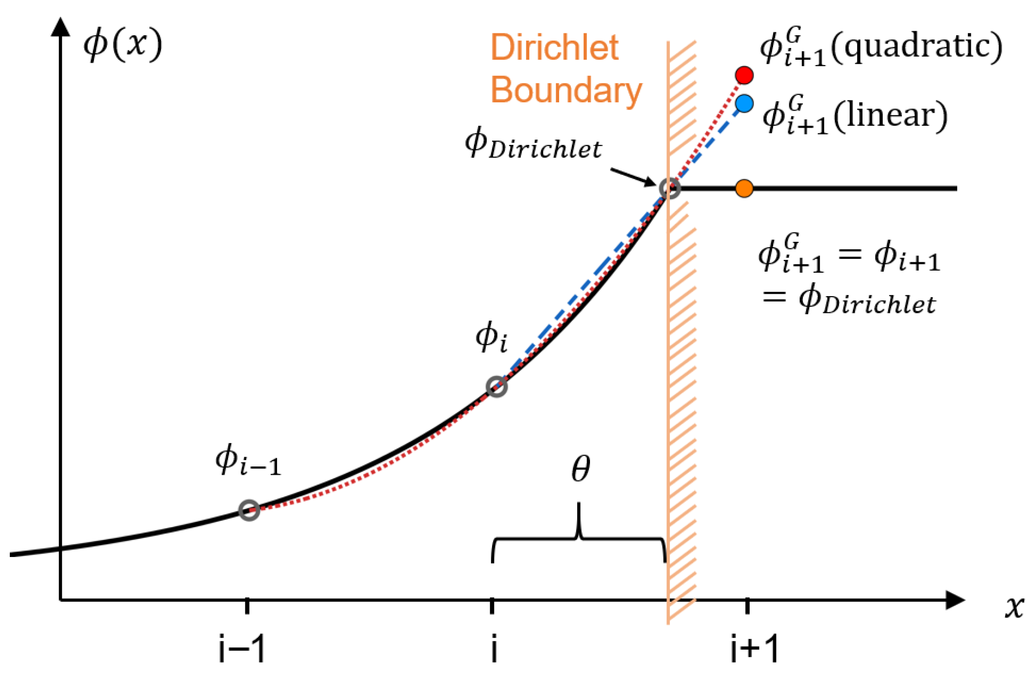
Figure 1. One-dimensional problem illustration with a Dirichlet boundary positioned between nodes.
Computation 14 00013 g001
Figure 2. RHS inaccuracy encountered in PIC simulations illustrated in 1D. The particle marked in red is used to illustrate its cloud size.
Computation 14 00013 g002
Figure 3. Two-dimensional illustration for RHS value treatment for a near-boundary node ( i , j ) .
Computation 14 00013 g003
Figure 4. Comparison of the leading error terms in τ 1 among four scenarios. The circle denotes the point at θ = 0.5 , where the RHS-affected linear and quadratic schemes have the same magnitude of leading truncation error terms.
Computation 14 00013 g004
Figure 5. Comparison of the leading error terms in ξ i L among the four scenarios.
Computation 14 00013 g005
Figure 6. Illustration of a typical near-boundary node in 2D problems that is imperfectly positioned along both axial directions.
Computation 14 00013 g006
Figure 7. The contour of the linear scheme’s leading error term coefficients comparison with/without inaccurate RHS effect across the entire range of θ x and θ y . Panel (a) compares the coefficients of the 2 ϕ / x 2 terms by subtraction, where negative values means RHS-affected linear scheme has lower truncation errors; panel (b) compares the 2 ϕ / y 2 terms; panel (c) combines the results of (a,b), assuming 2 ϕ / x 2 2 ϕ / y 2 .
Computation 14 00013 g007
Figure 8. The contour of leading error term coefficients comparison between the linear and the quadratic scheme under inaccurate RHS effect across all range of θ x and θ y . Panel (a) compares the coefficients of the 2 ϕ / x 2 terms by subtraction, where negative values means RHS-affected linear scheme has lower truncation errors; panel (b) compares the 2 ϕ / y 2 terms; panel (c) combines the results of (a,b), assuming 2 ϕ / x 2 2 ϕ / y 2 .
Computation 14 00013 g008
Figure 9. The numerical errors from solving the 1D Poisson equation with and without the RHS effect by the linear scheme. A total number of 161 nodes were set evenly within the domain [ 0.5 , 0.5 ] , the Dirichlet boundaries were set at ± 0.3156 to give θ L , θ R =0.5.
Computation 14 00013 g009
Figure 10. The numerical errors from solving the 1D Poisson equation with and without the RHS effect by the quadratic scheme. A total number of 161 nodes were set evenly within the domain [ 0.5 , 0.5 ] , the Dirichlet boundaries were set at ± 0.3156 to give θ L , θ R =0.5, the boundary error contributions only plotted for the RHS case.
Computation 14 00013 g010
Figure 11. Comparison between the errors from the RHS-affected linear and quadratic scheme solutions. A total number of 161 nodes were set evenly within the domain [ 0.5 , 0.5 ] , and the Dirichlet boundaries were set at ± 0.3156 to give θ L , θ R = 0.5.
Computation 14 00013 g011
Figure 12. Comparison between δ i values calculated by Equation (8) and those from more accurate integration Equation (7), selected θ values are 0.0, 0.3, 0.5, 0.7, and 1.0. The horizontal dashed lines represent the accurate δ i values calculated by the integral equation, whereas the solid lines represent those calculated by the simpler Equation (8).
Computation 14 00013 g012
Figure 13. The relative RHS sampling errors affected by the partition level and the number of nodes per dimension in the 2D test case. Panel (a) presents the average RHS sampling error of inner nodes; panel (b) depicts the maximum error. The tested partition levels range from 1 to 5, with the data for level 3 highlighted in red. The horizontal dashed line denotes a relative error of 1.0 × 10 4 , serving as a reference.
Computation 14 00013 g013
Figure 14. The relative RHS sampling errors affected by the partition level and the number of nodes per dimension in the 3D test case. Panel (a) presents the average RHS sampling error of inner nodes; panel (b) depicts the maximum error. The tested partition levels range from 1 to 4, with the data for level 3 highlighted in red. The horizontal dashed line denotes a relative error of 1.0 × 10 4 , serving as a reference.
Computation 14 00013 g014
Figure 15. The computational domain for the 2D case with a total 41 × 41 uniformly spaced nodes, the open circles with a cross indicate the near-boundary nodes.
Computation 14 00013 g015
Figure 16. The θ x and θ y values associated with each near-boundary node. Each open circle corresponds to a particular near-boundary node; a total number of 151 × 151 nodes were used on the computational domain.
Computation 14 00013 g016
Figure 17. Contours of the comparison between the RHS-affected linear case and the ordinary linear case in terms of the truncation and numerical errors for all near-boundary nodes, each of which corresponds to a particular ( θ x , θ y ) pair. A total number of 151 × 151 nodes were employed on the computational domain. Panels (a,b) show the comparison of the leading truncation error component associated with ϕ 2 / x 2 and ϕ 2 / y 2 , respectively. Panel (c) compares the overall truncation error magnitude, and panel (d) compares the resulting numerical errors.
Computation 14 00013 g017
Figure 18. Contours of the comparison b of the comparison between the RHS-affected linear case and the RHS-affected quad case in terms of the truncation and numerical errors for all near-boundary nodes, each of which corresponds to a particular θ x and θ y pair. Panels (a,b) show the comparison of the leading truncation error component associated with ϕ 2 / x 2 and ϕ 2 / y 2 , respectively. Panel (c) compares the overall truncation error magnitude, and panel (d) compares the resulting numerical errors.
Computation 14 00013 g018aComputation 14 00013 g018b
Figure 19. The plots of the truncation errors and the final numerical errors at all nodes from solving the 2D Poisson equation by the linear scheme. Panel (a) shows the truncation errors, and panel (b) shows the resulting numerical errors, which were inverted for better comparison.
Computation 14 00013 g019
Figure 20. The plots of the truncation errors and the final numerical errors at all nodes from solving the 2D Poisson equation by the quadratic scheme. Panel (a) shows the truncation errors, and panel (b) shows the resulting numerical errors, which were inverted for better comparison.
Computation 14 00013 g020
Figure 21. Plots of the truncation errors and the final numerical errors at all nodes from solving the 2D Poisson equation by the linear scheme with the inaccurate RHS effect. Panel (a) shows the truncation errors, and panel (b) shows the resulting numerical errors, which were inverted for better comparison.
Computation 14 00013 g021
Figure 22. Plots of the truncation errors and the final numerical errors at all nodes from solving the 2D Poisson equation by the quadratic scheme with the inaccurate RHS effect. Panel (a) shows the truncation errors, which were inverted for better comparison, and panel (b) shows the resulting numerical errors.
Computation 14 00013 g022
Figure 23. Plots of the truncation errors and the final numerical errors at all nodes from solving the 2D Poisson equation by the RHS-affected quadratic scheme, where the RHS values were modified by b i , j = b i , j ¯ / δ i , j ¯ for the near-boundary nodes. Panel (a) shows the truncation errors, and panel (b) shows the resulting numerical errors, which were inverted for better comparison.
Computation 14 00013 g023
Table 1. Numerical errors from solving the 2D case, using accurate RHS values b i , j .
Linear ExtrapolationQuadratic Extrapolation
number
of nodes
L 1 errororder L errororder L 1 errororder L errororder
41 × 418.013 × 10−62.047 × 10−52.3643 × 10−76.7915 × 10−7
81 × 812.097 × 10−61.936.198 × 10−61.725.8779 × 10−82.001.7224 × 10−71.82
161 × 1615.262 × 10−71.991.654 × 10−61.911.1756 × 10−6−4.39.7126 × 10−4−12.5
Table 2. Numerical errors from solving the 2D case, using inaccurate RHS values b i , j ¯ .
Linear ExtrapolationQuadratic Extrapolation
number
of nodes
L 1 errororder L errororder L 1 errororder L errororder
41 × 411.3931 × 10−67.7411 × 10−65.1160 × 10−61.7039 × 10−5
81 × 813.8876 × 10−71.842.8273 × 10−61.451.3768 × 10−61.894.2559 × 10−62.00
151 × 1511.0415 × 10−72.108.4515 × 10−71.923.6962 × 10−72.091.2271 × 10−61.98
Table 3. Numerical errors from solving the varied 2D case, where the RHS values are uniformly distributed as b = 4 .
Accurate RHS bInaccurate RHS b i , j ¯ Modified b i , j ˜ = b i , j ¯ / δ i , j ¯
Number of
Nodes Used
Linear L Quad L Linear L Quad L Linear L Quad L
41 × 415.728 × 10−42.498 × 10−163.499 × 10−46.201 × 10−45.708 × 10−42.498 × 10−16
81 × 811.446 × 10−45.551 × 10−168.386 × 10−51.482 × 10−41.446 × 10−45.551 × 10−16
161 × 1613.803 × 10−51.032 × 10−61.652 × 10−53.603 × 10−53.803 × 10−51.032 × 10⁻⁶
Table 4. Two-dimensional test case with nonuniform b i , j —the numerical error results obtained using different treatments of RHS values.
Accurate RHS b i , j Inaccurate RHS b i , j ¯ Modified b i , j ˜ = b i , j ¯ / δ i , j ¯
Number
of Nodes
Linear L Quad L Linear L Quad L Linear L Quad L
41 × 412.047 × 10−56.792 × 10−77.741 × 10−61.704 × 10−51.957 × 10−58.614 × 10−7
81 × 816.198 × 10−61.722 × 10−72.827 × 10−64.256 × 10−66.039 × 10−61.652 × 10−7
151 × 1511.7752 × 10−64.9798 × 10−88.4515 × 10−71.2271 × 10−61.7526 × 10−64.8523 × 10⁻⁸
Table 5. Three-dimensional test case with nonuniform b i , j , k —the numerical error results obtained using different treatments of RHS values.
Accurate RHS b i , j , k Inaccurate RHS b i , j , k ¯ Modified b i , j , k ˜ = b i , j , k ¯ / δ i , j , k ¯
Number
of Nodes
Linear L Quad L Linear L Quad L Linear L Quad L
26 3 2.007 × 10−41.113 × 10−57.294 × 10−51.768 × 10−41.880 × 10−46.039 × 10−6
51 3 4.939 × 10−52.348 × 10−62.076 × 10−54.621 × 10−54.779 × 10−51.747 × 10−6
101 3 1.284 × 10−55.281 × 10−75.724 × 10−61.187 × 10−51.263 × 10−54.599 × 10−7
Table 6. Computational times for the 3D test cases.
Accurate RHS b i , j , k Inaccurate RHS b i , j , k ¯ Modified b i , j , k ˜ = b i , j , k ¯ / δ i , j , k ¯
Number
of Nodes
Linear Quad Linear Quad Linear Quad
26 3 7.311× 10−31.158 × 10−25.538 × 10−25.955 × 10−29.972 × 10−21.057 × 10−1
51 3 5.092 × 10−21.230 × 10−12.576 × 10−13.219 × 10−14.465 × 10−15.137 × 10−1
101 3 1.0904.6471.8855.4202.6576.205
Disclaimer/Publisher’s Note: The statements, opinions and data contained in all publications are solely those of the individual author(s) and contributor(s) and not of MDPI and/or the editor(s). MDPI and/or the editor(s) disclaim responsibility for any injury to people or property resulting from any ideas, methods, instructions or products referred to in the content.