Abstract
Accurate trajectory control during atmospheric entry is critical for the success of Mars landing missions, where strong non-linearities and uncertain dynamics pose significant challenges to conventional control strategies. This study develops a computational framework that integrates fuzzy parameter-varying models with Lyapunov-based analysis to achieve robust trajectory stabilization of Mars entry vehicles. The non-linear longitudinal dynamics are reformulated via sector-bounded approximation into a Takagi–Sugeno fuzzy parameter-varying model, enabling systematic gain-scheduled controller synthesis. To reduce the conservatism typically associated with quadratic Lyapunov functions, a fuzzy Lyapunov function approach is adopted, in conjunction with the Full-Block S-procedure, to derive less restrictive stability conditions expressed as linear matrix inequalities. Based on this formulation, several controllers are designed to accommodate the variations in atmospheric density and flight conditions. The proposed methodology is validated through numerical simulations, including Monte Carlo dispersion and parametric sensitivity analyses. The results demonstrate improved stability, faster convergence, and enhanced robustness compared to existing fuzzy control schemes. Overall, this work contributes a systematic and less conservative control design methodology for aerospace applications operating under severe non-linearities and uncertainties.
1. Introduction
Accurate route monitoring during a vehicle’s penetration of Mars’ atmosphere remains a computationally intensive challenge due to the highly non-linear dynamics, time-varying environmental conditions, and modeling uncertainties inherent to planetary descent. Developing robust control algorithms for such systems requires not only precise dynamic modeling but also computationally tractable methods for controller synthesis and validation. In this context, computational control strategies based on fuzzy system modeling and convex optimization offer a promising pathway for managing uncertainty and non-linearity in real-time. This study leverages fuzzy parameter-varying (FPV) models and Lyapunov-based analysis to construct a control framework that is both mathematically rigorous and suitable for numerical implementation in aerospace guidance systems.
Since the success of the first Mars probe mission, spacefaring nations have intensified their efforts to develop high-precision landing technologies for Martian exploration vehicles [1,2,3]. These advancements are critical to enabling more sophisticated and targeted scientific investigations on the Martian surface. However, achieving accurate landings remains a significant challenge, primarily due to various sources of uncertainty, particularly during the atmospheric entry phase. The Martian atmosphere is characterized by its harsh climate, pronounced temporal variability, and non-linear dynamics [4,5,6], all of which complicate precise descent and landing control. In this context, the application of fuzzy parameter-varying control systems presents a practical and computationally efficient approach to enhancing trajectory tracking performance and improving the robustness of guidance and control strategies under such uncertain and dynamic conditions.
The Takagi–Sugeno (T–S) fuzzy framework has become a cornerstone for modeling and controlling time-varying, non-linear systems due to its strong approximation capabilities. In 2007, Tanaka et al. [7] introduced a descriptor-system formulation for fuzzy control that leverages fuzzy Lyapunov functions to reduce the number of linear matrix inequality (LMI) conditions and thus the computational burden, which is required for stability analysis. By tailoring both the controller structure and the Lyapunov function, their approach explicitly accounts for the switching speed of individual linear subsystems via lower bounds on the time-derivative of the membership functions, yielding less conservative linear matrix inequalities (LMIs).
Building on this, Li, Zhou, and Xu [8] (2008) derived new sufficient conditions for stability that dispense with any bounds on the membership-function derivatives. Their fuzzy Lyapunov-based criteria enlarge the certifiable stability region compared with earlier methods. In 2013, Lam and Lauber [9] further extended this line of work by analyzing closed-loop stability for T–S fuzzy systems under fuzzy-controller interconnection, again employing fuzzy Lyapunov functions to rigorously characterize system behavior. In 2016, Liu et al. [10] addressed the conservatism and computational complexity inherent in existing relaxation techniques by introducing a linear fractional transformation (LFT) mechanism combined with the full-block S-procedure. This novel relaxation method significantly reduces conservatism in both analysis and dynamic output-feedback controller synthesis for continuous-time T–S fuzzy systems.
More recently, Zhang et al. [11] (2018) proposed a fuzzy parameter-varying system that unifies the advantages of T–S fuzzy models and linear parameter-varying (LPV) systems. They provided LMI-based conditions guaranteeing global asymptotic stability and synthesized a state-feedback law that stabilizes the closed-loop fuzzy parameter-varying plant. In 2024, two significant advances were reported. First, Tang [12] developed a finite-time stabilization method for delayed, uncertain T–S fuzzy systems under intermittent control. By formulating a new finite-time stability lemma, he obtained less-conservative LMI conditions and overcame challenges in assessing performance when control is applied intermittently. Second, Liu et al. [13] introduced a secure, fault-tolerant control (FTC) architecture for T–S fuzzy cyber–physical systems (CPSs) operating in hostile network environments. Their multi-observer scheme decouples and suppresses sparse sensor attacks, system faults, and unknown disturbances, demonstrating effectiveness in an autonomous-vehicle control scenario. Together, these developments illustrate a clear trajectory toward ever more efficient, less conservative, and more resilient fuzzy control designs, which are critical capabilities for modern applications ranging from autonomous vehicles to aerospace systems.
These developments represent significant progress in the application of fuzzy Lyapunov functions within fuzzy theory [14,15,16]. This modeling approach effectively mitigates the rapid increase in the number of fuzzy rules typically encountered when applying the traditional Takagi–Sugeno (T–S) fuzzy framework to time-varying systems. The fuzzy Lyapunov function is then employed to perform stability analysis and facilitate the design of parameter-dependent controllers. Compared to conventional quadratic Lyapunov functions, this approach offers improved accuracy in capturing the dynamic behavior of the system. Furthermore, the successful integration of non-linear parameter-varying theory [17] into the trajectory control strategy during the entry phase of the Mars probe [18,19,20] enhances the robustness and precision of trajectory tracking under highly non-linear and time-varying atmospheric conditions.
This work makes a substantial contribution to the computational modeling and control of non-linear aerospace systems through
- The development of a fuzzy parameter-varying framework tailored for Mars atmospheric entry, providing a novel approach to the computational modeling and control of non-linear aerospace systems.
- An accurate representation of complex aerodynamic interactions during entry through a sector-bounded approximation and fuzzy rule partitioning, enabling a tractable description of non-linear dynamics.
- An introduction of a refined stability analysis that departs from conventional quadratic Lyapunov functions by employing fuzzy Lyapunov function synthesis in combination with the Full-Block S-procedure.
- A reduction in conservatism in robust control design and the facilitation of gain-scheduled controller construction using linear matrix inequality (LMI) optimization.
The entire framework is validated through numerical simulations, including parametric sensitivity analysis and Monte Carlo dispersion tests, demonstrating both the computational efficiency and practical robustness of the proposed approach. By bridging theoretical control design with simulation-driven validation, this study advances computational techniques for stability analysis and control synthesis in non-linear, time-varying environments relevant to critical aerospace applications.
The paper is structured as follows: Section 2 presents the formulation of a longitudinal fuzzy parameter-varying model for the Mars entry system. Section 3 provides stability analysis of the system. Section 4 details the design methodologies for parameter-dependent state-feedback and dynamic output-feedback gain-scheduled controllers. Section 5 reports the simulation results that validate the effectiveness of the proposed control strategies. Finally, Section 6 concludes the paper with a summary of key findings and main contributions.
2. Mathematical Modeling
We first introduce the following non-dimensional longitudinal models [20,21,22,23] for the entry phase of Mars exploration probes:
Here, denotes the radial distance between the Mars probe and the center of Mars. The variable represents the velocity of the probe, and is the flight path angle (in radians), where . The dimensionless drag and lift forces are defined as
where and are the drag and lift coefficients, respectively; s is the reference area; is the atmospheric density; m is the mass of the probe; and g is the gravitational acceleration. Some other symbols in Table 1.

Table 1.
The symbols in this article.
In [24], a novel non-linear modeling approach was introduced, integrating the strengths of both the Takagi–Sugeno (T–S) fuzzy system and the linear parameter-varying (LPV) framework. To facilitate controller design for the Mars entry system, the longitudinal non-linear dynamics of the probe must be reformulated into a fuzzy parameter-varying model. This transformation is carried out in two main steps. First, the original non-linear system is approximated by a linear representation using sector non-linearity techniques. Subsequently, fuzzy partitioning is applied to capture the system’s varying behavior across different operating conditions. Following these steps and choosing the atmosphere density of Mars as a time-varying parameter yield the following FPV system [11,20,25]:
where y denotes measurement output, u denotes control input signal, , , , and .
The fuzzy rules of Model (2) are given as follows: If , and , then
where . are fuzzy sets, with . The coefficient matrices have the following structures:
Here, x represents the state vector (radial distance, velocity, and flight path angle); u is the control input; y is the measurement output; and is the Martian atmospheric density (a time-varying parameter). The model uses fuzzy rules to partition the system’s behavior across different operating conditions, with as membership functions. The matrices are defined based on aerodynamic forces and system parameters, enabling systematic controller design and stability analysis using fuzzy Lyapunov functions. This approach mitigates the conservatism of traditional quadratic Lyapunov methods and enhances trajectory tracking robustness under uncertain atmospheric conditions.
3. System Stability Analysis
The Martian atmospheric entry involves extreme non-linear dynamics and time-varying uncertainties (e.g., fluctuating atmospheric density), where unstable model solutions would lead to uncontrolled trajectory deviations. For instance, an unstable system could cause the entry vehicle to crash prematurely, escape the atmosphere, or experience structural failures due to unbounded oscillations. However, exclusive reliance on quadratic Lyapunov functions often introduces excessive conservatism, limiting the achievable performance and robustness of the system [26,27]. To address this limitation, this section adopts a fuzzy Lyapunov function to conduct a less conservative stability analysis.
Let us consider the open-loop system, as illustrated in (3), under the condition of zero control inputs. Employing the fuzzy Lyapunov function methodology, this subsection undertakes a comprehensive stability analysis of the fuzzy parameter-varying system. The analysis is accomplished by virtue of the Full-Block S-procedure, as expounded in [28].
The stability analysis of the fuzzy parameter-varying model is fundamental for ensuring reliable trajectory control during Mars atmospheric entry. Traditional approaches relying on quadratic Lyapunov functions often introduce excessive conservatism, limiting the controller’s robustness in handling time-varying uncertainties. To overcome this, we propose a novel stability theorem based on fuzzy Lyapunov function synthesis, which explicitly accounts for the system’s parameter variations and reduces conservatism under linear matrix inequality (LMI) conditions. The key motivation for developing Theorem 1 stems from the need to address two critical limitations of conventional stability analysis: Conservatism in quadratic Lyapunov functions: Quadratic Lyapunov functions assume fixed positive definite matrices, which fail to capture the dynamic behavior of parameter-varying systems accurately. Handling time-varying parameters: The Martian atmospheric density and flight dynamics evolve rapidly, requiring a stability framework that adapts to these variations in real time.
The following Lemma (Lemma 1) [20] is established based on fuzzy system theory.
Lemma 1.
Assume . If there exist a positive definite matrix of appropriate dimension, , and two multipliers, , , satisfying flowing LMIs
for and some , where
with and , then System (3) is asymptotically stable.
The Lemma is inherently linked to the fuzzy rules through the fuzzy parameter-varying system structure, where each rule defines a local linear subsystem corresponding to specific operating conditions. 1. The fuzzy rules partition the non-linear dynamics into linear submodels, and the theorem’s stability conditions ensure that the convex combination of these submodels (weighted by membership functions ) remains asymptotically stable. Specifically, the theorem leverages the fuzzy rules to construct a Lyapunov function that adapts to parameter variations, with each in . To ensure the theorem’s conditions hold, one can adopt two complementary approaches: (1) Convex Optimization Check: Formulate LMIs (5)–(8) as a convex programming problem that is solvable via tools like MATLAB’s (version 2023a) LMI Control Toolbox, which checks for the existence of , F, and multipliers , . (2) Vertex Analysis: Since (a convex set of atmospheric densities), verify stability at the set’s vertices , as convex combinations of stable vertices ensure global stability. This approach reduces complexity by leveraging the vertex property of convex systems, ensuring the conditions hold for all within .
4. Controller Design
A substantial body of research on T–S fuzzy systems has been conducted using the quadratic Lyapunov function as the foundation for stability analysis. However, when the controlled system involves a large number of time-varying parameters, it may become difficult or even impossible to identify a constant positive definite matrix that guarantees closed-loop stability in the Lyapunov sense. To overcome this limitation, this section presents the design of both a state-feedback gain-scheduling controller and a dynamic output-feedback gain-scheduling controller. The controller design is carried out based on the stability conditions derived from the fuzzy Lyapunov function framework, offering a more flexible and less conservative approach to ensuring system stability under complex, time-varying conditions.
4.1. State-Feedback Controller
The fuzzy parameter-varying system is considered as follows:
where denotes the evaluation output, interference input, and control input signal, respectively. The coefficient matrices depend on , satisfying the following requirements:
- .
Consider the following parameter-dependent state-feedback controller:
Substitute (9) into (8). The following result could be obtained:
The state-feedback gain-scheduling controller is developed by employing the Full-Block S-procedure in conjunction with the bounded real Lemma [10]. The formal statement of the corresponding theorem is provided below.
Theorem 1.
Assume the bound of is . γ and are positive. If there exist a positive definite matrix of appropriate dimension, , F, and two multipliers , for some satisfying
where ,
 then the following states feedback controller can control the following system (System (8)):
for any , and the system gain of (8) is less than γ.
then the following states feedback controller can control the following system (System (8)):
for any , and the system gain of (8) is less than γ.
then the following states feedback controller can control the following system (System (8)):State-feedback controllers bring unique strengths to control design. They let you fine-tune dynamic setting time, damping, and overshoot by placing poles precisely, using all state info to resist disturbances. The design simplifies with tools like LQR balancing performance and effort, and they keep complex systems in sync, avoiding cross-talk.
4.2. Dynamical Output-Feedback Controller Design
Compared to the state-feedback controller, the output-feedback controller is more suitable for applications. Consider the following FPV system:
Assume the dynamical output feedback controller has the following form:
where denotes the controller’s state, and the coefficient matrices of controller are all unknown. We will have the following theorem.
Theorem 2.
Assume . If there exist matrices of appropriate dimension, namely , , , , and positive matrices, such as , , and , for some satisfying
with , , then System (18) is stabilized by the controller (Equation (19)), and the coefficient matrix of the controller is as follows:
then System (18) is stabilized by the controller (Equation (19)), and the coefficient matrix of the controller is as follows:4.3. Remarks
Although state-feedback controllers for aircraft trajectory tracking offer substantially lower computational complexity compared to output-feedback counterparts, their practical implementation is often constrained. In aircraft systems, a full-state measurement is rarely feasible: certain states cannot be directly sensed, and full-state monitoring requires high-precision sensors, which increase both cost and weight [29]. Consequently, state-estimation techniques [30] or dynamic output-feedback control become essential to ensure stable and accurate trajectory tracking. In this regard, several studies have demonstrated the effectiveness of output-feedback approaches under practical constraints. For instance, ref. [31] proposed an dynamic output-feedback controller for aircraft trajectory tracking under actuator faults, employing a discrete-time model that incorporates network-induced delays. Its design, based on linear matrix inequality (LMI) optimization, achieved reliable tracking performance using only measurable variables and provided fault tolerance information. Building on this, ref. [32] validated the applicability of this strategy to non-linear aircraft models, showing its ability to mitigate wind gust disturbances and compensate for partial actuator failures. Collectively, these contributions confirm the practical value of dynamic output-feedback control when state feedback is limited by sensing constraints. In this study, we adopt state feedback under the assumption of ideal measurement conditions as a first step toward establishing our framework. Nevertheless, future work could extend the proposed approach to dynamic output-feedback control, thereby improving its robustness and applicability to real-world aircraft scenarios involving sensor limitations, network delays, or actuator faults.
5. Numerical Illustration
To enhance the scientific rigor of this study, this section presents a comparative analysis of the system’s performance with and without the proposed controller. The evaluation is conducted through numerical simulations implemented in MATLAB.
System parameters are selected as follows: [20] and . The corresponding matrices of System 8 can be readily obtained through straightforward calculations, which are provided in Appendix A for reference. Based on Theorem 1, the simulation results are obtained using MATLAB, as illustrated below. We simulate System (8) without the support of Controller (17), and the results are displayed in Figure 1. The figures show that System (8) is unstable in the absence of Controller (17).
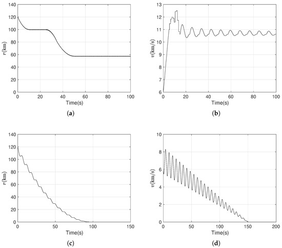
Next, based on Theorem 1, we obtain the state-feedback controller (Controller (17)) with and , where . From Inequalities (11)∼(16), we can obtain controller matrices. The result depicted in Figure 1 is obtained. The analysis of the figures reveals that state r and v are zeros, indicating the asymptotic stability of System (8) under Controller (17). To verify the efficiency of the method we proposed, we select the following parameters for the system matrix:
It is not difficult to infer from Figure 2a that the stabilization region of this method (Theorem 1) is the largest. It has fewer decision variables, fewer LMIs, and requires less computation time (see Table 2).
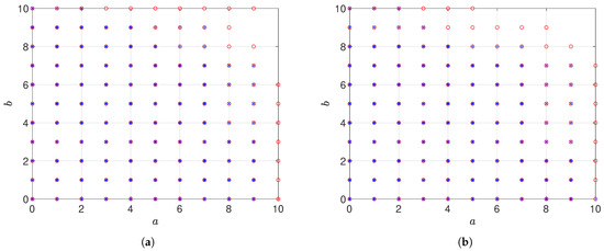
Figure 2.
Stabilization region; legend: o → our work; ×→ ref. [11]; +→ ref. [10] (a) Stabilization region of Theorem 1. (b) Stabilization region of Theorem 2.
Table 2.
Comparison of computational complexity for state-feedback controllers.
Consistent with the preceding analysis, the same parameter data are employed for (18). The coefficient matrices of (18) are derivable via straightforward computations. By substituting the results obtained from Equations (20) to (27) into Controller (19) and conducting simulations on System (18), the outcomes depicted in Figure 3 are generated. The analysis of the graphical results indicates that the states r and v asymptotically converge to 0 at 62 s, thereby validating the efficacy of the designed dynamic output-feedback controller (Controller (19)) in stabilizing System (18). It is not difficult to find from Figure 2b that the stabilization region of this method (Theorem 1) is the largest. It has fewer decision variables, fewer LMIs, and requires less computation time (see Table 3). Figure 4 shows that this output-feedback controller designed by Theorem 2 enables the system to have good tracking capability.
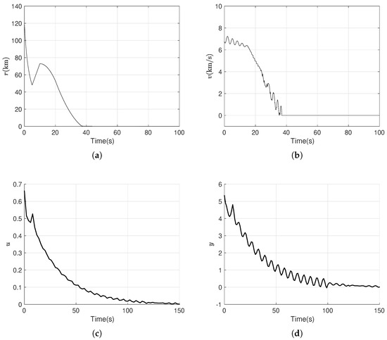
Table 3.
Comparison of computational complexity for output-feedback controllers.
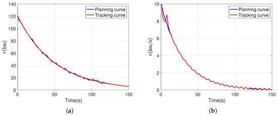
Figure 4.
(a) Tracking curve of r. (b) Tracking curve of v.
To validate the superiority of the designed controller, we simulate System (18) with the Parallel Distributed Compensation (PDC) controller which is designed with the method given in [11], and then compare it with the full state-feedback and the dynamical output-feedback gain-scheduling controllers. The simulation results are displayed in Figure 3. As can be seen from Figure 1, Figure 2 and Figure 3, the state-feedback controller and the dynamic output-feedback controller can make the system gradually stabilize in a shorter amount of time, which indicates that their control effects are better than those of the PDC controller. Furthermore, the analysis of the figures indicates that the states r and v of the Mars probe with the state-feedback controller and the dynamic output-feedback controller asymptotically converge to zero at about 150 s and 100 s, respectively. Therefore, the dynamic output-feedback controller is better than the state-feedback controller in terms of the time needed to gradually stabilize the system.
6. Conclusions
This paper develops a computationally efficient fuzzy control framework for robust trajectory tracking of Mars entry vehicles under non-linear and time-varying conditions. By reformulating the non-linear entry dynamics into a fuzzy parameter-varying system via sector non-linearity techniques, the proposed method facilitates systematic controller synthesis using linear matrix inequality (LMI)-based optimization. The core contribution lies in the construction of a fuzzy Lyapunov function framework that enables less conservative stability analysis compared to traditional quadratic approaches while accommodating time-varying parameters such as atmospheric density.
Two types of gain-scheduled controllers, state-feedback and dynamic output-feedback controllers, are designed using the Full-Block S-procedure to ensure stability and performance under parametric uncertainties. The computational tractability of the control design process is maintained through convex optimization formulations, making the approach scalable for high-dimensional fuzzy systems. Extensive numerical simulations, including sensitivity analysis and Monte Carlo tests, confirm the effectiveness of the proposed controllers in achieving faster convergence and higher robustness compared to conventional methods, such as Parallel Distributed Compensation (PDC).
The computational techniques introduced in this work contribute to advancing non-linear control synthesis for aerospace applications and are readily extensible to other high-stakes systems with uncertainty and non-linearity. Future work will focus on extending the framework to coupled translational–rotational entry dynamics, integrating real-time adaptive estimation, and leveraging high-performance computing for onboard trajectory optimization under uncertainty.
Author Contributions
Conceptualization, H.Z. and N.M.; methodology, H.Z.; software, H.Z. and and N.M.; validation, H.Z.; formal analysis, S.X. investigation, H.Z.; resources, S.X.; writing—original draft preparation, H.Z.; writing—review and editing, S.X. All authors have read and agreed to the published version of the manuscript.
Funding
This research received no external funding.
Data Availability Statement
The original contributions presented in this study are included in the article. Further inquiries can be directed to the corresponding author.
Acknowledgments
The authors would like to thank the anonymous referees and editors for their valuable comments and constructive suggestions.
Conflicts of Interest
The authors declare no conflicts of interest.
Correction Statement
This article has been republished with a minor correction to the Data Availability Statement. This change does not affect the scientific content of the article.
Appendix A
The proof of Lemma 1 is shown below.
Proof.
Take as the fuzzy Lyapunov candidate function and compute its derivative along the trajectory of System (3).
For , by constraining , we have the following form:
Due to , is between and ; here, , while . Then,
where . Equation (A3) is equal to
From Theorem 2.1 [28], there exists a multiplier , such that
It is clear that
where
Then, Inequality (A5) can be rewritten as the following form:
Knowing that and , we can write inequalities (A6) and (A10) in the following form using convex optimization theory [10]:
□
The proof of Theorem 1 is shown below.
Proof.
Take as the fuzzy Lyapunov candidate function and a controller with the form of . Compute its derivative along the trajectory of System (10).
According to the convex optimization theory, the inequality is guaranteed by
for ; here,
It is obvious that
Thus, it is equivalent to the following result:
According to the Schur Complement [10] of a matrix, (A18) holds if and only if the following matrix inequality holds:
Equation (A19) can be expressed as the following form:
Multiply the matrix on the left and right sides at the same time to obtain the following result:
Equation (A21) has the following form:
Equation (A21) can be written in the following form of expression:
Here, and satisfies
where ,
and satisfies
where ,
and satisfies Equation (A22) is no longer dependent on h after using the Full-Block S-procedure Theorem, and all coupling terms of h and are eliminated successfully. But the quadratic terms about still exist, so we use the Full Block S-procedure Theorem again. in (A23) can be decomposed into the following form:
where Thus,
Equation (A23) can be written in the following form of expression:
where . It is clear that Equations (A15), (A24), (A25), (A28), (A29), and (A30) guarantee that System (8) can be controlled by the state-feedback gain-scheduling controller (Controller (9)). □
Thus,
Equation (A23) can be written in the following form of expression:
where . It is clear that Equations (A15), (A24), (A25), (A28), (A29), and (A30) guarantee that System (8) can be controlled by the state-feedback gain-scheduling controller (Controller (9)). □
Thus,The proof of Theorem 2 is shown below.
Proof.
We define that , , , and . We have
where .
Denote . can be decomposed into the following form:
Combine System (18) and Controller (19); then the following closed-loop system is obtained:
It is clear that
Equation (A32) can be expressed as the following form:
The next work is to transform Expression (A33) into a linear matrix inequality with respect to . Suppose that the positive definite matrix and its inverse matrix have the following block form: . Because , the following equations hold:
By introducing nonsingular contract transformation and multiplying the matrix and on the left and right sides of (A33) at the same time, we obtain the following result:
where
So, (A33) can be expressed as the following form:
where
Equation (A36) is linear matrix inequality about and . As long as and are obtained, the gain matrix of the controller can be calculated. But there are still coupling terms about H and in (A36). In order to facilitate the subsequent derivation, we assume the following: Matrix is quadratic with respect to H and . Matrix and matrix are bilinear with respect to H and , and matrix is a constant matrix. Since these membership functions satisfy , these matrices have the following form:
- , where . As for , we have
It satisfies
Since Inequality (A40) is convex with respect to the variables and , Inequality (A40) is equivalent to (23) and (25). □
References
- Ye, P.; Sun, Z.; Rao, Z.; Meng, L. Mission overview and key technologies of the first Mars probe of China. Sci.-China-Technol. Sci. 2017, 60, 649–657. [Google Scholar] [CrossRef]
- Goossens, S.; Sabaka, T.; Rao, Z. Probing Lateral Density Variations in the Crust from Gravity and Topography: Applications to the Moon and Mars. Planet. Sci. J. 2025, 6, 71. [Google Scholar] [CrossRef]
- Guinard, A.; Fienga, A.; Mémin, A.; Ganino, C. Coupled tidal tomography and thermal constraints for probing Mars viscosity profile. Icarus 2025, 425, 116318. [Google Scholar] [CrossRef]
- Zhang, W.; Xu, B.; Li, T.; Zhang, H.; Xiang, C.; Fan, W.; Zhao, Z. Analysis of Aerodynamic Characteristics of Propeller Systems Based on Martian Atmospheric Environment. Drones 2023, 7, 397. [Google Scholar] [CrossRef]
- Zhao, Z.; Jing, Q.; Zhong, W. Comparison of the influence of Martian and Earth’s atmospheric environments on terahertz band electromagnetic waves. Int. J. Commun. Syst. 2021, 34, e4894. [Google Scholar]
- Zhang, J.; Guo, J.; Dobynde, M.; Wang, Y.; Wimmer-Schweingruber, R. From the Top of Martian Olympus to Deep Craters and Beneath: Mars Radiation Environment Under Different Atmospheric and Regolith Depths. J. Geophys.-Res.-Planets 2022, 127, e2021JE007157. [Google Scholar] [CrossRef]
- Tanaka, K.; Ohtake, H.; Wang, H.O. A Descriptor System Approach to Fuzzy Control System Design via Fuzzy Lyapunov Functions. IEEE Trans. Fuzzy Syst. 2007, 15, 333–341. [Google Scholar] [CrossRef]
- Li, J.; Zhou, S.; Xu, S. Fuzzy Control System Design via Fuzzy Lyapunov Functions. IEEE Trans. Syst. Man, Cybern. Part B (Cybern.) 2008, 38, 1657–1661. [Google Scholar] [CrossRef]
- Lam, H.K.; Lauber, J. Membership-function-dependent stability analysis of fuzzy-model- based control systems using fuzzy Lyapunov functions. Inf. Sci. 2013, 232, 253–266. [Google Scholar] [CrossRef]
- Liu, Y.; Wu, F.; Ban, X. Dynamic output feedback control for continuous-time T-S fuzzy systems using fuzzy Lyapunov functions. IEEE Trans. Fuzzy Syst. 2016, 232, 1155–1167. [Google Scholar] [CrossRef]
- Zhang, H.; Ban, X.; Wu, F. Stability Analysis and Controller Design for a Novel Nonlinear System: Fuzzy Parameter Varying System. J. Intell. Fuzzy Syst. 2018, 34, 4387–4395. [Google Scholar] [CrossRef]
- Tang, R.; Yang, X.; Xiang, Z.; Qing, L. Finite-Time L2 Stabilization of Uncertain Delayed T-S Fuzzy Systems via Intermittent Control. IEEE Trans. Fuzzy Syst. 2024, 32, 116–125. [Google Scholar] [CrossRef]
- Liu, Q.; Long, X.; Li, T.; Chen, C. Attack Resilient Fault Tolerant Control for T-S Fuzzy Cyber-Physical Systems. IEEE Trans. Fuzzy Syst. 2024, 32, 2017–2028. [Google Scholar] [CrossRef]
- Collins, E. Fuzzy Control Systems Design and Analysis: A Linear Matrix Inequality Approach. Automatica 2003, 39, 2011–2013. [Google Scholar] [CrossRef]
- Viadero-Monasterio, F.; Nguyen, A.; Lauber, J.; Boada, M.; Boada, B. Event-Triggered Robust Path Tracking Control Considering Roll Stability Under Network-Induced Delays for Autonomous Vehicles. IEEE Trans. Intell. Transp. Syst. 2023, 24, 14743–14756. [Google Scholar] [CrossRef]
- Viadero-Monasterio., F.; Melendez-Useros, M.; Zhang, N.; Zhang, H.; Boada, B.; Boada, M. Motion Planning and Robust Output-Feedback Trajectory Tracking Control for Multiple Intelligent and Connected Vehicles in Unsignalized Intersections. IEEE Trans. Veh. Technol. 2025, 1–13. [Google Scholar] [CrossRef]
- Li, S.; Jiang, X. Review and Prospect of Guidance and Control for Mars Atmospheric Entry. Prog. Aerosp. Sci. 2014, 69, 40–57. [Google Scholar] [CrossRef]
- Tolson, R.; Willcockson, W.; Desai, P.; Thomas, P. Anomalistic Disturbance Torques During the Entry Phase of the Mars Exploration Rover Missions:A Telemetry and Mars-Surface Investigation. Prog. Aerosp. Sci. 2014, 125, 507. [Google Scholar]
- Xu, H.; Cui, H.; Tian, Y. Comparison of Two Robust Optimal Trajectory Design Methods for Mars Entry. ICIC Express Lett. 2015, 9, 2437–2443. [Google Scholar]
- Huang, Q.; Yang, C.; Zeng, Z.; Ye, Y.; Zhang, H. Trajectory Control of Mars Probe Based on Fuzzy Lyapunov Function. In Proceedings of the 2023 2nd Conference on Fully Actuated System Theory and Applications, Qingdao, China, 14–16 July 2023; pp. 1097–1102. [Google Scholar]
- Braun, R.; Manning, R. Mars Exploration Entry Descent and Landing Challenges. J. Spacecr. Rocket. 2007, 44, 310–323. [Google Scholar] [CrossRef]
- Huang, Y.; Li, H.; Zhang, J.; Du, X. Mars Atmospheric Entry Guidance Design by Sliding Mode Disturbance Observer-Based Control. Procedia Eng. 2015, 99, 1062–1075. [Google Scholar] [CrossRef][Green Version]
- Putnam, Z.; Braun, R. Precision Landing at Mars Using Discrete-Event Drag Modulation. J. Spacecr. Rocket. 2013, 51, 128–138. [Google Scholar] [CrossRef]
- Scherer, C. LPV Control and Full Block Multipliers. Automatica 2001, 37, 361–375. [Google Scholar] [CrossRef]
- Aubry, P.; Marrez, J.; Valibouze, A. Computing Real Solutions of Fuzzy Polynomial Systems. Fuzzy Sets Syst. 2020, 399, 55–76. [Google Scholar] [CrossRef]
- Li, Y.; Jian, C.; Su, H. Robust Memoryless H∞ Controller Design for Linear Time-Delay Systems with Norm-Bounded Time-Varying Uncertainty. Automatica 1996, 32, 1759–1762. [Google Scholar]
- Choi, H.; Chung, H. Memoryless H∞ Controller Design for Linear Systems with Delayed State and Control. Automatica 1995, 31, 917–919. [Google Scholar] [CrossRef]
- Pasquale, G.; Sturz, Y.; Valcher, M.; Smith, R. Extended Full Block S-Procedure for Distributed Control of Interconnected Systems. In Proceedings of the 2020 59th IEEE Conference on Decision and Control (CDC), Jeju, Republic of Korea, 14–18 December 2020; Volume 31, pp. 5628–5633. [Google Scholar]
- Ye, X.; Song, F.; Zhang, Z.; Zhang, R.; Zeng, Q. Semi-Aerodynamic Model-Aided Invariant Kalman Filtering for UAV Full-State Estimation. IEEE Sensors J. 2024, 24, 25920–25939. [Google Scholar]
- Wang, H.; Farid, Y.; Wang, L.; Garone, E.; Preumont, A. Hovering Flight of a Robotic Hummingbird: Dynamic Observer and Flight Tests. Actuators 2024, 13, 91. [Google Scholar] [CrossRef]
- Viadero-Monasterio, F.; Boada, B.; Boada, M.; Diaz, V. H∞ dynamic output feedback control for a networked control active suspension system under actuator faults. Mech. Syst. Signal Process. 2022, 162, 108050. [Google Scholar] [CrossRef]
- Li, Z.; Wang, X.; Guo, H.; Xi, L.; Liu, G.; Li, Y.; Hua, C. Distributed Output Feedback Prescribed Performance Control for High-Order Nonlinear Multi-Agent Systems. IEEE Trans. Autom. Sci. Eng. 2025, 22, 12730–12740. [Google Scholar] [CrossRef]


Disclaimer/Publisher’s Note: The statements, opinions and data contained in all publications are solely those of the individual author(s) and contributor(s) and not of MDPI and/or the editor(s). MDPI and/or the editor(s) disclaim responsibility for any injury to people or property resulting from any ideas, methods, instructions or products referred to in the content. |
© 2025 by the authors. Licensee MDPI, Basel, Switzerland. This article is an open access article distributed under the terms and conditions of the Creative Commons Attribution (CC BY) license (https://creativecommons.org/licenses/by/4.0/).