Abstract
In this paper, we propose the MUSWENO scheme, a novel mapped weighted essentially non-oscillatory (WENO) method that employs unequal-sized stencils, for solving nonlinear degenerate parabolic equations. The new mapping function and nonlinear weights are proposed to reduce the difference between the linear weights and nonlinear weights. Smaller numerical errors and fifth-order accuracy are obtained. Compared with traditional WENO schemes, this new scheme offers the advantage that linear weights can be any positive numbers on the condition that their summation is one, eliminating the need to handle cases with negative linear weights. Another advantage is that we can reconstruct a polynomial over the large stencil, while many classical high-order WENO reconstructions only reconstruct the values at the boundary points or discrete quadrature points. Extensive examples have verified the good representations of this scheme.
MSC:
65M06
1. Introduction
In this paper, a new type mapped unequal-sized weighted essentially non-oscillatory (MUSWENO) scheme is proposed for solving the nonlinear degenerate parabolic equation. The study of nonlinear degenerate parabolic equations dates back to the early 20th century. With the advancement of mathematics and physics, the significance of such equations in describing natural phenomena and engineering problems has become increasingly prominent. Nonlinear degenerate parabolic equations, featuring solution-dependent diffusion coefficients that vanish at critical states, are vital across multiple disciplines. They model porous media flow in fluid mechanics, capturing saturation-dependent permeability and generating finite propagation speeds with sharp wetting fronts. These equations describe heat conduction in materials with temperature-sensitive thermal conductivity, potentially exhibiting finite thermal wave speeds. In phase transition theory (e.g., melting), they naturally handle moving boundaries through vanishing diffusion. Population dynamics utilizes them (e.g., degenerate Fisher-KPP) to ensure realistic finite spreading speeds of population fronts by linking dispersal to density. Their unique capacity to model processes with self-generated boundaries, state-dependent diffusion, and finite propagation extends to image processing, finance, and thin film flows. A fundamental representation of such nonlinear degenerate parabolic equations is given by
where the diffusion function satisfies with possible degeneracy points where . Among the canonical examples of this class, the porous medium equation (PME) [1,2] occupies a central position:
In this context, the dependent variable u typically models gas density, while the nonlinear term corresponds to the gas pressure. When , the diffusion coefficient vanishes, causing the equation to degenerate into a hyperbolic type. This degeneracy imparts finite speed of propagation to its solutions—a property distinct from the infinite propagation speed of the classical heat equation . Specifically, the PME maintains zero values outside the initial perturbation region, forming a moving free boundary. Originally formulated to describe gas or fluid diffusion in porous media (e.g., soil, rock), the equation uses u to represent density or pressure, while the parameter m reflects medium properties such as permeability. This framework captures nonlinear transport behaviors in complex porous structures, particularly under high-pressure or low-permeability conditions. Typical applications include modeling nonlinear seepage in groundwater flow and hydrocarbon reservoirs, where flow dynamics deviate from linear Darcy’s law. The Barenblatt solution, a foundational weak solution to the porous medium equation (PME), was introduced in 1950 [3,4]. It takes the explicit form
where and denotes the positive part function. Notably, the weak formulation precludes classical differentiability precisely at this moving interface, where the solution transitions abruptly from positive values to zero. Such discontinuity in derivatives poses significant challenges for numerical methods, as standard discretization schemes often struggle to accurately resolve the interface dynamics and preserve the solution’s inherent free boundary structure. Since this equation exhibits hyperbolic characteristics, directly applying central differencing to the second-order derivative may cause oscillations near degeneration points. Therefore, shock-capturing schemes are often employed to prevent this phenomenon. For instance, the classical high-order WENO scheme has been adapted for solving this equation. Numerous scholars have also proposed various improvements to this approach.
The Weighted Essentially Non-Oscillatory (WENO) scheme is an effective method for solving partial differential equations containing strong discontinuities. It was first introduced by Liu, Osher, and Chan in their groundbreaking 1994 paper [5]. Subsequently, Jiang and Shu established a general framework for high-order finite difference WENO schemes in 1996 [6], resulting in the widely adopted WENO-JS scheme. To enhance the performance of the WENO-JS scheme, Zhu and Qiu later proposed an unequal-sized WENO scheme [7], and Zhu and Shu developed a multi-resolution WENO scheme [8]. WENO schemes have also found extensive application on unstructured grids [9,10]. These schemes have been predominantly used to solve hyperbolic conservation laws and first-derivative terms in convection-dominated PDEs. In 2011, Liu, Shu, and Zhang pioneered the application of WENO schemes to degenerate parabolic equations [11]. Their approach directly approximated the second-order derivative using a conserved flux difference scheme. However, this method introduced significant challenges, including negative linear weights [12] and the need for mapped functions [13]. To circumvent the issue of negative linear weights, Abedian et al. employed four small stencils to construct a large stencil [14]. To avoid mapped functions, the same authors utilized unequal-sized stencils in a subsequent work [15]. They also conducted other significant research on degenerate parabolic equations in [16,17]. In recent years, numerical schemes such as HWENO [18], AWENO [19], and RBF-WENO [20] have been increasingly employed to solve nonlinear degenerate parabolic equations. Zhang et al. [21] further developed a specialized time discretization scheme for this class of equations, which significantly enhances computational efficiency when combined with the MR-WENO approach. Currently, WENO schemes based on equal-sized stencils require handling negative linear weights, while for WENO schemes constructed on unequal-sized stencils, there are no suitable mapping functions to further reduce the gap between nonlinear weights and linear weights. Therefore, we have specifically developed the MUSWENO scheme.
In this paper, we design a WENO scheme based on nonuniform spatial stencils for nonlinear degenerate parabolic equations, introducing novel nonlinear weights and a new mapping function. The linear weights of this scheme can be chosen as arbitrary positive numbers summing to one. In smooth regions, the nonlinear weights closely approximate the linear weights, and the scheme maintains its accuracy even near extreme points. The composition of this article is as follows. In Section 2, we construct the sixth-order MUSWENO schemes in detail. We present a large number of numerical tests to illustrate the effectiveness of the new schemes in Section 3. Concluding remarks are listed in Section 4.
2. Numerical Method and Discretization
In this section, we show the mapped unequal-sized WENO discretization for the second-order derivative in (1). For simplicity, we use a uniform mesh for the domain with , . Let . The semi-discrete conservative finite difference scheme for Equation (1) takes the form
The numerical flux is designed to satisfy the condition that the flux difference approximates the second-order derivative with k-th order accuracy
when the solution is smooth, and it generates non-oscillatory solutions when the solution contains possible discontinuities. The reconstruction of the second-order derivative is performed in terms of , which is defined as
Therefore, the following relation is obtained:
If we assume
the following relationship can be obtained:
The polynomial reconstruction of is our main concern in the following.
2.1. Weno Scheme
The sixth-order WENO reconstruction is achieved by selecting three spatial stencils containing four points each. We now provide a brief overview of the reconstruction process. First, we denote one of the three selected spatial stencils as . We also reconstruct three cubic polynomials , from the following equations:
We assume , . We can then obtain the final numerical flux:
In order to avoid numerical oscillation, the nonlinear weights are added as
where are the nonlinear weights. It should be noted that, since the linear weights may become negative, an additional step is required to address this issue. The most common approach is to split the linear weight into two parts and handle them separately [12]. To enhance the accuracy with which nonlinear weights approximate linear weights in smooth regions, a mapping function [13] can also be employed:
where is the linear weights. This step is essential for maintaining the sixth-order accuracy of the scheme.
2.2. Mapped Unequal-Sized WENO Scheme
The WENO scheme employing non-uniform stencils delivers significant computational advantages. The construction procedure initiates by defining three spatially asymmetric templates: a centered three-point stencil , a right-biased three-point stencil , and an extended six-point stencil . We construct two quadratic polynomials and on and . Additionally, we formulate a quintic polynomial on , ensuring that all these polynomials satisfy the specified equations
By utilizing the aforementioned equations, the three polynomials can be easily determined. We assume , . We can then obtain the final numerical flux. To facilitate their use in subsequent steps, we present their explicit expressions here:
We use nonlinear weights and linear weights to perform a convex combination of them, and the final reconstructed value is as follows:
Writing it in this convex combination form has an advantage: the linear weights no longer need to be solved and can be arbitrarily chosen as positive numbers that sum to 1. This avoids the issue of negative values in the linear weights and eliminates the additional step of splitting the linear weights. The associated nonlinear weights therein have been newly designed. First we use the same definition as the WENO schemes [8] for the smoothness indicators:
Now we show the explicit expressions for and :
Similar to [22,23], we can define the nonlinear weights as
where and . Here, is a small positive number to prevent the denominator from becoming zero. In smooth regions, the nonlinear weights may not approximate the linear weights sufficiently well, potentially leading to a loss of accuracy. To address this issue, this paper proposes a novel mapping function that effectively reduces the discrepancy between nonlinear and linear weights by relaxing the conventional constraint requiring the second derivative to vanish at the linear weights. The function is monotonically increasing with a finite slope and satisfies . Unlike traditional mapping functions, this new function removes the strict requirement that the second derivative of the function must be zero at the linear weights. We can then obtain
Thus, the final nonlinear weights are :
2.3. Analysis of MUS-WENO Scheme
Next, we will verify that the constructed MUS-WENO scheme can achieve sixth-order accuracy in smooth regions:
We first present the errors of three linear reconstruction polynomials in smooth regions:
Therefore, the error of the polynomial recomposed by the linear weight convex combination is
We thus obtain
Therefore, it suffices to prove that
under the condition that for . We then analyze the nonlinear weights and the mapping function. By performing a Taylor expansion of the smoothness factor at , we obtain
Therefore, if , we have . They satisfy
If , we have . They satisfy
By Taylor series approximation of the at and the above condition, we have
Now all conditions are satisfied.
2.4. Time Discretization Method
After calculating the value of the flux of formula, we can express it in the form of a simple differential equation as follows:
where the operator L refers to the right-hand side of Formula (4). For notational simplicity, we suppress the subscript i in the following equations. There are many numerical schemes for solving this differential equation, and we use the most commonly used third-order TVD Runge–Kutta time discretization method [24] for the calculation:
The MUSWENO scheme can also be easily applied in two dimensions. For simplicity, we do not discuss it in detail. For , the time step is set as
where , , , and . The specific explanation can be found in [19].
Remark 1.
The framework of the new MUSWENO scheme remained largely identical to conventional WENO schemes. Aspects not detailed herein were processed according to traditional WENO methodology. The primary distinctions lay in its utilization of three unequal-sized spatial stencils and the design of novel nonlinear weights and mapping functions.
3. Results of Numerical Modeling
In this section, we conduct an extensive series of numerical experiments to evaluate the performance of the finite difference MUSWENO scheme. To demonstrate its superiority, we compare it with the classical sixth-order WENO scheme (WENO6) [11]. For the WENO6 scheme, we also employ grouping techniques for the negative linear weights and apply mapping procedures to the nonlinear weights. In some individual cases, the eighth-order WENO scheme was also tested for convenient comparison. In the MUSWENO scheme, the linear weights in the subsequent numerical experiments are all set to . Although the linear weights can be chosen arbitrarily, numerical tests show that the performance of the MUSWENO scheme varies only slightly when different linear weights are used.
Example 1.

We consider a one-dimensional heat equation:
The exact solution of this equation is . Numerical simulations are performed using both the WENO6 and MUSWENO schemes under periodic boundary conditions. The norm of error is computed according to where is the numerical solution at the final time . In Table 1, it can be seen that all schemes can reach their designed order of accuracy. Although the numerical errors of both schemes are of the same order of magnitude, the MUSWENO scheme exhibits slightly smaller errors.
Table 1.
Example 1. Heat equations: and errors at .
Example 2.
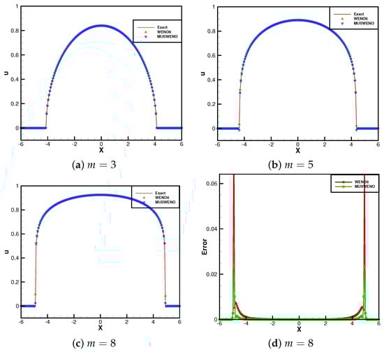
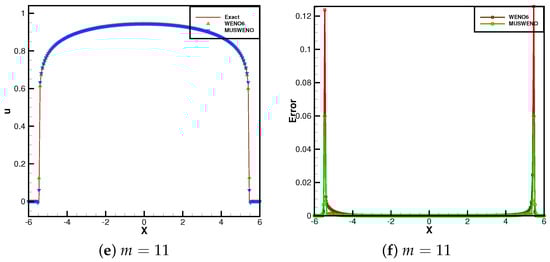
The porous medium equation is commonly employed to evaluate the numerical accuracy of schemes due to the availability of its exact solution. The initial condition is set as with boundary conditions . Figure 1 presents the numerical solutions computed with grid points for , and 11 at the final time , where the solid line represents the exact solution. The results demonstrate that both schemes yield comparable numerical solutions when m = 3 and 5. However, as m increases, the WENO6 scheme exhibits significantly larger errors, whereas the MUSWENO scheme maintains superior accuracy. Subfigures (d) and (f) in Figure 1 specifically compare the numerical errors of the two schemes at and , respectively, further illustrating the enhanced performance of the MUSWENO scheme for higher nonlinearity.
Figure 1.
Example 2. Barenblatt solution to the PME when m = 3, 5, 8, 11. t = 2.
Example 3.

We now examine the collision of two boxes with different heights. The physical context for this initial value problem involves interpreting the variable u as temperature, where the governing equation describes the behavior when two localized heat sources are abruptly introduced into distinct domains. Accordingly, we define the initial condition as
with the boundary condition for . The computational domain spans , discretized into 160 grid points. Figure 2 presents the numerical solution of the porous medium equation (PME) with at . Since this problem lacks an exact solution, we compare our results with the numerical solutions reported in [25], and observe that the profiles of the numerical solutions show good agreement. To demonstrate the superiority of the proposed MUSWENO scheme, we conduct comparative studies with both WENO6 and WENO8 schemes. The numerical results show significant improvement over WENO6 while being slightly inferior to WENO8.
Figure 2.
Example 3. Collision of two-box solution for PME.
Example 4.
Here, we investigate the convection–diffusion Buckley–Leverett equation [26], which plays a fundamental role in modeling two-phase flow in porous media:
where represents the saturation of the wetting phase, denotes the fractional flow function characterizing the convective transport, and the right-hand side models the capillary diffusion effects with being the nonlinear diffusion coefficient. In this example, the ε is set as 0.01 and we consider the following three cases for numerical testing:
Case 1:
The left boundary as and the right boundary can be extrapolated.
Case 2: The functions and remain the same as in Case 1, but with the following discontinuous initial condition:
Boundary conditions are and .
Case 3: The functions and remain the same as in Case 1, but due to gravitational effects, the convection term is modified to
Boundary conditions are and .
We conducted numerical simulations for these three cases, employing the WENO-JS scheme to discretize the convective term in the equation, while utilizing both the WENO6 and MUSWENO schemes for discretization of the diffusive term. Figure 3 shows all numerical results with 100 grid sizes at the final time . We use the numerical solution when the mesh number of the WENO6 scheme is encrypted to 800 as an exact solution for reference. Figure 3a,b present the simulation results for Case 1 using the two different schemes. The results clearly demonstrate that the MUSWENO scheme achieves better performance in regions with steep gradients. Similar conclusions were drawn for the other two cases.
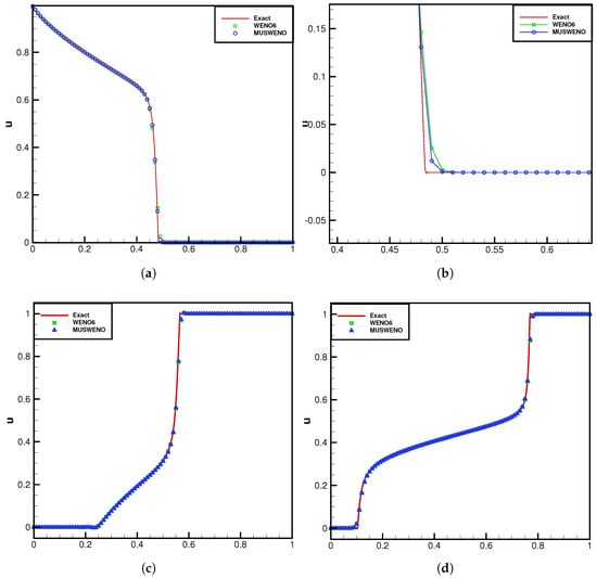
Figure 3.
Example 4. (a,b) shows the results of Case 1. (c,d) show the results of Case 2 and Case 3, respectively.
Example 5.
We investigate the numerical solution of a strongly degenerate parabolic convection–diffusion equation of the form
where controls the diffusion strength, and the convective flux is given by . The diffusion coefficient is defined piecewise:
This discontinuous coefficient leads to mixed hyperbolic-parabolic behavior: the equation becomes purely hyperbolic in regions where , while remaining parabolic elsewhere. The problem is solved with the initial condition
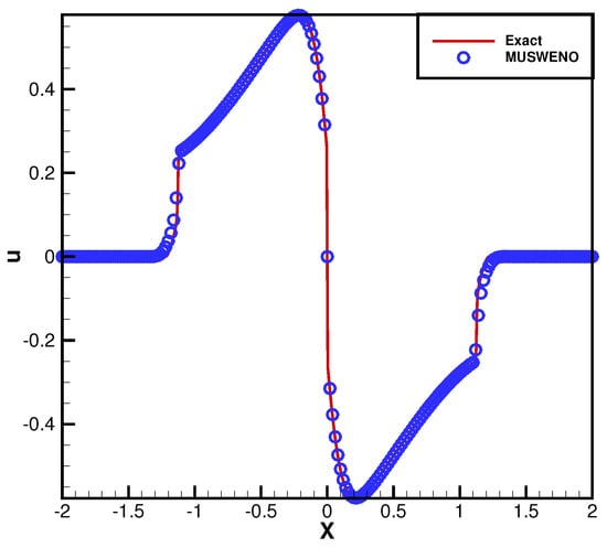
and homogeneous Dirichlet boundary conditions at both domain boundaries. We take the solution of the WENO6 schemes as the exact solution when the grid number is 800. The results of MUSWENO schemes with 200 grid sizes at time are shown in Figure 4. Numerical results show the high resolution and the accurate transition between the hyperbolic domain and the parabolic domain.
Figure 4.
Example 5. The Riemann problem for the strongly degenerate parabolic equation. T = 0.7.
Example 6.
Example 6. We consider a two-dimensional PME
with initial condition
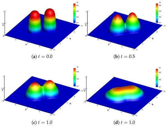
The periodic boundary conditions are applied in each directions. The numerical results of MUSWENO schemes at time t = 0.0, 0.5, 1.0, and 4.0 are shown in Figure 5. We can see that this scheme captures the sharp interface very well without introducing noticeable oscillations. The numerical results coincide well with that reported in [27].
Figure 5.
Example 6. 2D PME. From left to right, from top to bottom: the numerical results obtained using the MUSWENO scheme at , and 4. grid points.
Example 7.
We consider the two-dimensional Buckely–Leverett equation [28]
where represents the flux vector with components
and denotes the diffusion coefficient. The computational domain is discretized using a uniform grid of points, with periodic boundary conditions applied in both spatial directions. The initial condition is given by a circular discontinuity:
Figure 6 presents the numerical solutions obtained using the MUSWENO scheme, displaying both contour maps and surface plots. The results demonstrate excellent agreement with the reference solutions reported in [28], validating the accuracy and robustness of the numerical method.
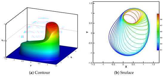
Figure 6.
Example 7. 2D Buckley–Leverett equation. The final time is . Contour and Surface the solution. Computational domain discretized with uniform grid points.
Example 8.
We study the two-dimensional strongly degenerate parabolic convection–diffusion equation
where , the convective flux , with , and the degenerate diffusion coefficient is defined in (49). The initial value is condition consists of two discontinuous circular patches:
Homogeneous Dirichlet boundary conditions are imposed on all domain boundaries. Using the same computational domain and mesh resolution as in Example 7, Figure 7 displays the numerical solutions at obtained by the MUSWENO scheme.
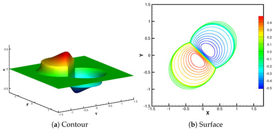
Figure 7.
Example 8. 2D strong parabolic equation. The final time is . Contour and Surface of the solution. Computational domain discretized with uniform grid points.
4. Concluding Remarks
In this paper, we propose a new mapped unequal-sized WENO (MUSWENO) scheme to solve nonlinear degenerate parabolic equations. We apply the idea to the approximation of the second-order derivative, and successfully achieve sixth-order accuracy in smooth domains. The newly developed nonlinear weights and mapping functions demonstrate significant improvements, delivering reduced numerical errors, enhanced resolution, and complete flexibility in linear weight selection. Future work will focus on implementing this framework within the Degasperis–Procesi equations.
Author Contributions
Z.H.: Writing—original draft. L.L.: Funding acquisition, Methodology, Supervision. All authors have read and agreed to the published version of the manuscript.
Funding
The research is partly supported by Henan Provincial Natural Science Foundation (No. 242300421392) and The Science and Technology Key Project of Henan Province of China (NO. 252102220057).
Data Availability Statement
Data available on request due to restrictions privacy reasons: The data presented in this study are available on request from the corresponding author. The raw numerical simulation data supporting this study’s findings are available upon request from the corresponding author due to their large size and specialized format requirements.
Conflicts of Interest
The authors declare no conflicts of interest.
References
- Aronson, D.G. The porous medium equation, in nonlinear diffusion problems. In Lecture Notes in Mathemathics 1224; Springer: Berlin/Heidelberg, Germany, 1986; pp. 1–46. [Google Scholar]
- Magenes, E.; Nochetto, R.H.; Verdi, C. Energy error estimates for a linear scheme to approximate nonlinear parabolic problems. RAIRO Math. Model. Numer. Anal. 1987, 21, 655–678. [Google Scholar] [CrossRef]
- Barenblatt, G.I. On self-similar motions of compressible fluid in a porous medium. Akad. Nauk SSR Prikl. Mat. Meh. 1952, 16, 679–698. [Google Scholar]
- Zeldovich, Y.B.; Kompaneetz, A.S. Towards a theory of heat conduction with thermal conductivity depending on the temperature. Collection of Papers Dedicated to the 70th Anniversary of AF Ioffe. Izd. Akad. Nauk SSSR Moscow 1950, 38, 61–72. [Google Scholar]
- Liu, X.-D.; Osher, S.; Chan, T. Weighted essentially non-pscillatory schemes. J. Comput. Phys. 1994, 115, 200–212. [Google Scholar] [CrossRef]
- Jiang, G.-S.; Shu, C.-W. Efficient implementation of weighted ENO schemes. J. Comput. Phys. 1996, 126, 202–228. [Google Scholar] [CrossRef]
- Zhu, J.; Qiu, J. A new fifth order finit difference WENO scheme for solving hyperbolic conservation laws. J. Comput. Phys. 2016, 318, 110–121. [Google Scholar] [CrossRef]
- Zhu, J.; Shu, C.-W. A new type of multi-resolution WENO schemes with increasingly higher order of accuracy. J. Comput. Phys. 2018, 375, 659–683. [Google Scholar] [CrossRef]
- Zhang, Y.T.; Shu, C.-W. Third order WENO scheme on three dimensional tetrahedral meshes. Commun. Comput. Phys. 2009, 5, 836–848. [Google Scholar]
- Zhang, Y.T.; Shu, C.-W. High order WENO schemes for Hamilton-Jacobi equations on triangular meshes. SIAM J. Sci. Comput. 2003, 24, 1005–1030. [Google Scholar] [CrossRef]
- Liu, Y.; Shu, C.-W.; Zhang, M. High order finite difference WENO schemes for nonlineat degenerate parabolic equations. SIAM J. Sci. Comput. 2011, 33, 939–965. [Google Scholar] [CrossRef]
- Shi, J.; Hu, C.; Shu, C.W. A technique of treating negative weights in WENO schemes. J. Comput. Phys. 2002, 175, 108–127. [Google Scholar] [CrossRef]
- Henrick, A.K.; Aslam, T.D.; Powers, J.M. Mapped weighted essentially non-oscillatory schemes: Achieving optimal order near critical points. J. Comput. Phys. 2005, 207, 542–567. [Google Scholar] [CrossRef]
- Abedian, R.; Adibi, H.; Dehghan, M. A high-order weighted essentially non-oscillatory (WENO) finite difference scheme for nonlinear degenerate parabolic equations. Comput. Phys. Commun. 2013, 184, 1874–1888. [Google Scholar] [CrossRef]
- Abedian, R. A new high-order weighted essentially non-oscillatory finite difference scheme for nonlinear degenerate parabolic equations. Numer. Methods Partial. Differ. Equ. 2021, 37, 1317–1343. [Google Scholar] [CrossRef]
- Abedian, R. WENO-Z Schemes with Legendre basis for non-linear degenerate parabolic equations. Iran J. Math. Sci. Inform. 2021, 16, 125–143. [Google Scholar] [CrossRef]
- Abedian, R.; Dehghan, M. A high-order weighted essentially nonoscillatory scheme based on exponential polynomials for nonlinear degenerate parabolic equations. Numer. Methods Partial. Differ. Equ. 2022, 38, 970–996. [Google Scholar] [CrossRef]
- Ahmat, M.; Qiu, J. Hybrid HWENO method for nonlinear degenerate parabolic equations. J. Sci. Comput. 2023, 96, 83. [Google Scholar] [CrossRef]
- Jiang, Y. High order finite difference multi-resolution WENO method for nonlinear degenerate parabolic equations. J. Sci. Comput. 2021, 86, 1–20. [Google Scholar] [CrossRef]
- Abedian, R.; Dehghan, M. A RBF-WENO finite difference scheme for non-linear degenerate parabolic equations. J. Sci. Comput. 2022, 93, 60. [Google Scholar] [CrossRef]
- Xu, Z.; Zhang, Y.T. High-order exponential time differencing multi-resolution alternative finite difference WENO methods for nonlinear degenerate parabolic equations. J. Comput. Phys. 2025, 529, 113838. [Google Scholar] [CrossRef]
- Castro, M.; Costa, B.; Don, W.S. High order weighted essentially non-oscillatory WENO-Z schemes for hyperbolic conservation laws. J. Comput. Phys. 2011, 230, 1766–1792. [Google Scholar] [CrossRef]
- Borges, R.; Carmona, M.; Costa, B.; Don, W.S. An improved weighted essentially non-oscillatory scheme for hyperbolic conservation laws. J. Comput. Phys. 2008, 227, 3191–3211. [Google Scholar] [CrossRef]
- Shu, C.-W. Total-variation-diminishing time discretizations. SIMA J. Sci. Stat. Comput. 1988, 9, 1073–1084. [Google Scholar] [CrossRef]
- Zhang, Q.; Wu, Z.L. Numerical simulation for porous medium equation by local discontinuous galerkun finite element method. J. Sci. Comput. 2009, 38, 127–148. [Google Scholar] [CrossRef]
- Buckley, S.E.; Leverett, M. Mechanism of fluid displacement in sands. Trans. AIME 1942, 146, 107–116. [Google Scholar] [CrossRef]
- Cavalli, F.; Naldi, G.; Puppo, G.; Semplice, M. High-order relaxation schemes for nonlinear degenerate diffusion problems. SIAM J. Numer. Anal. 2007, 45, 2098–2119. [Google Scholar] [CrossRef]
- Kurganov, A.; Tadmor, E. New high-resolution central schemes for nonlinear conservation laws and convection-diffusion equations. J. Comput. Phys. 2000, 160, 241–282. [Google Scholar] [CrossRef]


Disclaimer/Publisher’s Note: The statements, opinions and data contained in all publications are solely those of the individual author(s) and contributor(s) and not of MDPI and/or the editor(s). MDPI and/or the editor(s) disclaim responsibility for any injury to people or property resulting from any ideas, methods, instructions or products referred to in the content. |
© 2025 by the authors. Licensee MDPI, Basel, Switzerland. This article is an open access article distributed under the terms and conditions of the Creative Commons Attribution (CC BY) license (https://creativecommons.org/licenses/by/4.0/).