Abstract
Main roads are usually equipped with traffic flow monitoring devices in the road network to record the traffic flow data of the main roads in real time. Three complex scenarios, i.e., Y-junctions, multi-lane merging, and signalized intersections, are considered in this paper by developing a novel modeling system that leverages only historical main-road data to reconstruct branch-road volumes and identify pivotal time points where instantaneous observations enable robust inference of period-aggregate traffic volumes. Four mathematical models (I–IV) are built using the data given in appendix, with performance quantified via error metrics (RMSE, MAE, MAPE) and stability indices (perturbation sensitivity index, structure similarity score). Finally, the significant traffic flow change points are further identified by the PELT algorithm.
1. Introduction
In the road network, main roads are usually equipped with traffic flow monitoring devices, which can record the traffic flow data of the main roads in real time. When multiple branch roads converge into the main road, since some branch roads lack traffic flow monitoring devices, the traffic flow of each branch road needs to be estimated by combining the traffic flow data from the main road with the history trend information of the branch roads. This will provide data and methodological support for issues such as optimizing the timing of traffic signals, alleviating traffic congestion, and planning road resources.
A novel modeling framework that utilizes only historical main-road data is required to reconstruct branch-road traffic volumes and identify critical time points at which instantaneous observations facilitate robust inference of aggregate traffic volumes over specific time periods. And it must be applicable to several common real-world road scenarios, including Y-junctions, multi-lane merging, and signalized intersections, as well as to cases with noisy sensor data.
Least squares methods facilitate both linear and nonlinear economic forecasting, cross-category product gap analysis, and power system transmission line parameter estimation. The nonlinear variant has proven effective for estimating RC thermal models in building energy analysis. For complex optimization challenges, metaheuristic algorithms demonstrate wide applicability. Genetic algorithms optimize flexible power allocation in hybrid energy storage systems, enhance facial expression recognition via reinforcement learning, and improve tuned mass damper designs for wind turbine towers. Hybrid genetic-simulated annealing approaches minimize spare parts inspection costs, optimize composite laminate orientations, enable unsupervised tight sandstone reservoir classification, and refine least squares support vector machine parameters in breakdown diagnosis. Simulated annealing additionally supports tourism management optimization. Robust principal component analysis (RPCA) addresses critical image processing challenges, including single-image glow/hot-pixel removal and low-quality retinal image enhancement, while revealing methodological insights about outlier detection sensitivity to center-point inaccuracies. Change point detection algorithms analyze temporal dynamics across domains, examining both the impact of sliding window selection on detection accuracy and structural shifts in power grid time-series data. The PELT algorithm specifically enables precise microseismic signal identification. Most recently, hybrid models have performed outstandingly in regards to traffic prediction. Li et al. (2025) proposed a spatiotemporal graph model integrating CTM and transformer (the Cell Transformer, abbreviated as CeT) methods. CeT employs discretized lane segments to emulate the cell transmission model, creating a cell space to forecast vehicle counts across all segments based on historical traffic data [].
2. Materials and Methods
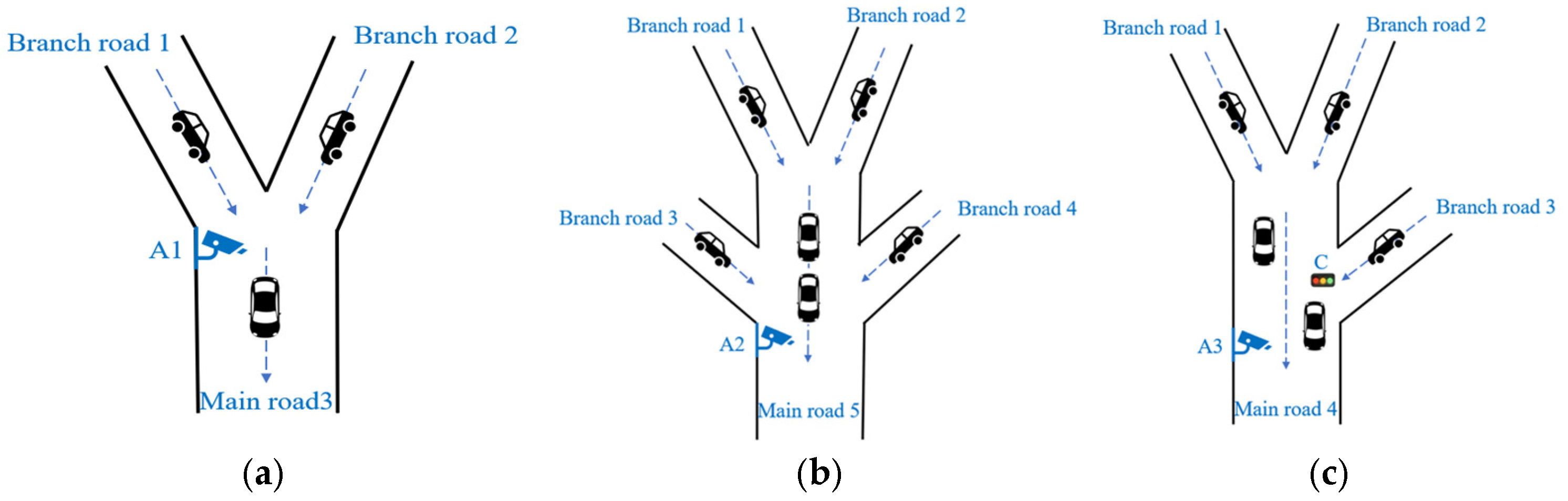
2.1. Scene Overviews
We consider the roads shown in the Figure 1. Firstly, the Y-shaped road in Figure 1a is investigated at the point where the traffic flow of Branch Road 1 and Branch Road 2 converges simultaneously into Main Road 3. Suppose that only the traffic flow monitoring device A1 is installed on Main Road 3, and the traffic flow information of the main road is recorded every 2 min. The time it takes for the vehicle to travel from the branch road to the main road and reach A1 is negligible. The third column in Table A1 in Appendix A provides the traffic flow data on Main Road 3 on a certain morning [6:58, 8:58] (7:00 is the first data recording moment, and 8:58 is the last data recording moment, as shown below).
Figure 1.
The three complex scenarios considered in this paper. (a) Y-shaped road; (b) The 4-branchs road; (c) The 3-branches road.
Secondly, consider the road shown in Figure 1b. The traffic flow of Branch Road 1 and Branch Road 2 converges onto Main Road 5 simultaneously, and the traffic flow of Branch Road 3 and Branch Road 4 converges onto Main Road 5 simultaneously. Only the traffic flow monitoring device A2 is installed on Main Road 5, and the traffic flow information of the main road is recorded once every 2 min. The fourth column in Table A1 in Appendix A provides the traffic flow data on Main Road 5 during the time period of [6:58, 8:58] on a certain morning. Suppose the time it takes for the vehicle to travel from the intersection of Branch Road 1 and Branch Road 2 to A2 is 2 min, and the travel time of the vehicle from Branch Road 3 and Branch Road 4 to A2 is negligible. According to the historical traffic flow observation records, during the time period of [6:58, 8:58], the traffic flow on Branch Road 1 was stable. The traffic volume of Branch Road 2 increased linearly during the time periods of [6:58, 7:48] and [8:14, 8:58], and remained stable during the time period of (7:48, 8:14). The traffic volume of Branch Road 3 first shows a trend of linear growth followed by stabilization. A periodic pattern is shown as the traffic volume on Branch Road 4. Thirdly, in Figure 1c, the traffic flow of Branch Road 1 and Branch Road 2 simultaneously converges onto Main Road 4. Branch Road 3 is a special traffic control road, and the vehicles on Branch Road 3 are controlled by the traffic signal C when passing through the intersection. The red light time for C is set to 8 min, the green light time to 10 min, and the yellow light time is negligible. Only the traffic flow monitoring device A3 is installed on Main Road 4, recording the traffic flow information of the main road every 2 min. The traffic flow data of Main Road 4 on a certain morning [6:58, 8:58] is provided in the fifth column in Table A1 of Appendix A. Suppose the driving time of the vehicle from the intersection of Branch Road 1 and Branch Road 2 to A3 is 2 min, and the driving time of the vehicle from Branch Road 3 to A3 is negligible.
Finally, in the case of a poor network signal, low visibility, large traffic flow, or too fast traffic speed, the traffic flow monitoring device may produce data errors. Considering the road shown in Figure 1c, suppose that the data recorded by device A3 on a certain day exhibits an error. The observed data within the time period of [6:58, 8:58] are shown in the sixth column in Table A1 of Appendix A. The traffic volume of Branch Road 1 exhibited a trend of “no flow → linear growth → stability → linear decrease to no flow”. The traffic volume of Branch Road 2 increased linearly and decreased linearly during the time periods of [6:58, 7:34] and [8:10, 8:58], respectively, and remained stable during the time period of (7:34, 8:10). The red light duration for signal light C is set to 8 min, the green light duration to 10 min, and the yellow light duration is negligible. When C shows a green light, the traffic flow on Branch Road 3 is either stable or shows a linear changing trend. When C shows a red light, the traffic volume on Branch Road 3 is 0. The time when C shows the green light is unknown.
2.2. Model Hypothesis
We propose the following hypothesis:
Assumption 1.
The traffic flow on the main road is the sum of the traffic flow on each branch road, and the traffic flow on each branch road displays a certain regularity (e.g., the morning and evening peaks; the traffic flow distribution is different during the weekday peak hours), and this regularity can be described by a function.
Assumption 2.
The roads are all one-way lanes, and the blue arrows in Figure 1 represent the direction of traffic flow.
Assumption 3.
The “increase/decrease” trend of traffic flow in scenarios 1–4 refers to the trend of “strictly monotonous increase/strictly monotonous decrease”, “stable” refers to a state in which the traffic flow remains constant at a non-negative fixed value, and the functional relationships describing the variations in traffic flow across all branches are continuous functions.
Assumption 4.
For convenience, let 7:00 be and in the functional relationship.
2.3. Model Analysis and Establishment
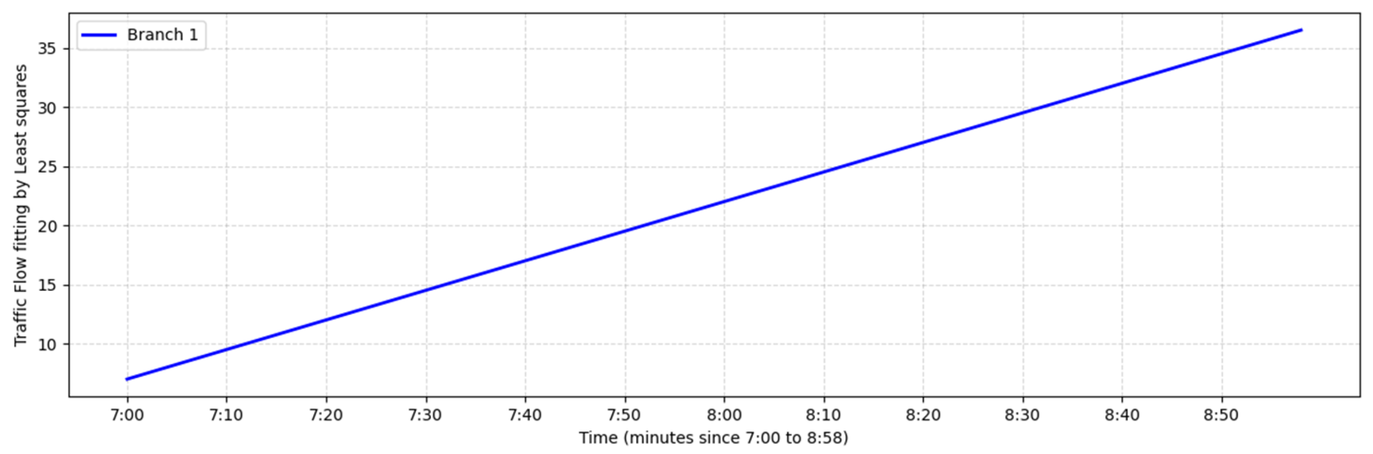
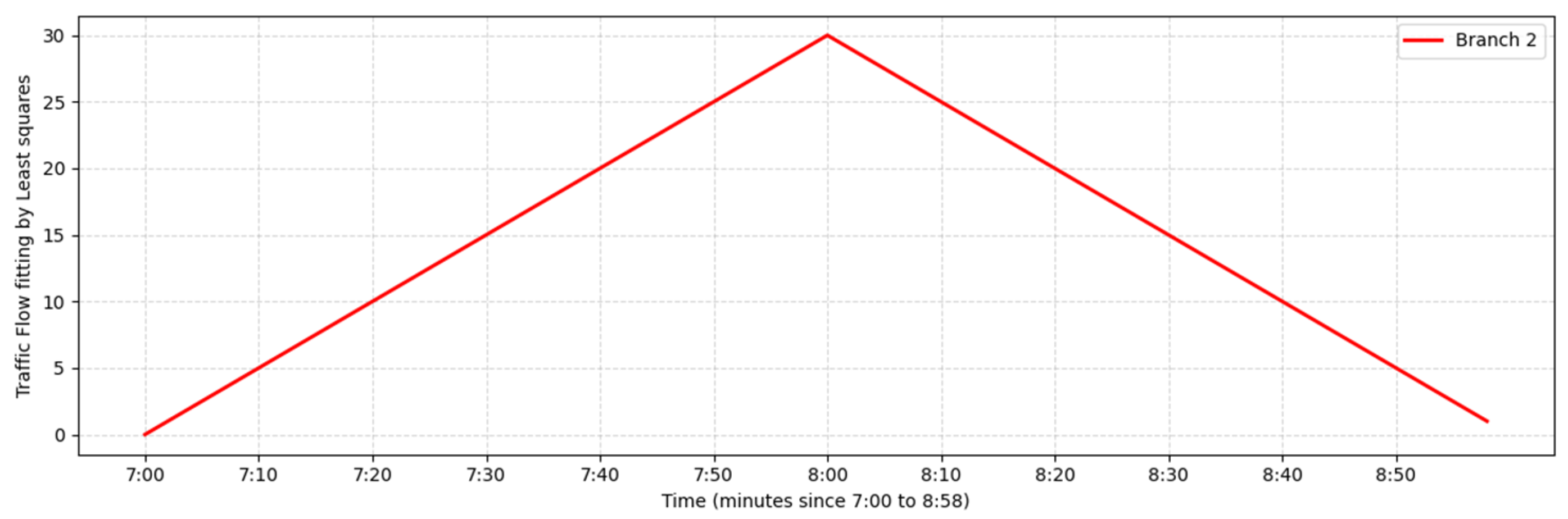
2.3.1. Mathematical Model I
According to the historical traffic flow observation records, during the period of [6:58, 8:58], the traffic flow on Branch Road 1 showed a linear growth trend, while that on Branch Road 2 exhibited a trend of linear growth first and then a linear decrease. For the empirical traffic flow data in the third column in Table A1 of Appendix A, we implemented a least squares curve fitting model [,,,] to reconstruct branch road traffic flows. Python 3.9 was utilized for algorithm implementation. Software implementation details include the least squares method coded in Python with NumPy (1.26.3) for matrix operations and SciPy (1.13.1) for optimization. Specifically, linear regression and piecewise linear models were developed for Branch Road 1 and Branch Road 2. The branch fitting formulas are shown in Equations (1) and (2). The resulting fitted curves are shown in Figure 2 and Figure 3, where RMSE is 0.0000, MAE is 0.000, and MAPE is 0%. Visualization of the main road traffic flow reveals an approximately linear trend. Consequently, the linear model for Branch Roads 1 and 2 achieves an RMSE of 0, indicating negligible overfitting. The fitted values of main road traffic flow align closely with observed data, demonstrating high model fidelity.
Figure 2.
The fitted results of branch 1 in Mathematical Model I.
Figure 3.
The fitted results of Branch Road 2 in Mathematical Model I.
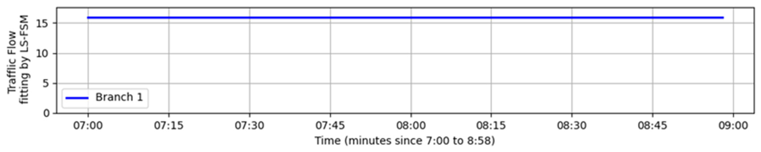
2.3.2. Mathematical Model II
According to the historical traffic flow observation records, during the time period of [6:58, 8:58], the traffic flow on Branch Road 1 was stable. The traffic volume of Branch Road 2 increases linearly during the time periods of [6:58, 7:48] and [8:14, 8:58], and remains stable during the time period of (7:48, 8:14). The traffic volume of Branch Road 3 shows a trend of linear growth first, followed by stabilization. The traffic volume on Branch Road 4 shows a periodic pattern.
For the dataset in the fourth column in Table A1 of Appendix A, we initialize model parameters using iterative algorithm outputs as estimates. These parameters were refined via nonlinear least squares optimization [], minimizing the residual sum of squares through iterative refinement. Following problem specifications, distinct functional forms were implemented for each branch: a constant model for Branch 1, piecewise linear models for Branches 2 and 3, and a Fourier series model (to capture periodic variations) for Branch 4. The Levenberg–Marquardt algorithm [] is used to fit the function model, where the regularization parameter is set 0.01, since the approximate effect is good. For Branch 4, we implemented a second-order Fourier spectral decomposition [,] containing fundamental and second harmonic terms, balancing accuracy with computational efficiency. Software implementation details are seen in Table A2. The branch fitting formulas are shown in Equations (3)–(6).
We obtain the fitted results and shown in Figure 3, Figure 4, Figure 5, Figure 6 and Figure 7, where RMSE is 3.6526, MAE is 3.0606, MAPE is 86.10%, PSI is 0.0861 under a 3% perturbation of the parameter, SSS is 99.68% with time delay compensation, and RMSE is 3.8152 without time delay compensation. Incorporating a 2 min time delay compensation significantly enhances model accuracy, as the resulting temporal patterns of branch road traffic flows demonstrably align with empirical traffic behavior. Residual analysis via the fast Fourier transform (FFT) method revealed no significant spectral peaks exceeding the statistical threshold (49.6105), confirming that the second-order expansion sufficiently captured inherent periodicity without higher-order terms.
Figure 4.
The fitted results of Branch Road 1 in Mathematical Model II.
Figure 5.
The fitted results of Branch Road 2 in Mathematical Model II.
Figure 6.
The fitted results of Branch Road 3 in Mathematical Model II.
Figure 7.
The fitted results of Branch Road 4 in Mathematical Model II.
Remark 1.
Perturbation Sensitivity Index:
We applied
±3% perturbations to the parameters of the branch road flow estimation function, recomputed the prediction error for main road traffic flow, and assessed the stability of the model’s output. Results indicate that the perturbation sensitivity index remains within the range of
±2 units across all tested perturbations, demonstrating robust model performance.
Structure Similarity Score:
The sign sequences (reflecting monotonicity properties) of branch functions are compared before and after perturbation, with structural similarity quantified. Experiments demonstrate that a structure similarity score exceeding 95% indicates that the model robustly preserves essential physical relationships in branch flow dynamics under data disturbances.
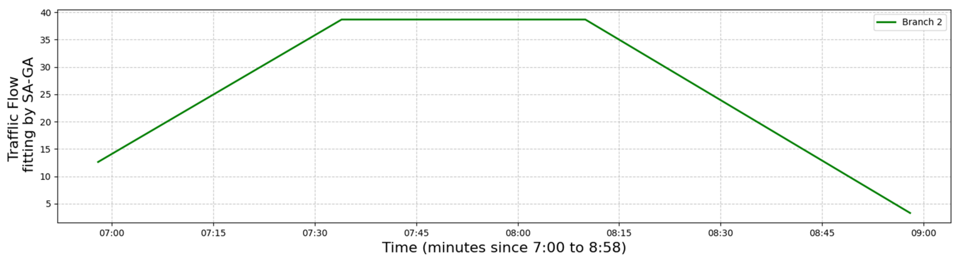
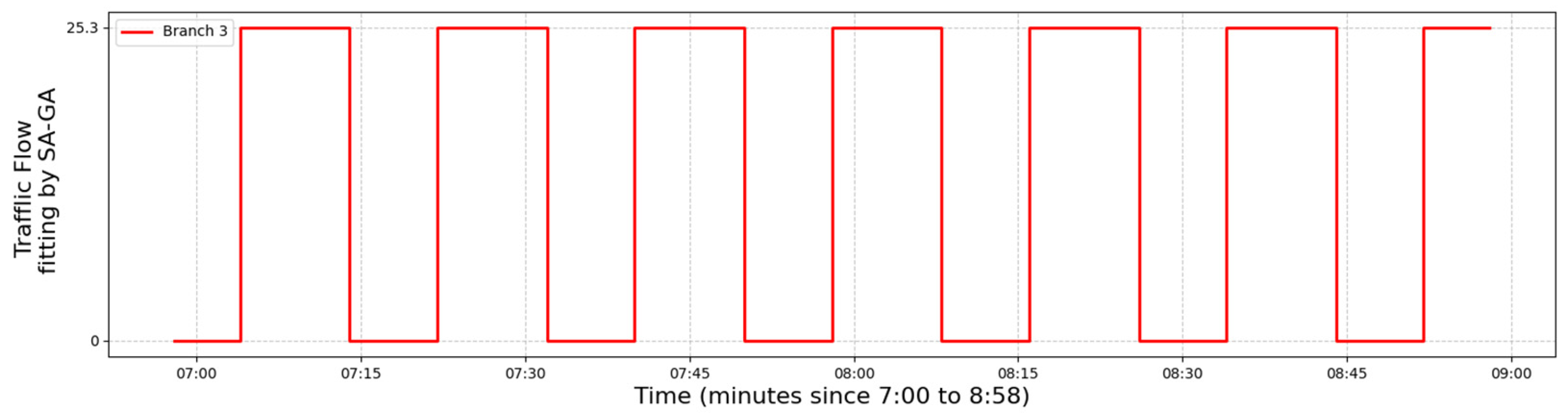
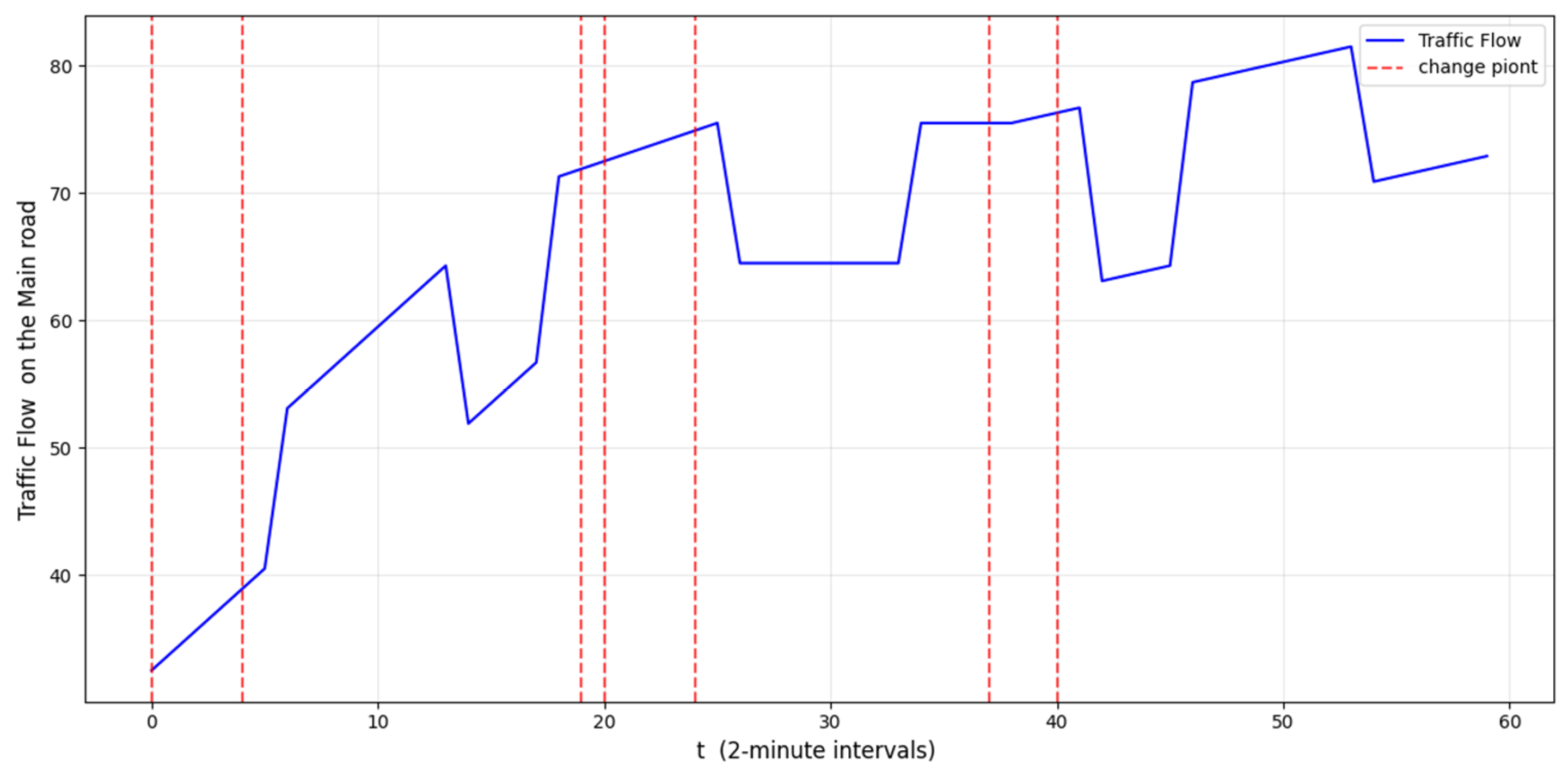
2.3.3. Mathematical Model III
According to the historical traffic flow observation records, during the time period of [6:58, 8:58], the traffic flow on Branch Road 1 exhibited a trend of “no flow→ increase → decrease → stability → decrease to no flow”. The traffic volume of Branch Road 2 increased linearly and decreased linearly during the time periods of [6:58, 8:10] and [8:34, 8:58], respectively, and remained stable during the time period of (8:10, 8:34). When C shows a green light, the traffic flow on Branch Road 3 either remains stable or shows a linear changing trend, and the first green light begins to light up at 7:06. When C shows a red light, the traffic volume on Branch Road 3 is 0. Based on the fact that hybrid models have recently performed outstandingly in regards to traffic prediction [,], this provides us with many ideas. However, these methods rely on multi-source sensors or other circumstances and cannot be fully applied to scenarios where there are no monitoring devices on branch roads.
For the dataset in the fifth column in Table A1 of Appendix A, we implemented constrained least squares estimation [] to determine parameter vectors by minimizing the residual sum of the squares. Piecewise linear models are subsequently established for Branches 1, 2, and 3, per problem requirements. When initial parameter adjustments failed to satisfy constraints for traffic flow on Branch 1, we integrated simulated annealing with nonlinear least squares (initial temperature: 1; step size: 0.5, adjusted every 50 iterations) to refine the model. Software implementation details are seen in Table A2. The branch fitting formulas are shown in Equations (9)–(11).
This hybrid approach fits the functional relationship well, with results presented in Figure 8, Figure 9 and Figure 10. RMSE is 11.9175, MAE is 9.4187, MAPE is 32.2188%, PSI is 0.4094, SSS is 99.76% under a 3% perturbation of the parameter with time delay compensation, and RMSE is 12.4331 without time delay compensation. The modeling error is primarily attributable to traffic flow discontinuities induced by signal control. Incorporating the 18 min signal cycle significantly enhances model accuracy, while the inferred branch road flow patterns align with empirical traffic characteristics.
Figure 8.
The fitted results of Branch Road 1 in Mathematical Model III.
Figure 9.
The fitted results of Branch Road 2 in Mathematical Model III.
Figure 10.
The fitted results of Branch Road 3 in Mathematical Model III.
2.3.4. Mathematical Model IV
According to the historical traffic flow observation records, in Figure 1c, the traffic volume of Branch Road 2 increased linearly and decreased linearly during the time periods of [6:58, 7:34] and [8:10, 8:58], respectively, and remained stable during the time period of (7:34, 8:10). The red light duration for signal light C is set to 8 min, the green light duration to 10 min, and the yellow light duration is negligible. When C shows a green light, the traffic flow on Branch Road 3 is either stable or shows a linear changing trend. When C shows a red light, the traffic volume on Branch Road 3 is 0. The time when C shows the green light is unknown.
We employ three parameter optimization methods: constrained least squares, a hybrid genetic algorithm–simulated annealing (GA–SA) approach [,,,,,,,], and robust principal component analysis (RPCA) [,,]. The hybrid GA–SA model was ultimately selected to characterize branch road traffic flows using the dataset in the sixth column in Table A1 of Appendix A. This hybrid algorithm enhances the classical simulated annealing framework by integrating the population-based search mechanism of genetic algorithms. The resulting optimizer combines probabilistic state transitions with global population search capabilities. In traffic monitoring applications, main road sensors may generate sparse yet high-amplitude errors due to network delays or equipment failures, resulting in sudden data drops. While the GA–SA hybrid fits functional traffic models, RPCA effectively isolates such anomalies while preserving the underlying low-rank traffic matrix structure.
In the GA–SA model, we set the population size to 15, the uniformly sampled mutation rate from 0.5 to 1.0, the crossover rate at 0.7, the initial temperature to 5230, and the restart temperature ratio to , after adjusting the parameters. In RPCA model, we set the regularization coefficient to . Software implementation details can be seen in Table A2 The branch fitting formulas are shown in Equations (12)–(14). The GA–SA model displays the best effect, and the result is shown in Figure 11, Figure 12 and Figure 13. Meanwhile the green light first commenced at 7:06 (t = 3). In the GA–SA model, RMSE is 13.6733, MAE is 2.8329, MAPE is 7.42%, PSI is 0.0184, SSS is 99.89% under a 3% perturbation of the parameter with time delay compensation, and RMSE is 4.6824 without time delay compensation. The error indexes and model stability indexes for NLS and RPCA are shown in Table A2 of Appendix B.
Figure 11.
The fitted results of Branch Road 1 in Mathematical Model IV.
Figure 12.
The fitted results of Branch Road 2 in Mathematical Model IV.
Figure 13.
The fitted results of Branch Road 3 in Mathematical Model IV.
3. Results
According to the expression of Mathematical Model I to Mathematical Model IV, we obtain the traffic flow values on each branch road at moment 7:30 and 8:30, respectively (see Table 1, Table 2, Table 3 and Table 4).
Table 1.
Numerical values of branch traffic flow in Mathematical Model I.
Table 2.
Numerical values of branch traffic flow in Mathematical Model II.
Table 3.
Numerical values of branch traffic flow in Mathematical Model III.
Table 4.
Numerical values of branch traffic flow in Mathematical Model IV.
Furthermore, to determine function parameters, sufficient data points surrounding these key time points are required. Therefore, change point detection [,] is employed to identify optimal segmentation intervals. Specifically, the PELT algorithm [] is applied to the main road traffic flow time series to detect significant change points.
Let the main road traffic sequence be and find the set of change points , such that the residuals of the segmented linear model are minimized, as follows:
where is the segmented cost function (e.g., mean square error), and is the penalty coefficient, which controls the number of change points. Figure 14 presents the results for Model II, identifying change points at times t = 0, 4, 19, 25, 37, 40 and observation times 07:00, 07:08, 07:38, 07:50, 08:14, 08:20. The penalty coefficient is set to 3, resulting in the lowest MAE of 3.38. For Mathematical Model III, which is presented in Figure 15, the detected change points occur at t = 3, 8, 12, 17, 21, 26, 30, 35, 39, 44, 48, 53, 57, with observations recorded at 07:06, 07:16, 07:24, 07:34, 07:42, 07:52, 08:00, 08:10, 08:18, 08:28, 08:36, 08:46, 08:54. The penalty coefficient is set to 8, resulting in the lowest MAE of 8.29. Model IV, which is presented in Figure 16, yields change points at t = 3, 8, 12, 17, 19, 21, 26, 30, 35, 39, 44, 48, 49, 53, 57 and observations at 07:06, 07:16, 07:24, 07:34, 07:38, 07:42, 07:52, 08:00, 08:10, 08:18, 08:28, 08:36, 08:38, 08:46, 08:54. The penalty coefficient is set to 3, resulting in the lowest MAE of 10.27. Software implementation details include the PELT algorithm coded in Python with NumPy, ruptures (1.1.9) for signal segmentation and pandas (2.3.0) for data processing.
Figure 14.
The moments of variation points and the observation moments in Mathematical Model II.
Figure 15.
The moments of variation points and the observation moments in Mathematical Model III.
Figure 16.
The moments of variation points and the observation moments in Mathematical Model IV.
4. Discussion
Collectively, Models I-IV underpin the development of comprehensive traffic monitoring systems. Crucially, the robust optimization framework derived from Model IV enables practical implementation within smart city infrastructures by
- (1)
- Rapid identification of incident locations;
- (2)
- Dynamic generation of optimal rerouting strategies.
5. Conclusions
This paper has four main limitations:
- (1)
- The strict monotonicity of traffic flow assumed in Assumption 3 may not hold in actual road conditions;
- (2)
- The fixed signal timing in Model III/IV reduces adaptability to adaptive signal systems;
- (3)
- The computational complexity of the GA–SA hybrid limits real-time deployment (>2 s/iteration);
- (4)
- The validation datasets lack extreme weather conditions. Future work will integrate reinforcement learning for dynamic signal optimization.
Nevertheless, The model proposed in this study exhibits high adaptability, featuring multi-class configurations tailored for diverse road structures and complex constraints. Algorithmically, this work introduces three key innovations:
- (1)
- Periodic fluctuation modeling through the Fourier spectral method.
- (2)
- Constrained optimization for enforcing continuity in piecewise functions.
- (3)
- Hybrid global optimization combining genetic algorithms with simulated annealing.
These advancements collectively enhance the model’s explanatory capability and generalization performance. Furthermore, the variable change-point detection algorithm quantitatively identifies critical monitoring moments, providing a cost-efficient framework for practical traffic data collection.
Author Contributions
B.W.: formal analysis, methodology, writing—original draft, and writing—review and editing; S.Z.: formal analysis and software. All authors have read and agreed to the published version of the manuscript.
Funding
This research received no external funding.
Data Availability Statement
The data used in this study are available.
Acknowledgments
The authors would like to thank the manuscript readers for their very professional comments and helpful suggestions.
Conflicts of Interest
The authors declare no conflicts of interest.
Appendix A
Table A1.
Traffic flow on the main roads considered in this paper (obtained from the 2025 May Day MCM (Mathematical Contest in Modeling) in China).
Table A1.
Traffic flow on the main roads considered in this paper (obtained from the 2025 May Day MCM (Mathematical Contest in Modeling) in China).
| Moment | Time | Traffic Flow on Main Road 3 in Figure 1a | Traffic Flow on Main Road 5 in Figure 1b | Traffic Flow on Main Road 4 in Figure 1c | Traffic Flow on Main Road 4 in Figure 1c |
|---|---|---|---|---|---|
| 07:00 | 0 | 7.00 | 32.5 | 0.8 | 20.1178 |
| 07:02 | 1 | 8.50 | 34.1 | 2 | 21.6463 |
| 07:04 | 2 | 10.00 | 35.7 | 3.2 | 31.0159 |
| 07:06 | 3 | 11.50 | 37.3 | 4.4 | 40.5070 |
| 07:08 | 4 | 13.00 | 38.9 | 34.6 | 41.4589 |
| 07:10 | 5 | 14.50 | 40.5 | 37.3 | 40.3803 |
| 07:12 | 6 | 16.00 | 53.1 | 40 | 45.0280 |
| 07:14 | 7 | 17.50 | 54.7 | 42.7 | 23.5751 |
| 07:16 | 8 | 19.00 | 56.3 | 45.4 | 27.6601 |
| 07:18 | 9 | 20.50 | 57.9 | 20.625 | 28.5191 |
| 07:20 | 10 | 22.00 | 59.5 | 30.31 | 22.8609 |
| 07:22 | 11 | 23.50 | 61.1 | 39.395 | 54.4147 |
| 07:24 | 12 | 25.00 | 62.7 | 47.82 | 56.3573 |
| 07:26 | 13 | 26.50 | 64.3 | 81.075 | 54.6330 |
| 07:28 | 14 | 28.00 | 51.9 | 87.35 | 59.2022 |
| 07:30 | 15 | 29.50 | 53.5 | 92.785 | 55.9851 |
| 07:32 | 16 | 31.00 | 55.1 | 97.32 | 37.2741 |
| 07:34 | 17 | 32.50 | 56.7 | 100.895 | 43.2759 |
| 07:36 | 18 | 34.00 | 71.3 | 81.15 | 44.3377 |
| 07:38 | 19 | 35.50 | 71.9 | 83.275 | 46.9259 |
| 07:40 | 20 | 37.00 | 72.5 | 84.26 | 74.7459 |
| 07:42 | 21 | 38.50 | 73.1 | 84.045 | 69.1357 |
| 07:44 | 22 | 40.00 | 73.7 | 109.97 | 74.9930 |
| 07:46 | 23 | 41.50 | 74.3 | 106.375 | 75.0219 |
| 07:48 | 24 | 43.00 | 74.9 | 101.4 | 72.3299 |
| 07:50 | 25 | 44.50 | 75.5 | 101.8 | 52.8119 |
| 07:52 | 26 | 46.00 | 64.5 | 102.2 | 53.9451 |
| 07:54 | 27 | 47.50 | 64.5 | 79.2 | 52.3878 |
| 07:56 | 28 | 49.00 | 64.5 | 80.4 | 55.7438 |
| 07:58 | 29 | 50.50 | 64.5 | 81.6 | 81.1195 |
| 08:00 | 30 | 52.00 | 64.5 | 82.8 | 86.6484 |
| 08:02 | 31 | 51.50 | 64.5 | 108.8 | 81.2547 |
| 08:04 | 32 | 51.00 | 64.5 | 110.8 | 83.2154 |
| 08:06 | 33 | 50.50 | 64.5 | 112.8 | 81.3694 |
| 08:08 | 34 | 50.00 | 75.5 | 110.2 | 53.7771 |
| 08:10 | 35 | 49.50 | 75.5 | 107.6 | 59.5877 |
| 08:12 | 36 | 49.00 | 75.5 | 76.2 | 58.5586 |
| 08:14 | 37 | 48.50 | 75.5 | 71.6 | 54.5368 |
| 08:16 | 38 | 48.00 | 75.5 | 67 | 80.8018 |
| 08:18 | 39 | 47.50 | 75.9 | 62.4 | 71.8756 |
| 08:20 | 40 | 47.00 | 76.3 | 76.8 | 73.5100 |
| 08:22 | 41 | 46.50 | 76.7 | 72.2 | 68.9525 |
| 08:24 | 42 | 46.00 | 63.1 | 67.6 | 67.9241 |
| 08:26 | 43 | 45.50 | 63.5 | 63 | 44.8616 |
| 08:28 | 44 | 45.00 | 63.9 | 63 | 36.4950 |
| 08:30 | 45 | 44.50 | 64.3 | 44 | 35.4181 |
| 08:32 | 46 | 44.00 | 78.7 | 44 | 31.5647 |
| 08:34 | 47 | 43.50 | 79.1 | 44 | 71.6705 |
| 08:36 | 48 | 43.00 | 79.5 | 44 | 68.6749 |
| 08:38 | 49 | 42.50 | 79.9 | 82.15 | 65.5375 |
| 08:40 | 50 | 42.00 | 80.3 | 82.3 | 58.2082 |
| 08:42 | 51 | 41.50 | 80.7 | 82.45 | 60.4376 |
| 08:44 | 52 | 41.00 | 81.1 | 82.6 | 17.2408 |
| 08:46 | 53 | 40.50 | 81.5 | 82.75 | 12.3009 |
| 08:48 | 54 | 40.00 | 70.9 | 38.9 | 10.9520 |
| 08:50 | 55 | 39.50 | 71.3 | 38.05 | 12.9869 |
| 08:52 | 56 | 39.00 | 71.7 | 37.2 | 36.8780 |
| 08:54 | 57 | 38.50 | 72.1 | 36.35 | 31.1231 |
| 08:56 | 58 | 38.00 | 72.5 | 52.5 | 32.2821 |
| 08:58 | 59 | 37.50 | 72.9 | 51.65 | 28.5905 |
Appendix B
Table A2.
The error indexes and model stability indexes for each method.
Table A2.
The error indexes and model stability indexes for each method.
| Model | II | III | IV | ||
|---|---|---|---|---|---|
| Method | LS-FSM | SA-NLS | NLS | GA–SA | RPCA |
| Software implementation details | NumPy pandas SciPy scikit-learn (1.6.1) | NumPy pandas SciPy | NumPy pandas SciPy scikit-learn | NumPy pandas SciPy scikit-learn | NumPy pandas scikit-learn CVXPY (1.6.6) |
| RMSE | 3.6526 | 11.9175 | 10.7004 | 3.6733 | 5.8200 |
| MAE | 3.0606 | 9.4187 | 8.0558 | 2.8329 | 3.6315 |
| MAPE | 5.0600% | 32.2188% | 20.6800% | 7.4200% | 10.5100% |
| PSI | 0.0861 | 0.4094 | 0.1284 | 0.0184 | 0.0200 |
| SSS | 99.68% | 99.76% | 99.44% | 99.89% | 97.96% |
| RMSE without time delay compensation | 3.8152 | 12.4331 | 10.9357 | 4.6824 | 7.6431 |
References
- Li, A.R.; Xu, Z.L.; Li, W.H.; Chen, Y.Y.; Pan, Y.Y. Urban Signalized Intersection Traffic State Prediction: A Spatial-Temporal Graph Model Integrating the Cell Transmission Model and Transformer. Appl. Sci. 2025, 15, 2377. [Google Scholar] [CrossRef]
- Shintani, M. Nonlinear forecasting analysis using diffusion indexes: An application to Japan. J. Money Credit. Bank. 2005, 37, 517–538. [Google Scholar] [CrossRef]
- Smalter Hall, A.; Cook, T.R. Macroeconomic Indicator Forecasting with Deep Neural Networks; Technical Report 17–11; Federal Reserve Bank of Kansas City: Kansas City, MO, USA, 2017. [Google Scholar]
- Yan, B.; Cao, L.J.; Zhao, C.X. Analysis Method of Transmission Line Parameter Estimation Based on Linear Least Squares Regression and PMU Data. Chin. J. Electron Devices 2024, 47, 1362–1367. (In Chinese) [Google Scholar]
- Zamani, V.; Abtahi, S.; Chen, Y.X.; Li, Y. Parameter-input estimation of RC thermal models of buildings using unscented Kalman filter and nonlinear least square method. Indoor Built Environ. 2025, 34, 41–75. [Google Scholar] [CrossRef] [PubMed]
- Kumar, M.D.; Jawad, M.; Ramanuja, M.; Ghodhbani, R.; Yook, S.J.; Abdallah, S.A.O. Forecasting heat and mass transfer enhancement in magnetized non-Newtonian nanofluids using Levenberg-Marquardt algorithm: Influence of activation energy and bioconvection. Mech. Time Depend. Mater. 2024, 29, 14. [Google Scholar] [CrossRef]
- Lovett, N.; Bhatt, H.P. Efficiently and accurately simulating multi-dimensional M-coupled nonlinear Schrödinger equations with fourth-order time integrators and Fourier pseudo-spectral method. Int. J. Comput. Math. 2025, 102, 653–677. [Google Scholar] [CrossRef]
- Zhang, J.; Dong, L.X.; Zhang, Z.R. Second-order scalar auxiliary variable Fourier-spectral method for a liquid thin film coarsening model. Math. Methods Appl. Sci. 2023, 46, 18815–18836. [Google Scholar] [CrossRef]
- Venkataraman, S.; Rumpler, R. Urban traffic flow estimation with noise measurements using log-linear regression. Appl. Acoust. 2025, 236, 110745. [Google Scholar] [CrossRef]
- Graffelman, J.; Bruce, S.W.; Goudet, J. Estimation of Jacquard’s genetic identity coefficients with bi-allelic variants by constrained least-squares. Heredity 2024, 134, 10–20. [Google Scholar] [CrossRef]
- Ma, B.; Li, H.P. Optimal flexible power allocation energy management strategy for hybrid energy storage system with genetic algorithm based model predictive control. Energy 2025, 324, 135958. [Google Scholar] [CrossRef]
- Altaha, M.A.; Jarraya, I.; Haddad, L.; Hamdani, T.M.; Chabchoub, H.; Alim, A.M. RLGA-FER: Reinforcement learning based on genetic algorithm for facial expression recognition enhancing. Int. J. Mach. Learn. Cybern. 2024. preprint. [Google Scholar] [CrossRef]
- Wang, Y.X.; Huang, Y.; Chen, F. Optimisation of Spare Parts Quality Inspection Cost Based on Simulated Annealing and Genetic Algorithm. Front. Comput. Intell. Syst. 2024, 10, 48–53. [Google Scholar] [CrossRef]
- Arellano, M.T.; Vergara, A.B.; Gonzalez, S.P.; Hernández, E.C.H.; Edgar, A.; Franco Ur quiza, E.A. Optimal design of laminates orientation in a composite material by genetics algorithm and simulated annealing. Mech. Adv. Mater. Struct. 2024, 31, 10592–10600. [Google Scholar] [CrossRef]
- Wu, B.H.; Xie, R.H.; Xiao, L.Z.; Guo, J.F.; Jin, G.W.; Fu, J.W. Integrated classification method of tight sandstone reservoir based on principal component analysis simulated annealing genetic algorithm—fuzzy cluster means. Pet. Sci. 2023, 20, 2747–2758. [Google Scholar] [CrossRef]
- Zhang, D.W.; Li, W.L.; Wang, C.G.; Li, J.H. Simulation research on breakdown diagnosis based on least squares support vector machine optimized by simulated annealing genetic algorithm. Int. J. Model. Simul. Sci. Comput. 2024, 15, 2350046. [Google Scholar] [CrossRef]
- Li, S.Z.; Zhou, X.H.; Zhang, X.S.; Wang, Y.H.; Jiang, L.M. Optimization of Tuned Mass Damper for Steel–Concrete Hybrid Wind Turbine Tower Using Genetic Algorithm. Int. J. Struct. Stab. Dyn. 2024. preprint. [Google Scholar] [CrossRef]
- Li, H.Z.; Zhang, Z.Y.; Huang, Y.H.; Lin, Z.H.; Lei, Z. Analysis of Tourism Management Based on Genetic Algorithm and Simulated Annealing Algorithm. World Sci. Res. J. 2025, 11, 133–141. [Google Scholar]
- Zhang, Y.H.; Zhang, H.F.; Liu, Z.Y.; Zhu, J.; Gu, J.Y.; Wang, X.B.; Zhu, Z.Y.; Tang, Y.J.; Wang, J. Glow and hot pixels removal using improved robust principal component analysis. J. Electron. Imaging 2023, 32, 043012. [Google Scholar] [CrossRef]
- Wan, G.H.; He, B.; Schweitzer, H. The art of centering without centering for robust principal component analysis. Data Min. Knowl. Discov. 2023, 38, 699–724. [Google Scholar] [CrossRef]
- Likassa, H.T.; Chen, D.-G.; Chen, K.; Wang, Y.; Zhu, W. Robust PCA with Lw,∗ and L2,1 Norms: A Novel Method for Low-Quality Retinal Image Enhancement. J. Imaging 2024, 10, 151. [Google Scholar] [CrossRef]
- Kou, A.Q.; Cheng, Y.; Huang, X.Y.; Jin, J. Dynamic replenishment policy for perishable goods using change point detection-based soft actor-critic reinforcement learning. Expert Syst. Appl. 2025, 270, 126556. [Google Scholar] [CrossRef]
- Bouman, R.; Schmeitz, L.; Buise, L.; Heres, J.; Shapovalova, Y.; Heskes, T. Acquiring better load estimates by combining anomaly and change point detection in power grid time-series measurements. Sustain. Energy Grids Netw. 2024, 40, 101540. [Google Scholar] [CrossRef]
- Wang, X.L.; Lv, M.H. Research on the Initial Arrival Recognition and Judgment Method of Microseismic Signals Based on PELT. Pure Appl. Geophys. 2024, 182, 1263–1278. [Google Scholar] [CrossRef]
Disclaimer/Publisher’s Note: The statements, opinions and data contained in all publications are solely those of the individual author(s) and contributor(s) and not of MDPI and/or the editor(s). MDPI and/or the editor(s) disclaim responsibility for any injury to people or property resulting from any ideas, methods, instructions or products referred to in the content. |
© 2025 by the authors. Licensee MDPI, Basel, Switzerland. This article is an open access article distributed under the terms and conditions of the Creative Commons Attribution (CC BY) license (https://creativecommons.org/licenses/by/4.0/).