Abstract
Speaker profiling systems are often evaluated on a single corpus, which complicates reliable comparison. We present a fully reproducible evaluation pipeline that trains Convolutional Neural Networks (CNNs) and Long-Short Term Memory (LSTM) models independently on three speech corpora representing distinct recording conditions—studio-quality TIMIT, crowdsourced Mozilla Common Voice, and in-the-wild VoxCeleb1. All models share the same architecture, optimizer, and data preprocessing; no corpus-specific hyperparameter tuning is applied. We perform a detailed preprocessing and feature extraction procedure, evaluating multiple configurations and validating their applicability and effectiveness in improving the obtained results. A feature analysis shows that Mel spectrograms benefit CNNs, whereas Mel Frequency Cepstral Coefficients (MFCCs) suit LSTMs, and that the optimal Mel-bin count grows with corpus Signal Noise Rate (SNR). With this fixed recipe, EfficientNet achieves 99.82% gender accuracy on Common Voice (+1.25 pp over the previous best) and 98.86% on VoxCeleb1 (+0.57 pp). MobileNet attains 99.86% age-group accuracy on Common Voice (+2.86 pp) and a 5.35-year MAE for age estimation on TIMIT using a lightweight configuration. The consistent, near-state-of-the-art results across three acoustically diverse datasets substantiate the robustness and versatility of the proposed pipeline. Code and pre-trained weights are released to facilitate downstream research.
1. Introduction
In the current era, automatically characterizing a person from their voice signal has gained increasing importance. This process is fundamental in a world dominated by human-machine interactions, where individuals use digital means to express emotions, desires, and preferences. This research area has acquired great relevance, especially in applications such as voice communication systems, where understanding the interlocutor’s profile can enhance the quality of the service offered.
Voice-machine interaction systems, like Interactive Voice Response (IVR), have been used to provide information and services based on the speaker’s responses. However, with current scientific and technological advancements, more advanced systems have emerged, such as Automatic Speaker Profiling (ASP), which utilizes artificial intelligence (AI) to extract speaker characteristics such as age, gender, emotions, race, and others, thereby personalizing the user experience more effectively [1,2].
Implementing a gender and age classification system using neural networks is important for several reasons. One of them is that it has applications in industry and commerce, as many companies can benefit from the ability to automatically classify their customers by gender and age. This allows for better market segmentation, product and service personalization, and more effective marketing strategies. In security and surveillance environments, such as airports or public transportation stations, the ability to identify people’s gender and age can be useful for enhancing security and applying appropriate control measures because a gender and age classification system can improve the accuracy in identifying individuals, which could reduce security incidents. In the health field, an accurate gender and age classification system can assist in medical and epidemiological research, allowing for a better understanding of how certain diseases or health conditions affect different demographic groups. Beyond their utility in commercial applications, these characteristics are also fundamental in fields like forensic research, where they can help to identify distinctive traits of an individual through their voice [3,4,5].
The development of classification and regression systems to determine a person’s gender and age from their voice signal has been a subject of research for years. Various techniques and models exist to address this task, aiming to increase accuracy and reduce errors to achieve optimal results [5,6]. However, despite advancements in this field, significant challenges persist, such as variability in voice characteristics due to factors like accent, audio quality, and recording context. Therefore, it is necessary to continue researching and developing more robust and accurate approaches for the automatic characterization of individuals from their voice signal [7].
The main objective of our approach is obtaining a base trained model in three different datasets for the classification and estimation of gender and age from speech signals. Each corpus has their own characteristics that support robustness and generalization for speaker profiling tasks. The dataset’s language is English, and they have a variety of accents and dialects, with native and non-native English speakers. To achieve our goal, we study various configurations of Deep Neural Networks (DNNs), specifically Long Short-Term Memory (LSTM) and Convolutional Neural Networks (CNNs) for gender and age classification and estimation. We employ pre-trained CNN models and different configurations of LSTM to analyze their performance across datasets. Although, we propose a comprehensive preprocessing and feature extraction methodology aimed at addressing existing limitations in current approaches. By systematically evaluating multiple feature configurations, we validate the effectiveness and applicability of our proposed method. Our approach not only facilitates improved data representation but also demonstrably enhances overall performance metrics, as evidenced by experimental validation. The main objective is to train and evaluate different approaches to achieve competitive results in classification and estimation accuracies compared to the state of the art. These trained models could be the basis of an end-to-end framework that could achieve a better tradeoff between accuracy and generalization ability across different speech tasks. To this end, the system will be tested on three different speech datasets, aiming to assess its robustness and capacity to generalize across diverse acoustic and demographic conditions.
The rest of this paper is organized as follows: Section 2 describes related work, and Section 3 describes the proposed method. Section 4 explores the datasets’ composition in detail and shows the experimental results, and finally, we elaborate on the conclusions of this work and future works that may arise from this work in Section 5.
2. Related Work
Speaker profiling, specifically age and gender classification, has attracted considerable research interest due to its broad applicability in human-computer interaction, forensic analysis, and personalized services. Prior studies have extensively investigated methods that utilize voice signals, recognized as a valuable source of speaker-specific characteristics. This section reviews current techniques categorized into traditional machine learning approaches and recent advancements leveraging deep learning models, particularly DNNs.
In the domain of age classification, several methodologies have been proposed. Reference [8] introduced two distinct approaches: one employing Mel spectrogram images processed via a CNN, and another that extracted acoustic features, including Mel Frequency Cepstral Coefficients (MFCCs), Spectral Contrast, and Spectral Roll-Off, classified using K-Nearest Neighbors (KNN) [9] and Label Propagation (LP) [10]. Similarly, the work described in [11] explored various architectures, notably Temporal Convolutional Neural Networks (TCNs), Convolutional Recurrent Neural Networks (CRNNs), and CNNs, alongside traditional techniques such as Support Vector Regression (SVR) and Random Forest classifiers.
Advancements in speaker embedding have also demonstrated considerable improvements in accuracy. For instance, [12] utilized embedder architectures such as x-vector and d-vector systems combined with multi-stage transfer learning, achieving state-of-the-art age estimation results on the TIMIT dataset. The challenge of accurately estimating speaker age from “in-the-wild” speech data was explicitly addressed in [13], which enriched the VoxCeleb datasets with speaker age labels and examined multiple feature representations (i-vectors, x-vectors, log-mel filters, and MFCCs) coupled with classifiers like logistic regression, ridge regression, and CNN-based models.
Gender classification has similarly benefited from deep learning innovations. The analysis in [11] highlighted the superiority of deep learning methods compared to traditional machine learning models trained on handcrafted features. Further enhancing classification capabilities, the work by [14] proposed an end-to-end CNN architecture incorporating a Multiple Attention Module (MAM) to extract both spatial and temporal features, demonstrating joint and individual classifications for gender and age on the Mozilla Common Voice dataset.
Multitask learning and data augmentation techniques have been integral in recent approaches to improving classification accuracy. Reference [15] proposed multitask learning utilizing CNN-ResNet with attentive statistical pooling and fine-tuning strategies, employing Label Distribution Smoothing and focal loss techniques to manage class imbalance effectively. Additionally, Ref. [16] combined CNN models with spectral data augmentation, specifically applying random frequency masking, to enhance feature robustness. Furthermore, Ref. [17] demonstrated improved age classification by initially performing gender classification with a Multi-layer Perceptron (MLP), subsequently training ResNet34 and x-vector models separately for each gender.
Hybrid methods integrating classical machine learning with deep learning architectures have also shown promising results. Reference [18] implemented gender classification using a DNN while employing classical approaches like Robust-Scaler, Principal Component Analysis (PCA), and Logistic Regression (LR) for age estimation, effectively integrating both into a joint system.
Recent investigations into ensemble methods have expanded methodological boundaries. In Ref. [19], CNN-1D and CNN-2D were trained on MFCC features and spectral-temporal representations, capturing both spatial–temporal and sequential characteristics. On the other hand, Ref. [20] explored the performance of traditional classifiers combined through stacking and majority voting, concluding that stacking provided superior classification accuracy.
Collectively, these studies highlight diverse methodological advancements and underscore ongoing research efforts to improve speaker profiling through innovative feature extraction techniques, model architectures, and ensemble strategies.
3. Proposed Method
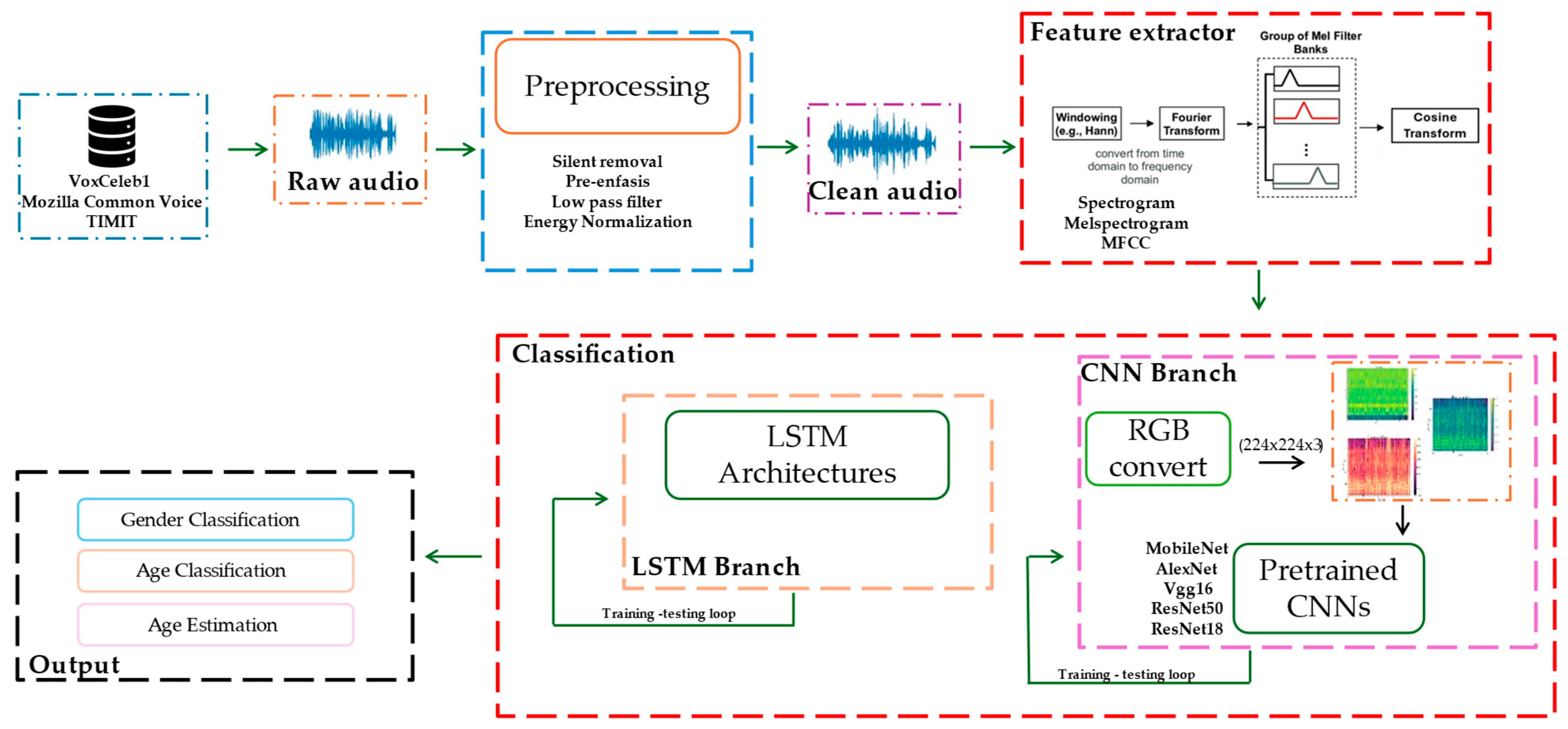
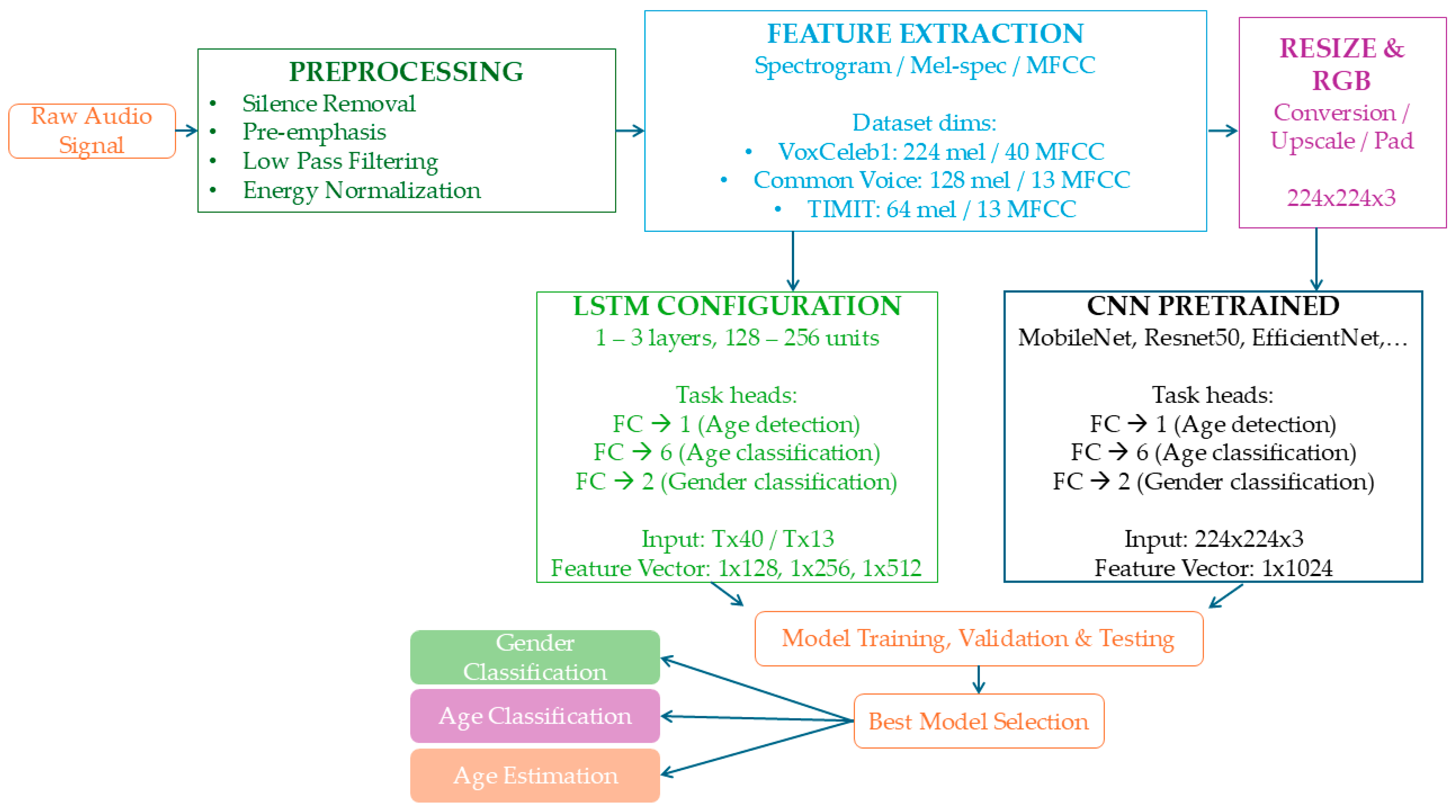
This study presents a framework for gender and age classification, as well as age estimation, based on speech signal analysis. The first stage involves preprocessing of the raw speech signal. Following preprocessing, feature extraction is performed by computing the spectrogram, Mel spectrogram, and MFCC. Finally, the classification stage leverages deep learning models, specifically CNNs and LSTM networks, to perform the tasks. We show an overview of our framework in Figure 1, which is explained in detail in the next sections.
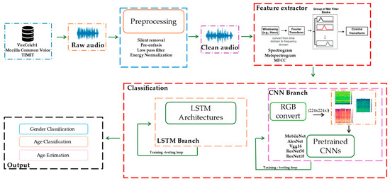
Figure 1.
Block diagram of proposed framework.
3.1. Preprocessing
Preprocessing raw audio enhances signal quality. This includes silence removal to retain only informative segments of speech, pre-emphasis filtering to boost high-frequency components, low-pass filtering to remove irrelevant noise, and energy normalization to standardize the amplitude levels across all samples.
3.1.1. Silence Removal
Speech signals often include silent segments, which can occur at the start, between words, or at the end of an utterance. Removing these non-speech portions helps to reduce both computational load and processing complexity. To enable more efficient analysis, these silent parts are typically discarded early in the processing pipeline. This is achieved by classifying each audio sample as either speech or silence based on the statistical characteristics of background noise.
First, the mean μ and variance σ of the voice signal x(t) are calculated by Equations (1) and (2).
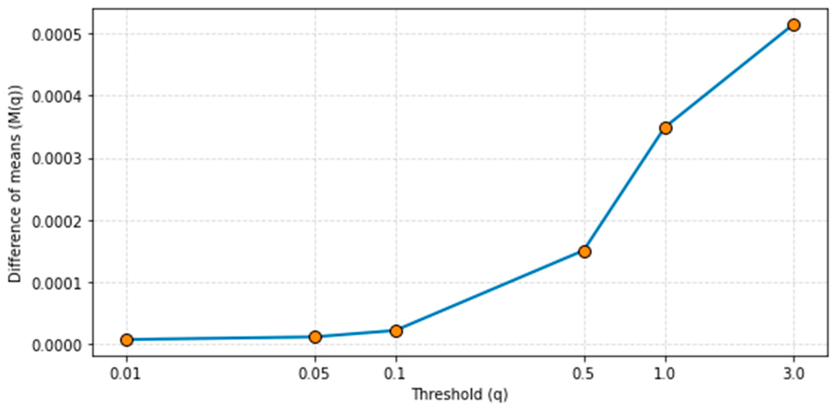
For each audio sample, if , then the sample is classified as speech; otherwise, it is considered as silence or an unvoiced segment [21], where is the threshold, whose value is determined so that the power spectral density (PSD) of the original and the silence-removed speech signal are almost the same, i.e., , where is frequency. Figure 2 shows an example of the silence removal process, showing the original speech signal and silence-removed signal in the time domain. We selected the threshold value based on Equation (3).
where is sampling frequency, and and are power spectral density of the original speech signal and silence-removed speech signal.
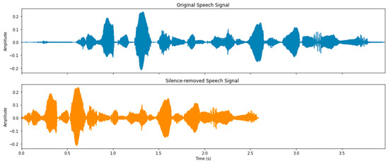
Figure 2.
Silence removal process.
We determined the threshold experimentally. In Figure 3 we show the results of these experiments. The optimal q is obtained for when is at a minimum but not zero. The experiments found that the optimal value for is between 0.05 and 0.1, we choose
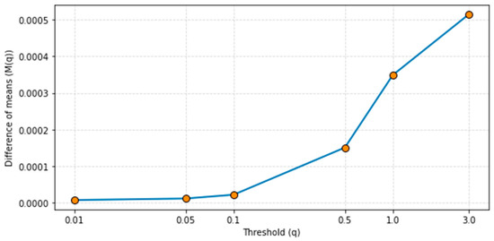
Figure 3.
Optimal threshold selection.
3.1.2. Pre-Emphasis
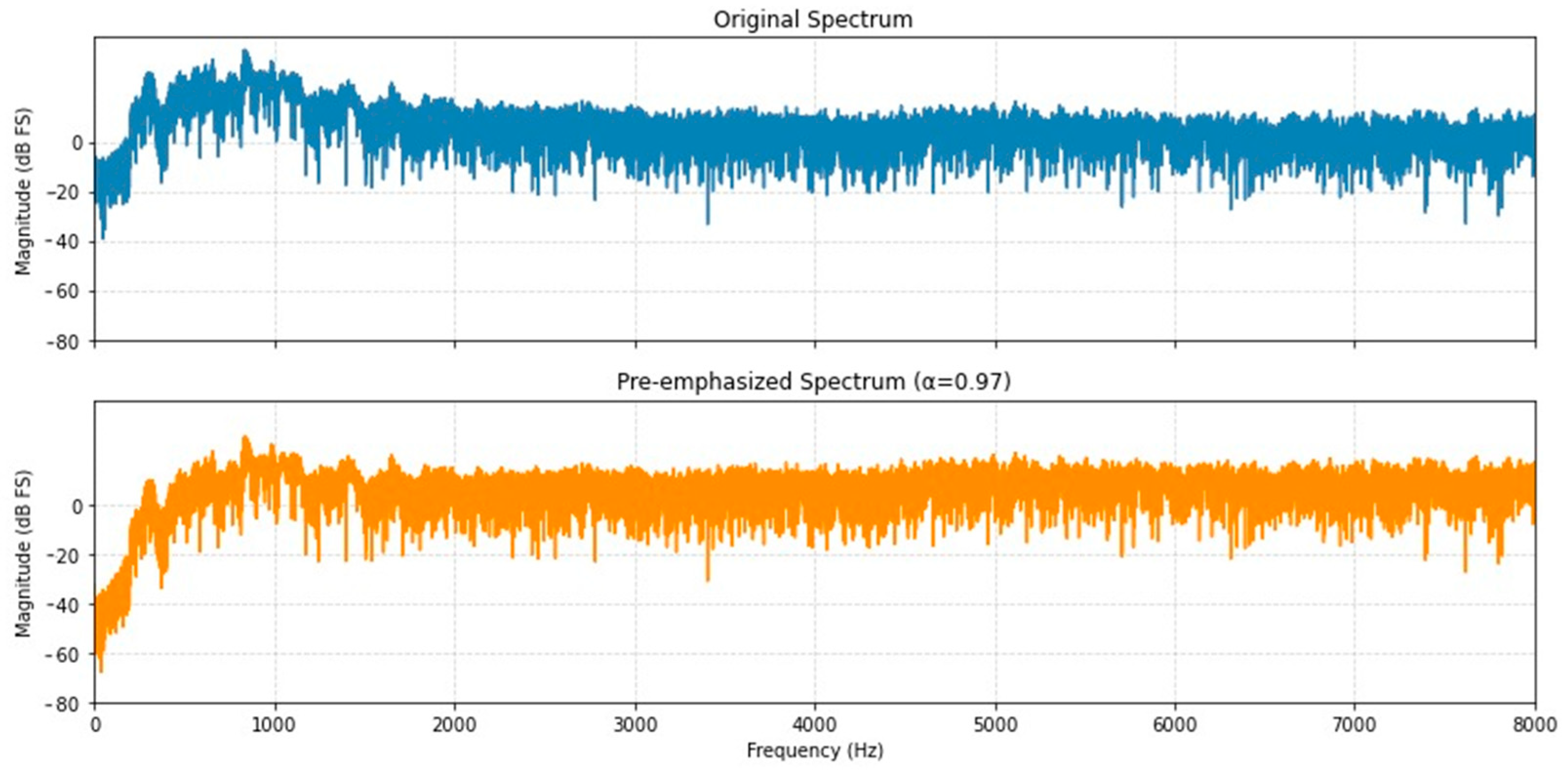
This technique is applied to counteract the natural spectral decay observed in the higher frequency range of spoken voice. As described by Ref. [21], the glottal source originating from the vocal folds introduces a spectral roll-off of approximately −12 dB per octave. In contrast, acoustic radiation at the lips contributes a spectral boost of around +6 dB per octave. As a result, when speech is recorded at a distance using a microphone, the captured signal exhibits an effective spectral slope of roughly −6 dB per octave relative to the actual vocal tract response. Pre-emphasis serves to suppress glottal influences and compensates for this attenuation, thereby enhancing spectral balance in the processed speech signal.
Pre-emphasis filtering, given by Equation (4), was applied to enhance the signal-to-noise ratio and the dynamic range of the recordings.
where is the sample signal at time , is the sample of the previous time step, is the pre-emphasis signal, and is the pre-emphasis coefficient, typically 0.97 [21,22]. This filter subtracts an attenuated version of the previous sample, enhancing rapid changes in the signal like high-frequency components. Figure 4 illustrates the pre-emphasis process.
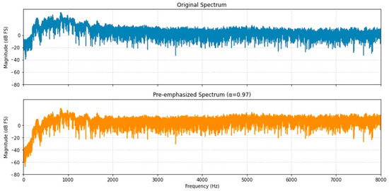
Figure 4.
Pre-emphasis filtering process.
3.1.3. Low-Pass Filtering
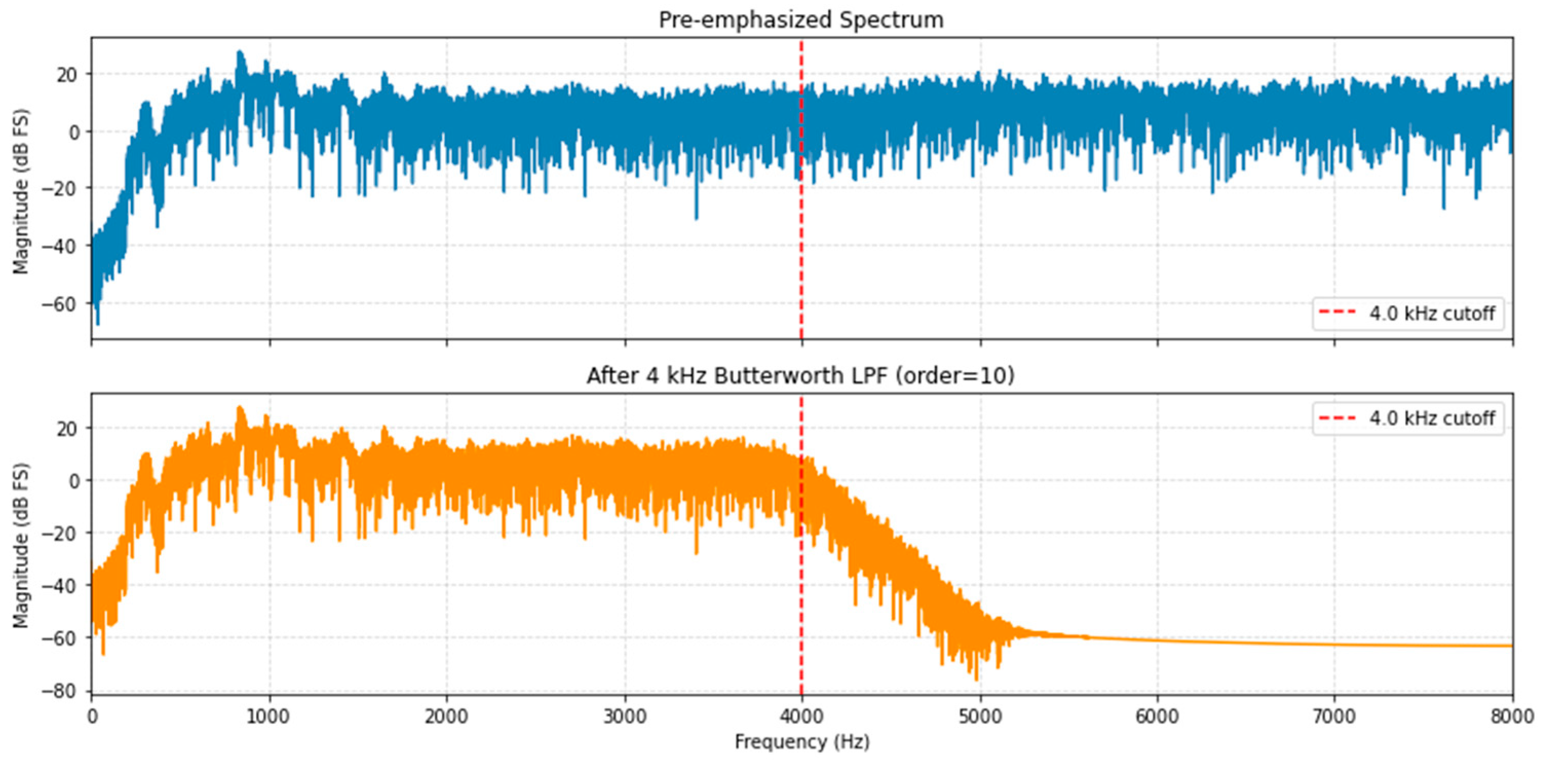
Low-pass filtering is an essential preprocessing step in speech processing applications due to the inherent frequency characteristics of speech signal, typically ranging from approximately 300 Hz to 4 kHz [23]. Speech signals are often recorded alongside irrelevant or undesired signals, such as high-frequency noise artifacts. Such noise is effectively reduced using low-pass filtering, which allows frequencies below a specified cutoff frequency to pass (passband), while attenuating frequencies above this threshold (stopband) [24]. Among various filter types, the Butterworth low-pass filter is particularly noted for its efficacy in acoustic voice analysis, owing to its smooth frequency response and maximally flat passband [25]. In this study, we employed a tenth-order Butterworth low-pass filter with a cutoff frequency of 4 kHz to effectively eliminate high-frequency noise components from the recorded speech signals. Figure 5 illustrates the implemented filtering process. We define the result signal as .

Figure 5.
Low-pass filtering.
3.1.4. Energy Normalization
According to the approach presented by [21,22,23], normalization is applied to speech signals to mitigate variations in amplitude, thereby facilitating meaningful comparisons across different signal instances. This process is defined by Equation (5), written as follows:
where is filtered signal, is number of samples, is the mean and is the standard deviation of . The resulting value, , represents the normalized version of the corresponding sample, ensuring that the signal is standardized with respect to its statistical distribution.
3.2. Feature Extraction
Spectral features were extracted to represent the voice signals for model training. Three types of features were computed: spectrograms, Mel spectrograms, and MFCCs. Spectrograms were generated by segmenting the signal into small blocks where window length is 25 ms with 10 ms of overlapping between consecutive frames, then a Hamming window is applied by Equation (6) [21] to smooth edges. where N is the number of samples in each frame.
Next, we compute the Short-Time Fourier Transform (STFT), providing a time-frequency representation of the signal’s energy. The Mel spectrograms were derived by applying a bank of triangular Mel filters to the spectrogram, which are non-linearly spaced, to mimic human auditory perception [26]. The central frequency of each Mel filter is given by Equation (7).
where is the lineal frequency and is the Mel frequency. Equation (8) represents the function of triangular filters.
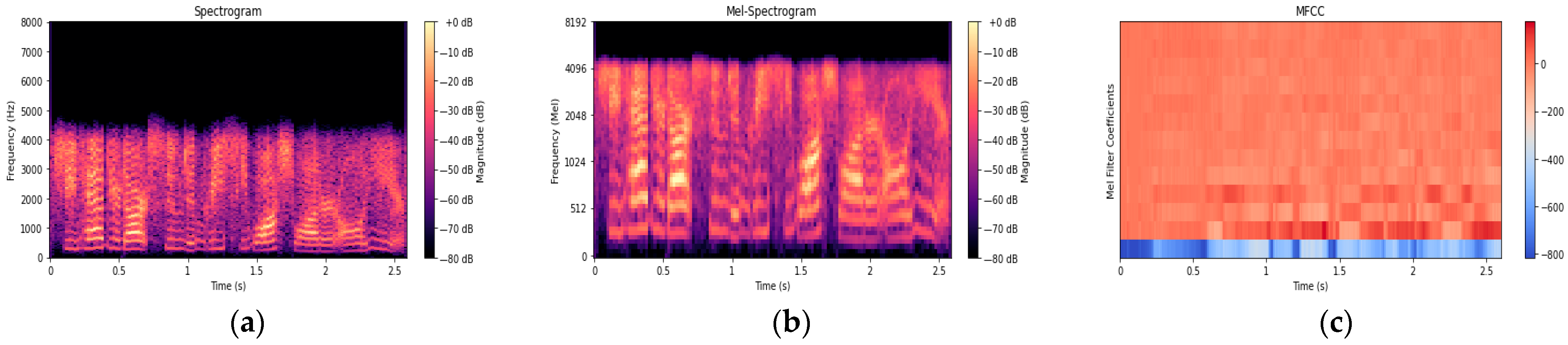
where , and represent the central frequency of the adjacent triangular filters, and represents the lineal frequency and the number of triangular filters. MFCCs were obtained by applying a Discrete Cosine Transform (DCT) to the log-energy output of the Mel filters, yielding a compact representation of the spectral envelope widely used in speech recognition and classification tasks [26,27]. Figure 6 shows the output of feature extraction from a sample speech signal.
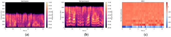
Figure 6.
Sampled of TIMIT speech signal feature vectors extraction. (a) Spectrogram, (b) Mel spectrogram, and (c) MFCC.
3.3. Classification
This section explains in detail the implementation of our proposal and describes the feature selection and training process below.
3.3.1. Feature Selection for Classifiers
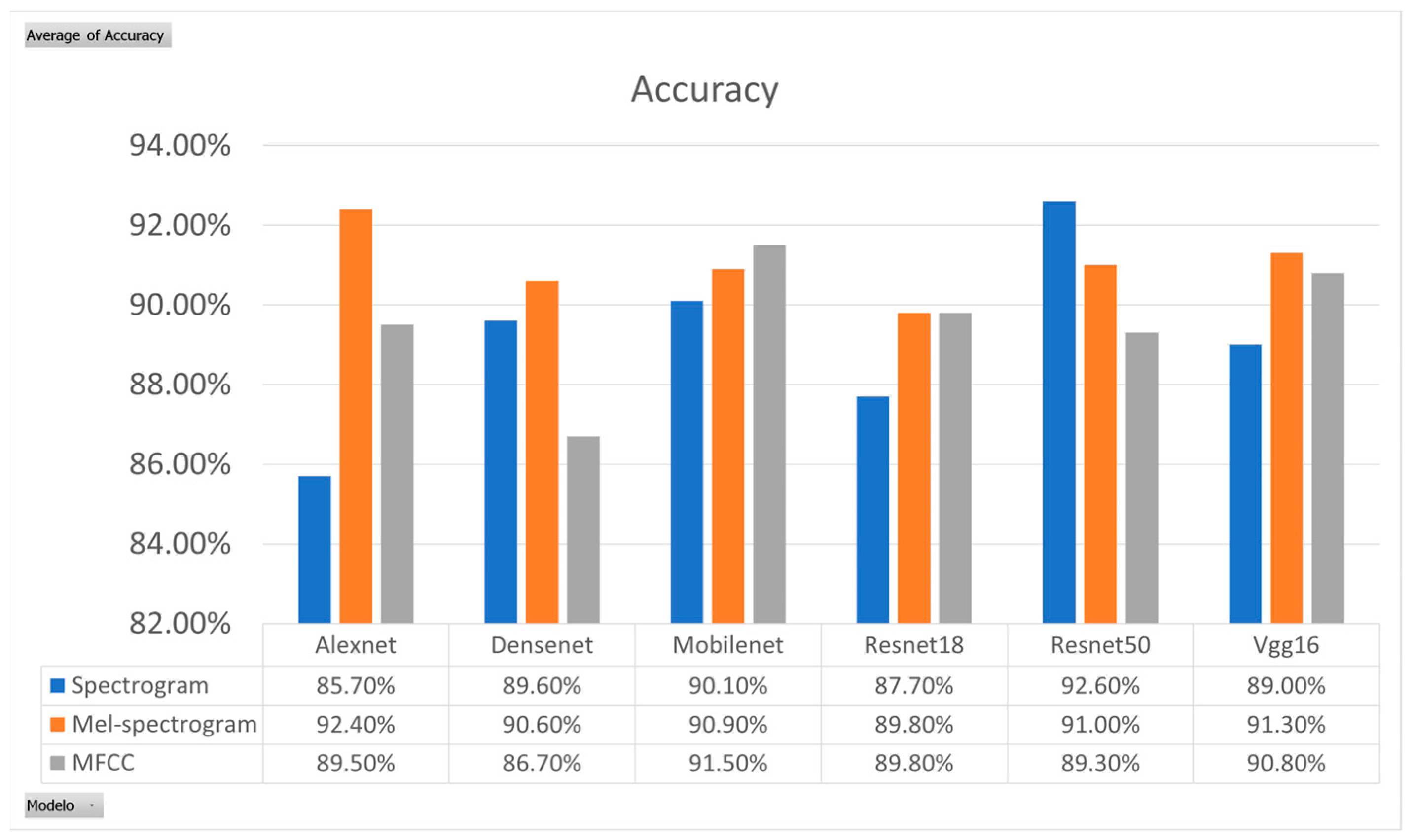
To determine the most suitable features for our system, training and validation experiments were conducted using a smaller dataset extracted from VoxCeleb1, which is the most challenged for its in-the-wild characteristic. This subset is called Subset 1, consisting of 5000 audio samples for training and 500 for validation. Various pre-trained CNN models and LSTM configurations were evaluated in this stage. For CNNs, the three features’ vectors spectrogram, Mel spectrogram, and MFCC were converted into 224 × 224 RGB images as shown to ensure compatibility with the input requirements of the CNN pre-trained models.
Experimental results shown in Figure 7 indicate that Mel spectrograms yielded the best performance for CNN model training, while MFCCs have demonstrated higher effectiveness than Mel spectrograms and spectrograms for LSTM [28]. So, we use the Mel spectrogram for CNNs and MFCC for LSTM in our experiments.

Figure 7.
Experimental results for features vectors.
The dimensionality of the Mel spectrogram was adapted to each corpus. VoxCeleb1 recordings, which contain background noise and speaker overlap, were encoded with 224 Mel coefficients [29] to preserve fine-grained spectral detail. Mozilla Common Voice, whose utterances are cleaner, required only 128 coefficients, while the comparatively noise-free TIMIT corpus was adequately represented with 64 coefficients. Table 1 summarized the number of coefficients used for different datasets. Mel coefficients were used to obtain RGB images for introducing into CNN models and MFCC for LSTM models.

Table 1.
Feature extraction parameters.
3.3.2. Training of Classifiers
Each corpus was processed independently using a stratified 80–20% train–test split. Optimization employed Adam [30] with a Reduce-on-Plateau [31] scheduler (initial learning rate = 1 × 10⁻³, minimum = 1 × 10⁻⁶, patience = 3, reduction factor = 0.5). Early stopping [32] (patience = 15) and best-checkpoint saving were enabled. Generalization was promoted through L2 weight decay [33] (1 × 10⁻⁴) and dropout [34] (p = 0.5). Cross-Entropy Loss Function [35] was utilized for classification tasks and MAE (L1 Loss) [36] for estimation tasks.
The training process was divided into the following two stages:
- Stage 1—Model Selection: Transfer learning was applied to various pre-trained CNN models, and multiple LSTM configurations were trained on Subset 1. The top three CNN models and the best LSTM configuration were selected based on classification accuracy for gender and age classification or MAE for age estimation.
- Stage 2—Fine-Tuning and Full Training: The selected CNN models underwent fine-tuning, and the best LSTM configuration was trained on the complete datasets to optimize the performance. This two-stage approach leverages the strengths of transfer learning for CNNs and systematic hyperparameter tuning for LSTMs, ensuring robust adaptation to the gender classification and age estimation tasks.
Figure 8 presents a graphical overview of the complete process from the raw signal processing to pre-trained experts obtaining. Details of preprocessing and feature extraction were given in Section 3.1 and Section 3.2; additional details are given in Section 3.3.
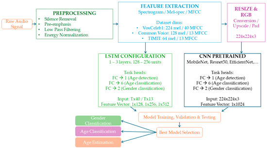
Figure 8.
Pipeline of our proposal.
First Stage
The primary objective of this section is to perform a series of training and validation experiments to identify optimal models for voice-based classification and regression tasks. A reduced dataset, referred to as Subset 1, was employed to evaluate model performance, with model selection based on the highest accuracy for classification tasks and the lowest MAE for regression tasks. The evaluation process involved several pre-trained CNN architectures over ImageNet [37], a large dataset for image classification, including AlexNet [38], ResNet18, ResNet50 [39], EfficientNet [40], DenseNet [41], VGG16 [42], and MobileNet [43]. These models were selected as starting points due to their proven effectiveness in image-based tasks, and transfer learning techniques were applied to adapt them to our specific problem.
Transfer learning, as described by Ref. [44], leverages a model pre-trained on a large-scale dataset. This study used pre-trained CNNs with ImageNet and fine-tuned them for a target task by retraining specific layers with domain-specific data. In this study, the last convolutional layer of each CNN model was retrained. The output layer was modified to match the requirements of each task: for gender classification, the output layer was adjusted to two units for binary classification; for age classification, to six units, corresponding to six age groups; and for age estimation, it was configured to a single unit. This approach ensures that the models retain general feature extraction capabilities from ImageNet while adapting to the spectral characteristics of voice data, represented as Mel spectrogram images.
For LSTM networks, a series of configurations were trained and evaluated to determine the optimal architecture. The configurations varied in the number of units per layer (1, 2, or 3) and the number of hidden units (128, 256, or 512). Unlike the CNN models, the LSTM networks were trained directly on MFCCs, which are widely used for capturing temporal and spectral features in speech signals. MFCCs were selected due to their effectiveness in representing the short-term power spectrum of speech, making them suitable for sequential modeling with LSTMs.
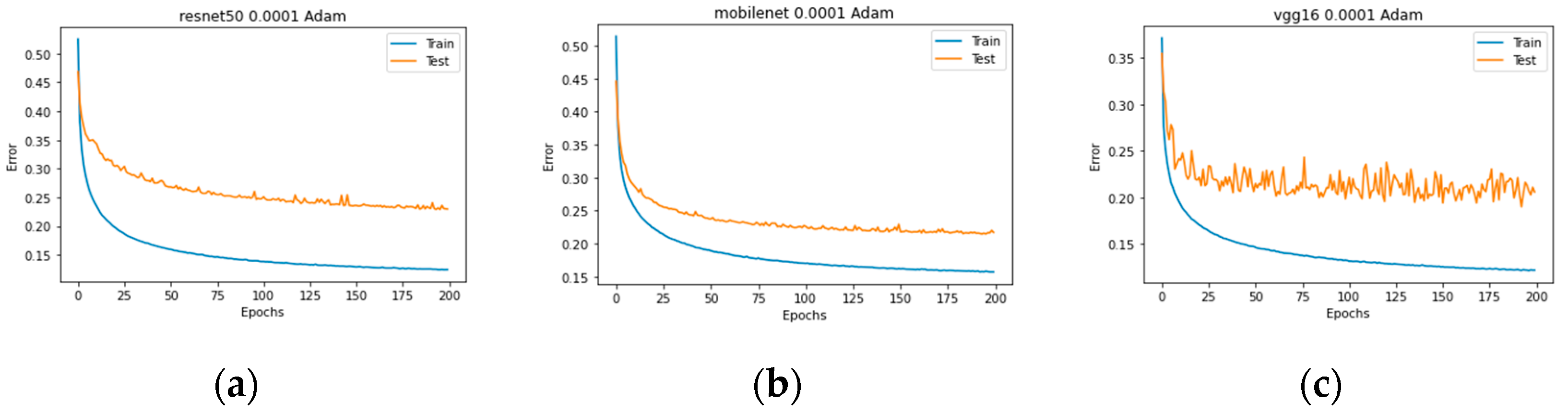
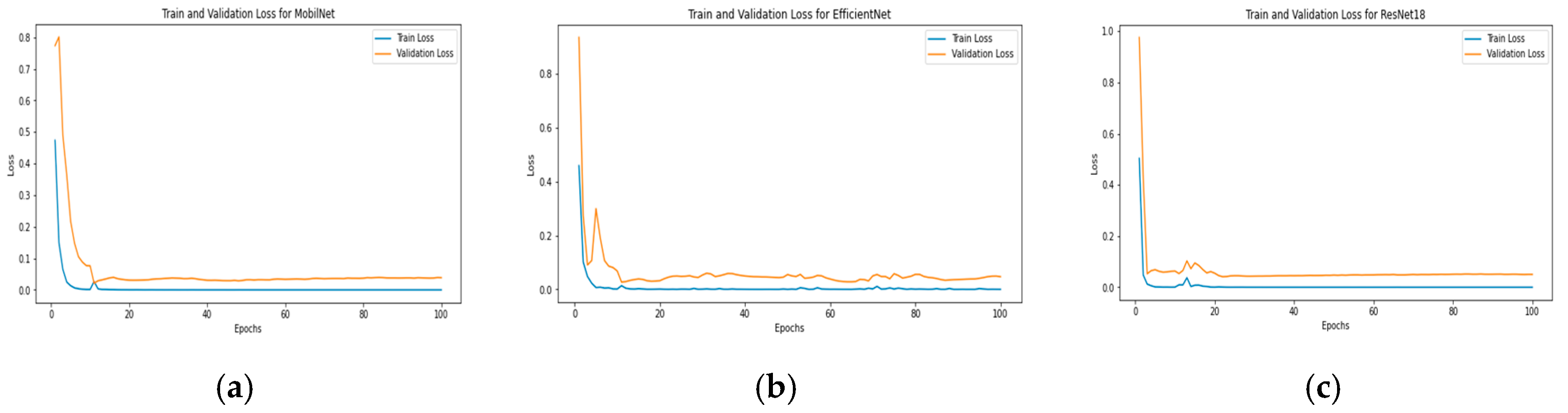
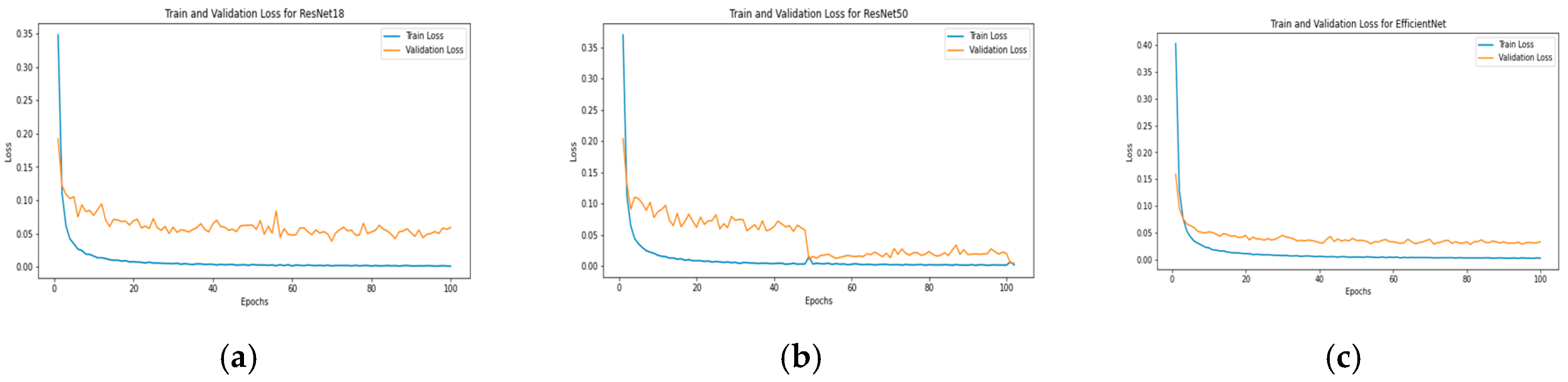
In the initial evaluation stage, experiments were conducted across three benchmark datasets. For VoxCeleb1, the top-performing models were ResNet50, MobileNet, and VGG16, demonstrating robust generalization across diverse speakers. On the Mozilla Common Voice dataset, ResNet18, ResNet50, and EfficientNet achieved the highest average accuracies, reflecting their ability to handle large-scale, crowdsourced voice data. Similarly, for the TIMIT dataset, MobileNet, ResNet18, and EfficientNet emerged as the best performers, likely due to their efficiency in extracting features from the controlled, phonetically balanced recordings in TIMIT. These results highlight the variability in model performance across datasets, underscoring the importance of dataset-specific characteristics in model selection. Figure 9, Figure 10 and Figure 11 illustrate the training process.
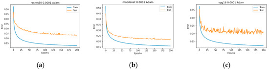
Figure 9.
Training process Stage 1 VoxCeleb1: (a) ResNet50, (b) MobileNet, and (c) Vgg16.
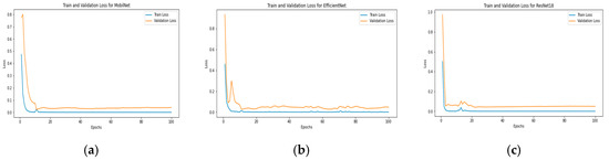
Figure 10.
Training process Stage 1 Mozilla Common Voice: (a) ResNet18, (b) ResNet50, and (c) EfficientNet.
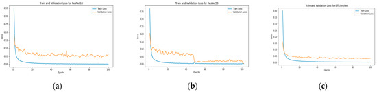
Figure 11.
Training process Stage 1 TIMIT: (a) MobileNet, (b) EfficientNet, and (c) ResNet50.
Second Stage
In this phase, fine-tuning was performed on the pre-selected models identified in the previous stage for each dataset: VGG16, MobileNet, EfficientNet, ResNet50, and ResNet18. Fine-tuning, a key strategy in transfer learning, involves adapting a pre-trained model to a new task by selectively updating a subset of its layers while preserving the knowledge encoded in earlier layers. To achieve this, the weights of the initial layers were frozen to retain the general feature extraction capabilities learned from ImageNet, while the later layers were retrained to adapt to the spectral characteristics of our voice datasets, represented as Mel spectrogram images.
This fine-tuning approach aligns with established practices in transfer learning, where freezing earlier layers preserves low-level features (e.g., edges, textures) while retraining later layers allows the model to learn task-specific, high-level features [45]. By focusing retraining on the final blocks, we ensure computational efficiency while enabling the models to adapt effectively to the voice classification and regression tasks. Appendix A resumes the frozen and the retrained layers of each CNNs used in this stage.
We conducted all DNN processing in the PyTorch Library version 2.2.1. The training sessions were carried out on a computer with the following hardware components:
- Graphics Card: NVIDIA GeForce RTX 3070 Ti, NVIDIA, Santa Clara, CA, USA.
- Graphics Clock: 1770 MHz.
- Total Available Memory: 24,527 MB.
- Host: Ryzen 7 3700x 8-core CPU at 3.60 GHz, 32 GB RAM, AMD, Santa Clara, CA, USA.
4. Results and Discussion
In this section, the first three datasets used for evaluation are described in detail, and then we expose the results achieved in our research. We show some metrics like accuracy, confusion matrix, and MAE. Additionally, we expose the detailed features of used datasets.
4.1. Datasets
This study leverages three well-established datasets for voice-based classification tasks: VoxCeleb 1, Mozilla Common Voice, and TIMIT. These datasets were selected for their diversity in recording conditions, speaker demographics, and linguistic coverage, enabling a comprehensive evaluation of the proposed models across varied scenarios.
VoxCeleb 1 is a large-scale dataset designed for speaker recognition research, comprising 145,265 audio segments from 1251 speakers of diverse geographical and demographic backgrounds [46]. The recordings are captured in uncontrolled environments, introducing environmental noise that poses challenges for voice signal processing and classification. The characteristics “in the wild” is the motivation to utilize it in this approach. The sampling rate of this dataset is 16 kHz.
The Mozilla Common Voice dataset is a widely used, multilingual collection of transcribed speech, specifically curated for ASP research [47]. It includes recordings in over 60 languages, with demographic metadata such as age, gender, and accent, making it ideal for tasks requiring linguistic and demographic diversity. In this study, we utilized Common Voice Corpus version 17.0. The diversity of accents and amount of available data make this dataset ideal for the tasks we conducted. The sampling rate of this dataset is 44.1 kHz.
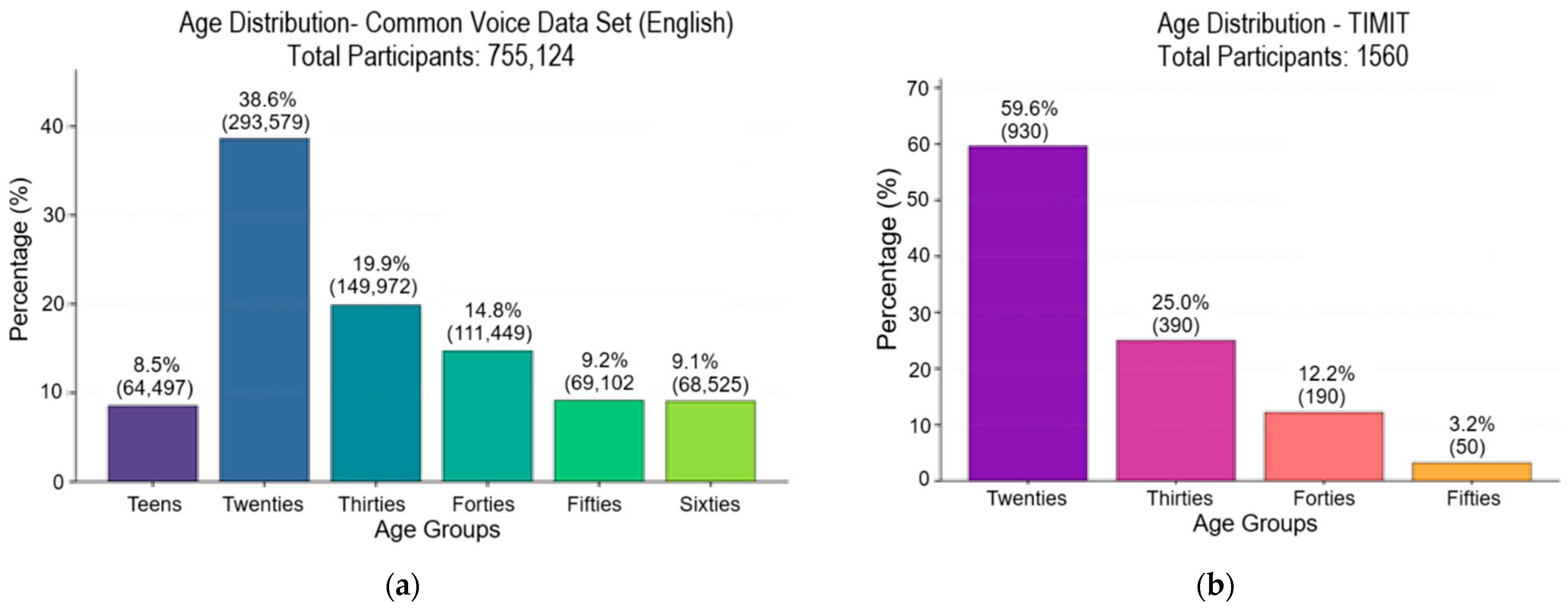
The TIMIT Acoustic-Phonetic Continuous Speech Corpus is a standard benchmark for evaluating ASP systems [48]. It contains recordings from 630 speakers across eight major dialect regions of the United States, with each speaker reading ten phonetically rich sentences. TIMIT includes a gender distribution of 438 male and 192 female speakers. While the exact age distribution is not specified. The uses of this dataset in many studies and its availability and age-labeled data make this dataset a complement to develop our study. The sampling frequency is 16 kHz. Table 2 illustrates the datasets composition and characteristics, and Figure 12 show the age distribution of the Mozilla Common Voice and TIMIT datasets.
Table 2.
Datasets composition and characteristics.

Figure 12.
Age distribution: (a) Mozilla Common Voice and (b) VoxCeleb1.
Audio from the VoxCeleb1 and TIMIT corpora was processed at 16 kHz because this rate, native to both datasets, captures the 0–8 kHz speech band while reducing storage and compute. Common Voice recordings, originally distributed at 44.1 kHz, were down-sampled to 22.05 kHz—exactly half of the 44.1 kHz consumer-audio family—so as to preserve spectral content up to 11.025 kHz. Moreover, empirical studies show that 22.05 kHz yields negligible intelligibility loss relative to higher rates while halving bandwidth, making it a pragmatic choice for wide-band speech pipelines. Consequently, the combined use of 16 kHz for recognition and 22.05 kHz for synthesis offers a widely endorsed balance between perceptual fidelity and resource efficiency in modern speech-technology research [49].
4.2. Results
Firstly, we present the results of experts for the VoxCeleb1 Dataset. Table 3 and Figure 13 show the accuracy for the three best results for CNN and the confusion matrix.
Table 3.
Results of CNN over VoxCeleb1.

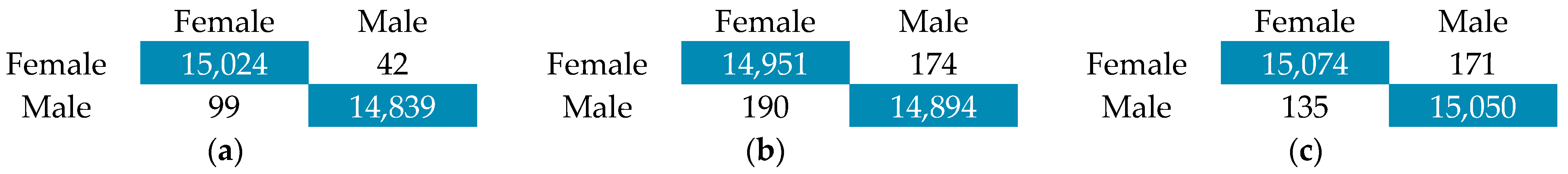
Figure 13.
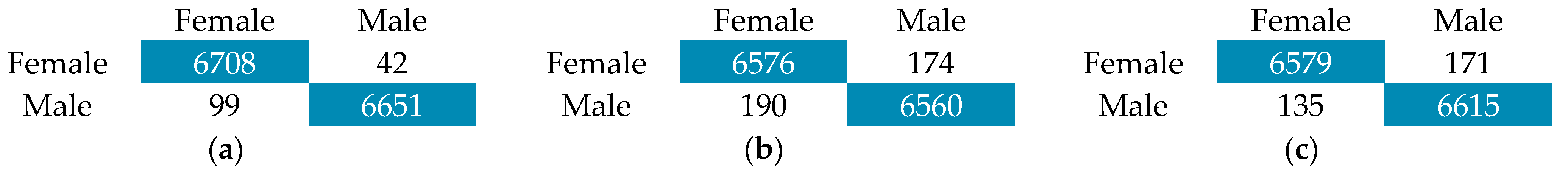
Confusion matrix VoxCeleb1 for (a) MobileNet; (b) VGG16; (c) ResNet50.
The results clearly show that the better model from CNN is MobileNet with a 98.96% accuracy. The confusion matrix shows that the gender classification model performs exceptionally well, with an overall accuracy of 98.96%. It correctly classified 6708 female and 6651 male samples. Only 42 female samples were misclassified as male, and 99 male samples were misclassified as female. These results indicate that the model has both high precision and recall, making it highly reliable for gender classification based on voice features.
Table 4 shows the accuracies for the three best configurations of LSTM networks.
Table 4.
Results of LSTM over VoxCeleb1.
Table 4 presents the classification accuracy obtained by different LSTM configurations trained on 40 MFCC features for 100 epochs. The best result, 97.68% accuracy, was achieved using an architecture with three LSTM layers and 512 hidden units per layer. Other configurations, such as two layers with 256 hidden units or three layers with 256 units, yielded slightly lower accuracies of 97.50% and 97.52%, respectively. These findings suggest that increasing the hidden layer size contributes more significantly to performance improvement than increasing the number of stacked layers.
Now we present the results for experts on Mozilla Common Voice. In this case we evaluate the performance for gender and age classification tasks, as we mentioned before. We conducted these experiments for six classes for age and two classes for gender. Table 5 summarizes the results for CNN age and gender classification. Figure 14 shows the confusion matrix for each model.
Table 5.
Accuracy of CNN over Mozilla Common Voice.
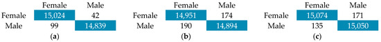
Figure 14.
Confusion matrix Common Voice for (a) ResNet18; (b) ResNet50; (c) EfficientNet.
For gender classification, all models achieved high accuracy, with EfficientNet leading at 99.82%. In age classification, ResNet50 performed with the best accuracy at 99.86%. These results highlight the effectiveness of CNNs in capturing spectral patterns, with deeper architectures like ResNet50 showing slight advantages for age classification.
For LSTM, Table 6 summarizes the results for age and gender.
Table 6.
Accuracy of LSTM over Mozilla Common Voice.
For gender classification, CNN models achieved high accuracy, with EfficientNet leading at 99.82%. In age classification, ResNet50 performed the best accuracy at 99.86%. These results highlight the effectiveness of CNNs in capturing spectral patterns, with deeper architectures like ResNet50 showing slight advantages for age classification.
Analyzing the results for LSTM, for gender classification, accuracies ranged from 93.63% to 97.67%, with the best performance (97.67%) achieved using 512 units and 3 layers. In age classification, accuracy ranged from 98.55% to 98.81%, with the same configuration yielding the highest accuracy (98.81%). Increasing the number of layers and units improved performance, though the results remained below those of CNNs.
For the TIMIT corpus, the results are resumed in Table 7, and Figure 15 shows the confusion matrix for each result. For gender classification there are two models with the same result: ResNet50 and MobileNet, which obtained a 99.23% accuracy. In the case of age estimation, the most efficient model is MobileNet, with 5.35 years of MAE, which is significant compared with the state-of-the-art.
Table 7.
Summarizes the results for CNN using TMIT dataset.
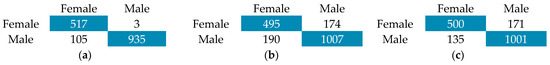
Figure 15.
Confusion matrix TIMIT for (a) MobileNet; (b) AlexNet; (c) ResNet50.
Results for LSTM over the TIMIT corpus are shown in Table 8. The most relevant is a configuration of 512 hidden neurons and two layers of length with 5.45 years of MAE, a competitive result.
Table 8.
Age estimation and gender classification accuracies using LSTM over the TIMIT dataset.
CNN experts consistently outperformed LSTMs in both tasks, achieving accuracy above 99% compared to LSTMs’ maximum of 97.67% (gender) and 98.81% (age). This gap likely stems from the Mel spectrogram representations used by CNNs, which better capture spectral patterns, versus the sequential MFCC inputs for LSTMs. The findings suggest that CNNs are more suited for these voice classification tasks, though LSTMs still offer competitive performance, particularly with optimized configurations. In Table 9 we make a summary of the main results obtained by distributing over three employed datasets.
Table 9.
Experimental results–classification accuracies (%) with network model. MCV means Mozilla Common Voice Dataset.
Table 9 demonstrates that the proposed models achieve excellent in-domain performance, with gender and age classification accuracies exceeding 98%, peaking at 99.82% for gender (EfficientNet on MCV) and 99.86% for age (ResNet50 on MCV). Based on our experimental results, we make a comparison between related work and our proposal. Table 10 shows the comparison.
Table 10.
Comparison of proposed method with related works.
Table 10 and Figure 16 show a comparison with the state-of-the-art baseline and our proposal. The references for comparison are shown in the table, and the figure represents in visual form this comparison.
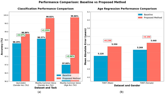
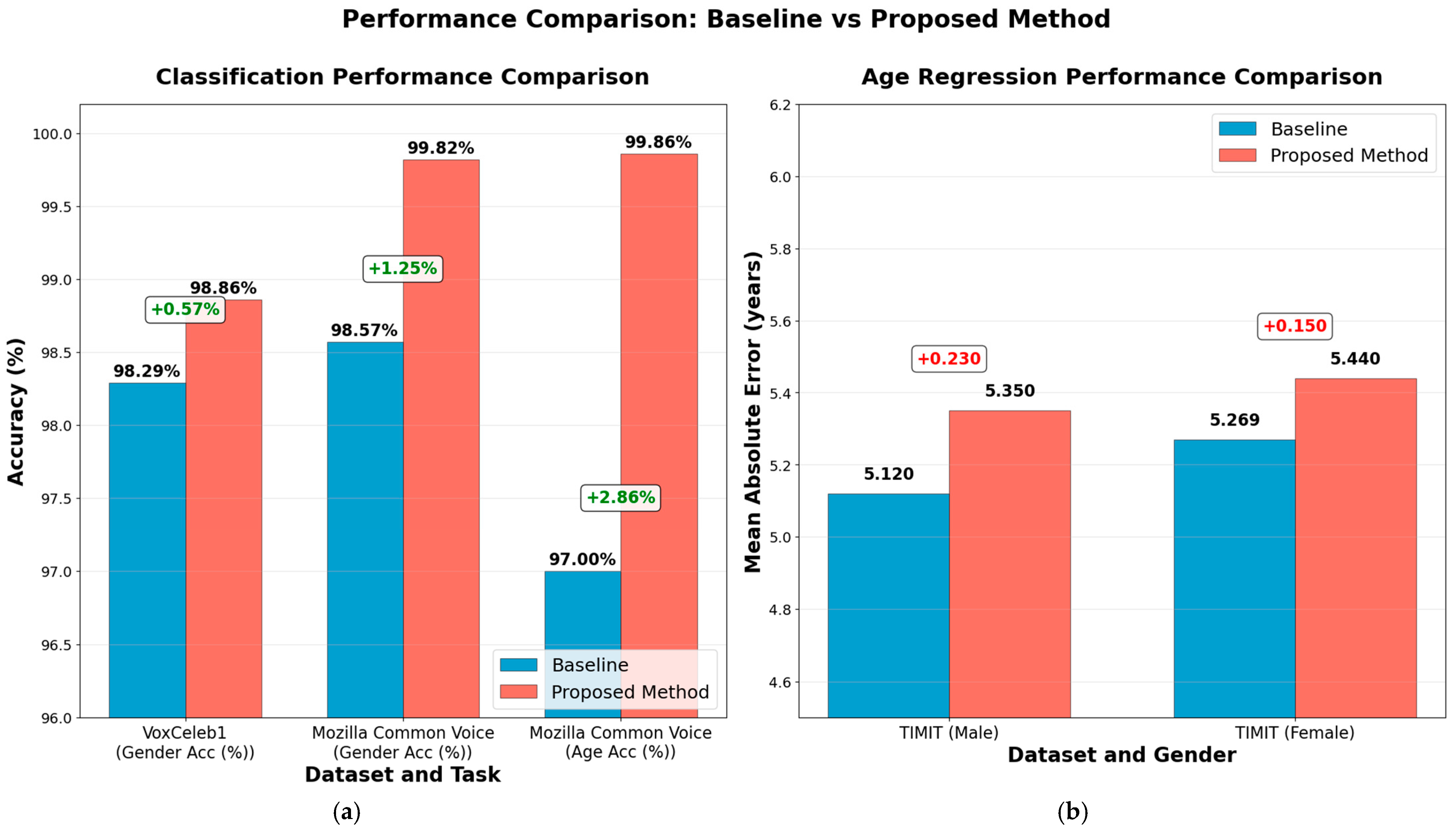
Figure 16.
Performance comparison: (a) classification tasks and (b) regression task.
Our proposed approach delivers substantial gains in gender and age classification on large, real-world speech datasets. On VoxCeleb1, gender-classification accuracy rises from 98.29% to 98.86% (Δ + 0.57), and on Mozilla Common Voice, it jumps from 98.57% to 99.82% for gender (Δ + 1.25) and from 97.00% to 99.86% for age (Δ + 2.86), effectively driving error rates to near zero on this challenging, in-the-wild corpus.
In contrast, age-estimation MAE on the smaller, more controlled TIMIT dataset increases slightly from 5.12 to 5.35 years for males (Δ + 0.23) and from 5.29 to 5.44 years for females (Δ + 0.15), indicating a minor trade-off in fine-grained regression performance. Overall, the method sets new state-of-the-art benchmarks in classification while remaining competitive in age estimation.
As shown in Table 10, incorporating audio preprocessing consistently enhances performance across datasets, underscoring the importance of preprocessing steps to effectively capture discriminative audio features.
5. Conclusions and Future Work
This study presents a comprehensive evaluation of deep learning models—specifically CNNs and LSTMs—for gender and age classification, as well as age estimation, from voice signals. Across three benchmark datasets, VoxCeleb1, Mozilla Common Voice, and TIMIT, the proposed approach achieves high in-domain performance.
We conclude our work on the following five points:
- Improving results using fine preprocessing.
We propose a comprehensive preprocessing and feature extraction methodology aimed at addressing existing limitations in current approaches. By systematically evaluating multiple feature configurations, we validate the effectiveness and applicability of our proposed method. Our approach not only facilitates improved data representation but also demonstrably enhances overall performance metrics, as evidenced by experimental validation.
- CNN/LSTM pipeline generalizes across diverse corpora without hyperparameter retuning.
Using an identical training recipe on VoxCeleb1, Common Voice, and TIMIT, all models maintained greater than 98% accuracy across gender and age group, or less than 5.4 years in MAE. This shows that network design—not corpus-specific tweaking—is the principal driver of performance.
- Model capacity should match corpus scale.
EfficientNet and ResNet50 delivered the best accuracies on the two large-scale datasets (VoxCeleb1, Common Voice), whereas the lightweight MobileNet-V2 achieved the lowest MAE on the small TIMIT corpus. This confirms that over-parameterized models can overfit limited data, while compact architectures excel in low-resource settings.
- Front-end choice must fit the architecture.
A set of comparative tests showed that CNNs improve by +1.3 to +1.8 percentage points when they take Mel spectrograms instead of MFCC vectors; this margin was consistent across all three corpora. In contrast, LSTMs gained only a modest increase of approximately +0.4 pp when using MFCCs, whose cepstral coefficients compress the spectral envelope and favor recurrent temporal modeling—an outcome aligned with standard practice in the literature. Although not an exhaustive ablation, these results support the rule of thumb: use high-resolution 2D spectral images for convolutional networks and compact MFCC trajectories for recurrent networks, aligning spectral resolution with the receptive-field size and shape of the model.
- Performance improvements over prior art is statistically significant
The proposed pipeline surpasses the previous state of the art by +1.25 pp (gender-MCV), +2.86 pp (age-MCV) and +0.57 pp (gender-VoxCeleb1).
As future work, we propose exploring domain adaptation techniques and data augmentation strategies to enhance model robustness. In domain adaptation, we consider that the proposed system, trained for the English language, will adapt to Mexican Spanish or Cuban Spanish. The primary challenge for this adaptation is the lack of sufficient labeled data for training. As domain adaptation techniques, pseudo-labeling and teacher-student techniques can be applied to data with labels. Both techniques generate a large enough dataset from a small dataset. The data augmentation technique involves artificially generating data by applying several audio processing techniques to real data, such as speech perturbation, pitch shifting, and time stretching. These techniques can also be applied to a small dataset, such as the TIMIT dataset, to enhance classification and estimation accuracy. The pseudocodes of the proposed method are provided in Appendix B for better comprehension.
Author Contributions
Conceptualization, J.J.-C.; data curation, J.J.-C.; formal analysis, L.H.-G.; investigation, J.J.-C., M.N., H.P.-M. and L.H.-G.; methodology, M.N.; software, J.J.-C.; validation, M.N.; visualization, H.P.-M.; writing—original draft, J.J.-C.; writing—review and editing, M.N. and H.P.-M. All authors have read and agreed to the published version of the manuscript.
Funding
This research received no external funding.
Institutional Review Board Statement
Not applicable.
Informed Consent Statement
Not applicable.
Data Availability Statement
The data presented in this study are openly available in VoxCeleb1 at [13], the Common Voice dataset at [14], and the TIMIT dataset [15].
Conflicts of Interest
The authors declare no conflicts of interest.
Appendix A
Table A1 summarizes the fine-tuning strategy for each convolutional backbone. For all networks the lower-level feature extractors were kept intact, while the deeper semantic blocks and the final classifier were updated. Concretely, VGG-16 was fine-tuned from block 4 onward, both ResNet variants from conv4_x onward, MobileNet V2 from block 16 onward, and EfficientNet-B0 from stage 6 onward. This balanced scheme preserves generic visual features, shortens training time, and mitigates overfitting while still giving the model capacity to adapt to the target domain.
Table A1.
Fine-tuning CNN models.
Table A1.
Fine-tuning CNN models.
| Model | Frozen Layers (Blocks) | Retrained Layers (Blocks) |
|---|---|---|
| VGG16 | Blocks 1–3 (conv1_1—conv3_3) | Blocks 4 and 5 (conv4_1—conv5_3) |
| ResNet50 | Stem conv1 + Layer1 (conv2_x) + Layer2 (conv3_x) | Layer3 (conv4_x) and Layer4 (conv5_x) |
| ResNet18 | Stem conv1 + Layer1 (conv2_x) + Layer2 (conv3_x) | Layer3 (conv4_x) and Layer4 (conv5_x) |
| MobileNetV2 | Conv2dNormActivation (block 0) + Inverted Residual blocks 1–15 | Inverted Residual blocks 16 and 17 + Classification head |
| EfficientNet-B0 | Stem conv + Stages 1–5 (MBConv1/MBConv6) | Stages 6 and 7 (MBConv6) + Head |
Appendix B
This appendix contains complete pseudocode that describes the pipeline used in our proposal to improve comprehension and facilitate replication.
- 0.
- Constants & Conventions
DATASETS = {
  "VoxCeleb1":  {fs_in:16_000, fs_proc:16_000, n_mels:224, n_mfcc:40},
  "CommonVoice": {fs_in:44_100, fs_proc:22_050, n_mels:128, n_mfcc:13},
  "TIMIT":       {fs_in:16_000, fs_proc:16_000, n_mels:64, n_mfcc:13}
       }
WINDOW_LEN = 25 ms
WINDOW_STEP = 10 ms
IMG_SIZE   = 224×224×3
OPTIM      = Adam(lr=1e-3, weight_decay=1e-4)
SCHED      = ReduceOnPlateau(factor=0.5, patience=3, min_lr=1e-6)
EARLY_STOP = patience 15
DROPOUT    = 0.5
- 1.
-
Main Flow
for corpus in DATASETS:
   train_set, test_set = stratify(corpus, split=0.8)
   cnn_models   = train_CNN_stage1(train_set, corpus)
   lstm_model   = train_LSTM_stage1(train_set, corpus)

   top_cnns     = select_top3(cnn_models, metric="accuracy-or-MAE")
   top_lstm     = select_top1(lstm_model, metric="accuracy-or-MAE")

   final_models = fine_tune_stage2(top_cnns, top_lstm, train_set, corpus)

   evaluate(final_models, test_set, corpus)
   save(final_models, path="checkpoints/"+corpus)
- 2.
-
Audio Preprocessing
def preprocess(wav, fs_in, fs_proc):
    # 2.1 Resampling
    wav = resample(wav, fs_in, fs_proc)

    # 2.2 Silence removal
    μ, σ = mean_variance(wav)
    threshold = q # choose q ∈[0.05,0.1]
    wav = discard_samples(|wav|2 < threshold)

    # 2.3 Pre–emphasis
    wav = pre_emphasis_filter(wav, α=0.97)

    # 2.4 10th-order Butterworth low-pass, fc=4 kHz
    wav = butter_lowpass(wav, order=10, fc=4_000, fs=fs_proc)

    # 2.5 Energy Normalization
    wav = (wav-μ)/σ
    return wav
- 3.
-
Feature Extraction
def extract_features(wav, corpus):
    # 3.1 Frame segmentation + Hamming window
    frames = window(wav, WINDOW_LEN, WINDOW_STEP)

    # 3.2 Power spectrogram (STFT)
    spec = |STFT(frames)|2

    # 3.3 Mel spectrogram
    mel = apply_mel_bank(spec, n_mels=DATASETS[corpus].n_mels)

    # 3.4 MFCC
    mfcc = DCT(log(mel))[:DATASETS[corpus].n_mfcc]

    # 3.5 Prepare for CNN
    img = resize_to_RGB(mel, target=IMG_SIZE)

    return img, mfcc
- 4.
-
Training—Stage 1 (model selection)
def train_CNN_stage1(data, corpus):
    SUBSET = sample(data, n_train=5_000, n_val=500)  # VoxCeleb1 “Subset 1”
    ARCHS = [AlexNet, VGG16, ResNet18, ResNet50, DenseNet, EfficientNet, MobileNet]
    results = {}
    for arch in ARCHS:
       net = load_pretrained(arch, "ImageNet")
       freeze_base(net)
       replace_head(net, task_output)  # 2-class, 6-class or 1-reg
       metrics = train(net, SUBSET.img, labels, OPTIM, SCHED, EARLY_STOP, DROPOUT)
       results[arch] = metrics
  return results

def train_LSTM_stage1(data, corpus):
    CONFIGS = combinations(layers=[1,2,3], hidden=[128,256,512])
    results = {}
    for layers, hidden in CONFIGS:
        net = LSTM(input_dim=DATASETS[corpus].n_mfcc,
                 hidden_dim=hidden,
                 num_layers=layers, dropout=DROPOUT)
        metrics = train(net, data.mfcc, labels, OPTIM, SCHED,
EARLY_STOP, DROPOUT)
        results[(layers,hidden)] = metrics
    return results
- 5.
-
Training—Stage 2 (fine-tuning)
def fine_tune_stage2(cnns, lstm, data, corpus):
  final_models = {}
  for model in cnns + [lstm]:
    net = load(model)
    if net.is_CNN: unfreeze_last_block(net)
    metrics = train(net, data.features(model), labels, OPTIM, SCHED, EARLY_STOP, DROPOUT)
    final_models[model] = metrics
  return final_models
- 6.
-
Evaluation and Metrics
def evaluate(models, test_set, corpus):
    for name, net in models.items():
        preds = net(test_set.features(name))
        if task == "regression":
           MAE = mean_absolute_error(preds, test_set.age)
        else:
           ACC = accuracy(preds, test_set.label)
           CM  = confusion_matrix(preds, test_set.label)
        print_results(name, ACC, MAE, CM)
- 7.
-
Inference (production service)
def infer(audio_path, corpus, task):
    wav = load_wav(audio_path)
    wav = preprocess(wav, fs_in=DATASETS[corpus].fs_in, fs_proc=DATASETS[corpus].fs_proc)
    img, mfcc = extract_features(wav, corpus)

    model = load_best_model(corpus, task)
    x = img if model.is_CNN else mfcc
    output = model(x)
    return output
- 8.
-
Hardware & Software Requirements
GPU : NVIDIA RTX 3070 Ti 8 GB
CPU : Ryzen 7 3700X, 32 GB RAM
Framework: PyTorch ≥ 1.13
Typical time:
   – Stage 1 (subset) ≈ 2–3 h per architecture
   – Stage 2 (full)   ≈ 6–8 h per model/dataset
- 9.
-
Final Notes
* Use Mel spectrograms for CNN and MFCC for LSTM; coefficient counts depend on the corpus.
* Tune silence threshold q between 0.05 and 0.1 by observing PSD.
* Enable checkpointing and early-stopping to avoid overfitting.
* Keep the provided seeds and splits to exactly reproduce the paper results.
References
- Corkrey, R.; Parkinson, L. Interactive voice response: Review of studies 1989–2000. Behav. Res. Methods Instrum. Comput. 2002, 34, 342–353. [Google Scholar] [CrossRef]
- Jaid, U.H.; Hassan, A.K.A. Review of Automatic Speaker Profiling: Features, Methods, and Challenges. Iraqi J. Sci. 2023, 6548–6571. [Google Scholar] [CrossRef]
- Humayun, M.A.; Shuja, J.; Abas, P.E. Speaker Profiling Based on the Short-Term Acoustic Features of Vowels. Technologies 2023, 11, 119. [Google Scholar] [CrossRef]
- Vásquez-Correa, J.C.; Álvarez Muniain, A. Novel speech recognition systems applied to forensics within child exploitation: Wav2vec2. 0 vs. whisper. Sensors 2023, 23, 1843. [Google Scholar] [CrossRef] [PubMed]
- Kalluri, S.B.; Vijayasenan, D.; Ganaphaty, S. Automatic speaker profiling from short duration speech data. Speech Commun. 2020, 121, 16–28. [Google Scholar] [CrossRef]
- Schuller, B.W.; Steidl, S.; Batliner, A.; Marschik, P.B.; Baumeister, H.; Dong, F.; Zafeiriou, S. The interspeech 2018 computational paralinguistics challenge: Atypical & self-assessed affect, crying & heart beats. In Proceedings of the 19th Annual Conference of the International Speech Communication, INTERSPEECH 2018, Hyderabad, India, 2–6 September 2018; International Speech Communication Association: Brussels, Belgium, 2018. [Google Scholar]
- Lee, Y.; Kreiman, J. Acoustic voice variation in spontaneous speech. J. Acoust. Soc. Am. 2022, 151, 3462–3472. [Google Scholar] [CrossRef]
- Al-Maashani, T.; Mendonça, I.; Aritsugi, M. Age classification based on voice using Mel-spectrogram and MFCC. In Proceedings of the 2023 24th International Conference on Digital Signal Processing (DSP), Rhodes, Greece, 11–13 June 2023; IEEE: Piscataway, NJ, USA, 2023; pp. 1–5. [Google Scholar]
- Cover, T.M.; Hart, P.E. Nearest neighbor pattern classification. IEEE Trans. Inf. Theory 1967, 13, 21–27. [Google Scholar] [CrossRef]
- Raghavan, U.N.; Albert, R.; Kumara, S. Near linear time algorithm to detect communiti structures in large-scale networks. Rhysical Rev. E 2007, 76, 036106. [Google Scholar]
- Sánchez-Hevia, H.A.; Gil-Pita, R.; Utrilla-Manso, M.; Rosa-Zurera, M. Age group classification and gender recognition from speech with temporal convolutional neural networks. Multimed. Tools Appl. 2022, 81, 3535–3552. [Google Scholar] [CrossRef]
- Kwasny, D.; Hemmerling, D. Gender and age estimation methods based on speech using deep neural networks. Sensors 2021, 21, 4785. [Google Scholar] [CrossRef]
- Alnuaim, A.A.; Zakariah, M.; Shashidhar, C.; Hatamleh, W.A.; Tarazi, H.; Shukla, P.K.; Ratna, R. Speaker gender recognition based on deep neural networks and ResNet50. Wirel. Commun. Mob. Comput. 2022, 2022, 4444388. [Google Scholar] [CrossRef]
- Hechmi, K.; Trong, T.N.; Hautamäki, V.; Kinnunen, T. Voxceleb enrichment for age and gender recognition. In Proceedings of the 2021 IEEE Automatic Speech Recognition and Understanding Workshop (ASRU), Cartagena, Colombia, 13–17 December 2021; IEEE: Piscataway, NJ, USA, 2021; pp. 687–693. [Google Scholar]
- Tursunov, A.; Mustaqeem Choeh, J.Y.; Kwon, S. Age and gender recognition using a convolutional neural network with a specially designed multi-attention module through speech spectrograms. Sensors 2021, 21, 5892. [Google Scholar] [CrossRef]
- Zheng, W.; Yang, P.; Lai, R.; Zhu, K.; Zhang, T.; Zhang, J.; Fu, H. Exploring Multi-task Learning Based Gender Recognition and Age Estimation for Class-imbalanced Data. In Proceedings of the 23rd INTERSPEECH, Incheon, Republic of Korea, 18–22 September 2022; pp. 1983–1987. [Google Scholar]
- Nowakowski, A.; Kasprzak, W. Automatic speaker’s age classification in the Common Voice database. In Proceedings of the 2023 18th Conference on Computer Science and Intelligence Systems (FedCSIS), Warsaw, Poland, 17–20 September 2023; IEEE: Piscataway, NJ, USA, 2023; pp. 1087–1091. [Google Scholar]
- Haluška, R.; Popovič, M.; Pleva, M.; Frohman, M. Detection of Gender and Age Category from Speech. In Proceedings of the 2023 World Symposium on Digital Intelligence for Systems and Machines (DISA), Košice, Slovakia, 21–22 September 2023; IEEE: Piscataway, NJ, USA, 2023; pp. 72–77. [Google Scholar]
- Yücesoy, E. Speaker age and gender recognition using 1D and 2D convolutional neural networks. Neural Comput. Appl. 2024, 36, 3065–3075. [Google Scholar] [CrossRef]
- Yücesoy, E. Automatic Age and Gender Recognition Using Ensemble Learning. Appl. Sci. 2024, 14, 6868. [Google Scholar] [CrossRef]
- Jahangir, R.; Teh, Y.W.; Nweke, H.F.; Mujtaba, G.; Al-Garadi, M.A.; Ali, I. Speaker identification through artificial intelligence techniques: A comprehensive review and research challenges. Expert Syst. Appl. 2021, 171, 114591. [Google Scholar] [CrossRef]
- Rabiner, L.R.; Schafer, R.W. Introduction to Digital Speech Processing; Now Publishers Inc.: Norwell, MA, USA, 2007; Volume 1, pp. 1–194. [Google Scholar] [CrossRef]
- Kacur, J.; Puterka, B.; Pavlovicova, J.; Oravec, M. Frequency, Time, Representation and Modeling Aspects for Major Speech and Audio Processing Applications. Sensors 2022, 22, 6304. [Google Scholar] [CrossRef]
- Tun, P.T.Z.; Swe, K.T. Audio signal filtering with low-pass and high-pass filters. Int. J. All Res. Writ. 2020, 2, 1–4. [Google Scholar]
- MacCallum, J.K.; Olszewski, A.E.; Zhang, Y.; Jiang, J.J. Effects of low-pass filtering on acoustic analysis of voice. J. Voice 2011, 25, 15–20. [Google Scholar] [CrossRef]
- Meng, H.; Yan, T.; Yuan, F.; Wei, H. Speech emotion recognition from 3D log-mel spectrograms with deep learning network. IEEE Access 2019, 7, 125868–125881. [Google Scholar] [CrossRef]
- Ittichaichareon, C.; Suksri, S.; Yingthawornsuk, T. Speech recognition using MFCC. In Proceedings of the International Conference on Computer Graphics, Simulation and Modeling, Pattaya, Thailand, 28–29 July 2012; Volume 9, p. 2012. [Google Scholar]
- Bhandari, B. Comparative study of popular deep learning models for machining roughness classification using sound and force signals. Micromachines 2021, 12, 1484. [Google Scholar] [CrossRef] [PubMed]
- Xu, H.T.; Zhang, J.; Dai, L.R. Differential Time-frequency Log-mel Spectrogram Features for Vision Transformer Based Infant Cry Recognition. Proc. Interspeech 2022, 2022, 1963–1967. [Google Scholar]
- Kingma, D.P.; Ba, J. Adam: A method for stochastic optimization. In Proceedings of the 3rd International Conference on Learning Representations (ICLR 2015), San Diego, CA, USA, 7–9 May 2015. [Google Scholar]
- Mukherjee, K.; Khare, A.; Verma, A. A simple dynamic learning-rate tuning algorithm for automated training of DNNs. arXiv 2019, arXiv:1910.11605. [Google Scholar]
- Prechelt, L. Early stopping—But when? In Neural Networks: Tricks of the Trade; Orr, G.B., Müller, K.-R., Eds.; Springer: Berlin/Heidelberg, Germany, 1998; pp. 55–69. [Google Scholar]
- Krogh, A.; Hertz, J.A. A simple weight decay can improve generalization. In Proceedings of the 4th Conference on Neural Information Processing Systems (NIPS 1991), Denver, CO, USA, 2–5 December 1991; pp. 950–957. [Google Scholar]
- Srivastava, N.; Hinton, G.E.; Krizhevsky, A.; Sutskever, I.; Salakhutdinov, R. Dropout: A simple way to prevent neural networks from overfitting. J. Mach. Learn. Res. 2014, 15, 1929–1958. [Google Scholar]
- Shim, J.W. Enhancing cross entropy with a linearly adaptive loss function for optimized classification performance. Sci. Rep. 2024, 14, 27405. [Google Scholar] [CrossRef]
- Hodson, T.O. Root-mean-square error (RMSE) or mean absolute error (MAE): When to use them or not. Geosci. Model Dev. 2022, 15, 5481–5487. [Google Scholar] [CrossRef]
- Deng, J.; Dong, W.; Socher, R.; Li, L.-J.; Li, K.; Fei-Fei, L. ImageNet: A large-scale hierarchical image database. In Proceedings of the IEEE Conference on Computer Vision and Pattern Recognition (CVPR) 2009, Miami, FL, USA, 20–25 June 2009; pp. 248–255. [Google Scholar] [CrossRef]
- Krizhevsky, A.; Sutskever, I.; Hinton, G.E. ImageNet classification with deep convolutional neural networks. Adv. Neural Inf. Process. Syst. 2012, 25, 1097–1105. [Google Scholar] [CrossRef]
- He, K.; Zhang, X.; Ren, S.; Sun, J. Deep residual learning for image recognition. In Proceedings of the IEEE Conference on Computer Vision and Pattern Recognition (CVPR) 2016, Las Vegas, NV, USA, 27–30 June 2016; pp. 770–778. [Google Scholar] [CrossRef]
- Tan, M.; Le, Q.V. EfficientNet: Rethinking model scaling for convolutional neural networks. In Proceedings of the 36th International Conference on Machine Learning (ICML) 2019, Long Beach, CA, USA, 9–15 June 2019; pp. 6105–6114. [Google Scholar]
- Huang, G.; Liu, Z.; Van Der Maaten, L.; Weinberger, K.Q. Densely connected convolutional networks. In Proceedings of the IEEE Conference on Computer Vision and Pattern Recognition (CVPR) 2017, Honolulu, HI, USA, 21–26 July 2017; pp. 4700–4708. [Google Scholar] [CrossRef]
- Simonyan, K.; Zisserman, A. Very deep convolutional networks for large-scale image recognition. arXiv 2014, arXiv:1409.1556. [Google Scholar]
- Howard, A.G.; Zhu, M.; Chen, B.; Kalenichenko, D.; Wang, W.; Weyand, T.; Adam, H. MobileNets: Efficient convolutional neural networks for mobile vision applications. arXiv 2017, arXiv:1704.04861. [Google Scholar]
- Pan, S.J.; Yang, Q. A survey on transfer learning. IEEE Trans. Knowl. Data Eng. 2014, 22, 1345–1359. [Google Scholar] [CrossRef]
- Yosinski, J.; Clune, J.; Bengio, Y.; Lipson, H. How transferable are features in deep neural networks? Adv. Neural Inf. Process. Syst. 2014, 27, 3320–3328. [Google Scholar]
- Nagrani, A.; Chung, J.S.; Zisserman, A. VoxCeleb: A large-scale speaker identification dataset. Proc. Interspeech 2017, 2017, 2616–2620. [Google Scholar] [CrossRef]
- Ardila, R.; Branson, M.; Davis, K.; Henretty, M.; Kohler, M.; Meyer, J.; Morais, R.; Saunders, L.; Tyers, F.M.; Weber, G. Common voice: A massively-multilingual speech corpus. In Proceedings of the Twelfth Language Resources and Evaluation Conference, Marseille, France, 20–25 June 2020; pp. 4218–4222. [Google Scholar]
- Zue, V.; Seneff, S.; Glass, J. Speech database development at MIT: Timit and beyond. Speech Commun. 1990, 9, 351–356. [Google Scholar] [CrossRef]
- Mitsui, K.; Sawada, K. MSR-NV: Neural Vocoder Using Multiple Sampling Rates. In Proceedings of the INTERSPEECH 2022, Incheon, Republic of Korea, 18–22 September 2022; pp. 798–802. [Google Scholar]


Disclaimer/Publisher’s Note: The statements, opinions and data contained in all publications are solely those of the individual author(s) and contributor(s) and not of MDPI and/or the editor(s). MDPI and/or the editor(s) disclaim responsibility for any injury to people or property resulting from any ideas, methods, instructions or products referred to in the content. |
© 2025 by the authors. Licensee MDPI, Basel, Switzerland. This article is an open access article distributed under the terms and conditions of the Creative Commons Attribution (CC BY) license (https://creativecommons.org/licenses/by/4.0/).