An Image-Based Water Turbidity Classification Scheme Using a Convolutional Neural Network

Abstract

Given the importance of turbidity as a key indicator of water quality, this study investigates the use of a convolutional neural network (CNN) to classify water samples into five turbidity-based categories. These classes were defined using ranges inspired by Mexican environmental regulations and generated from 33 laboratory-prepared mixtures with varying concentrations of suspended clay particles. Red, green, and blue (RGB) images of each sample were captured under controlled optical conditions, and turbidity was measured using a calibrated turbidimeter. A transfer learning (TL) approach was applied using EfficientNet-B0, a deep yet computationally efficient CNN architecture. The model achieved an average accuracy of 99% across ten independent training runs, with minimal misclassifications. The use of a lightweight deep learning model, combined with a standardized image acquisition protocol, represents a novel and scalable alternative for rapid, low-cost water quality assessment in future environmental monitoring systems.

1. Introduction

Water management is one of the most pressing global challenges, encompassing availability, accessibility, and quality. Among these factors, water quality is paramount, as the presence of contaminants can make water resources unsuitable for consumption or industrial use, regardless of their abundance. Ensuring water quality requires accurate characterization through the identification and quantification of key physicochemical and biological parameters. However, in many developing countries, water quality assessment is hindered by limited resources and insufficient infrastructure, leading to a scarcity of specialized water quality laboratories. For instance, in Mexico, only 130 certified water quality laboratories are available [1], highlighting the limited capacity of the country for large-scale water monitoring.

Water quality monitoring relies on multiple parameters to assess contamination levels, with turbidity being a initial indicator [2]. Turbidity measures the optical clarity of water and is directly related to the concentration of suspended solids [3]. High turbidity levels indicate the presence of particulate matter, including organic and inorganic contaminants, as well as pathogenic microorganisms [4]. Additionally, turbidity affects aquatic ecosystems by reducing light penetration, thereby limiting photosynthetic activity in submerged vegetation and disrupting ecological balance [5]. Elevated turbidity levels also pose significant challenges in agricultural irrigation by reducing equipment efficiency and affecting crop health. Similarly, in drinking-water treatment plants and wastewater treatment facilities, turbidity plays a crucial role in determining the appropriate treatment process, influencing the selection and efficiency of filtration, coagulation, and sedimentation stages. Given its broad environmental and operational systems implications, turbidity remains a fundamental parameter in water quality assessments. Therefore, it is widely used as a primary criterion to assess the condition of water through its optical properties.

The relevance of turbidity as a water quality parameter has been demonstrated in various studies. For instance, in [6] identified turbidity as a main indicator for determining optimal salmonid habitats. Similarly, in [7] used turbidity to assess water quality by total suspended solids (TSS) and E. coli bacteria in different watersheds. In [8], turbidity was investigated as an indicator to measure TSS in urbanized streams using a log-linear model, while in [9], turbidity was used to quantify sediment transport in fluvial environments. Additionally, in [10] used turbidity to correlate TSS with total phosphorus levels, further emphasizing its significance in water quality characterization.

Turbidity is commonly measured in nephelometric turbidity units (NTU), using optical principles—specifically, light scattering. One of the most widely used methods involves turbidimeters [11], which assess the intensity of light scattered, typically at a 90-degree angle, to indicate the presence of suspended particles in water. However, turbidimeters are relatively expensive, posing a challenge, particularly in developing countries. In Mexico, the standard for turbidity measurement, NMX-AA-038-SCFI-2001 [12], requires the use of highly sensitive equipment calibrated with specific reagent-based solutions. This requirement not only increases costs but also extends processing time due to the necessary sample collection, transportation, and laboratory analysis. In response to these constraints, recent advancements in computer vision and deep learning have emerged as promising alternatives for automating water quality assessment [13]. Beyond NTU-based measurements, besides nephelometric turbidimeters [14], various techniques have also been used to assess water quality and to better understand the relationship between turbidity and TSS. Several studies—such as those in [15,16]—have reported strong correlations between turbidity and TSS, with $R^2$ values ranging from 0.83 to 0.94, respectively. Other tools, including transparency tubes [17], high-frequency sensors [18], and hyperspectral or surrogate-based techniques [19], have also been explored for turbidity estimation, each offering different levels of complexity and accessibility. As a more recent alternative, and complementing the aforementioned approaches, image-based machine vision techniques have been successfully applied to characterize visual water quality parameters, including turbidity, true color, and suspended or dissolved solids. Deep learning models, particularly CNNs, have demonstrated exceptional performance in feature extraction and pattern recognition, making them well-suited for this task. For instance, in [20], a CNN was developed based on the YOLOv8 model using a dataset of in situ and laboratory images, achieving 84% exact accuracy across 11 turbidity classes. In [21], the authors used artificially prepared samples with eight turbidity levels, attaining 100% classification accuracy via a CNN. The work in [22] combined laboratory and wastewater treatment plant samples to build nonlinear models classifying six turbidity levels, achieving an $R^2$ of 0.90. The authors of [23] found strong statistical correlations (up to 0.99) between turbidity and image intensity from 11 diverse water samples. Complementary image-based approaches include that in [24], in which an RGB-based turbidity sensor coupled with a k-nearest neighbor classifier was designed, reaching a classification accuracy of 91.23% and $R^2$ of 0.979. In ref. [25], a T-S fuzzy neural network was applied focusing on colorimetric analysis, obtaining an error margin of ±0.89%. The authors of [26] classified laboratory water samples into five turbidity ranges using CNNs with an accuracy of 97.5%. Remote sensing techniques also contribute to turbidity estimation. The authors of [27] used Sentinel-2 MSI satellite data combined with machine learning (ML) regression models, achieving $R^2$ values above 0.70. Whereas in [28], the authors developed a Bayesian predictive model based on smartphone images with RGB analysis, leveraging color backgrounds for improved turbidity estimation. Meteorological and time-series data have been utilized to predict turbidity trends. In [29], random forest models were applied using weather variables like wind speed and rainfall; the authors reporting moderate prediction accuracy (55%) and correlation (0.70). Finally, in [30], the authors employed a long short-term memory (LSTM) neural network incorporating historical turbidity and meteorological data, achieving low mean squared error (<0.05), indicating effective temporal prediction.

Although various ML methods have been explored for water turbidity, the most effective and easy-to-implement techniques are based on CNNs. However, many models tend to be computationally expensive, significantly increasing storage and processing requirements, especially when working with satellite imagery.

To bridge this gap, the present study proposes the use of EfficientNet-B0, a neural network designed for efficient image classification tasks. EfficientNet-B0 has demonstrated strong performance across various image-based applications [31], while maintaining moderate computational demands, making it a suitable alternative for water quality characterization and classification. This is particularly relevant in Mexico, where there is a notable scarcity of certified water quality laboratories capable of providing consistent and timely monitoring. This work builds on our previous study [32], which used a simpler artificial neural network (ANN) and a three-class scheme to classify TSS. Unlike that study, the present research focuses on turbidity as a distinct water quality parameter, expands the classification to five classes, and employs a deeper CNN (EfficientNet-B0) with TL. The image acquisition setup was also redesigned with vertical white light and optimized sample handling to improve data consistency. These enhancements provide a more advanced framework for vision-based turbidity classification.

The rest of the paper is organized as follows: in Section 2, we describe the experimental procedure for data acquisition, the developed model, and the metrics used for its evaluation. In Section 3, we present the obtained results and the model’s performance metrics. Section 4 provides an analysis of the results, and finally, we present the conclusions in Section 5.

2. Materials and Methods

The methodology employed in this research involves the design and preparation of experimental samples generated in the laboratory, followed by the acquisition of images used to construct the dataset. Subsequently, a CNN is developed and trained. Finally, the model is evaluated using various performance metrics. Below we provide a detailed description of this methodology.

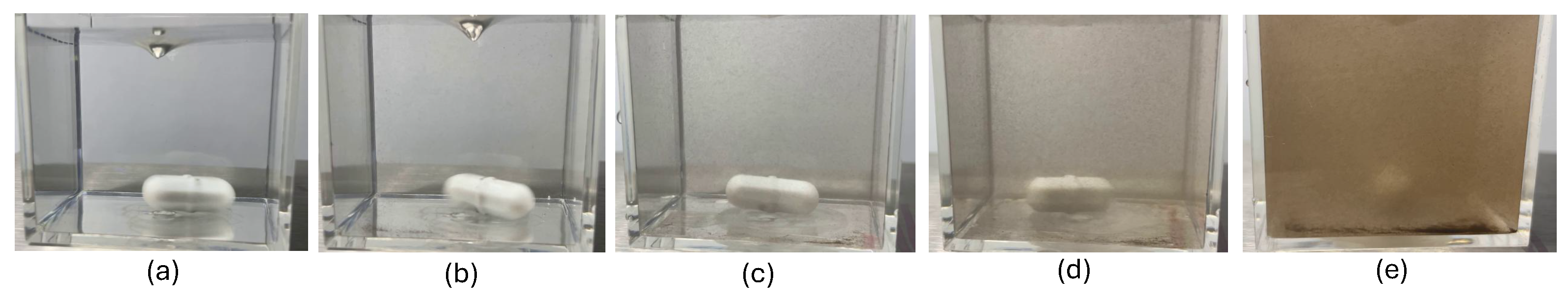
2.1. Sample Generation

Although to date there is no official classification—either in Mexico or internationally—that defines water quality exclusively based on turbidity levels, this study proposes a five-level water quality classification scheme using turbidity as the primary criterion. This proposal is grounded in the current Mexican regulatory framework, which establishes a general five-level classification of water contamination based on different physicochemical parameters, including TSS, as specified in the national water quality indices [33]. To generate the corresponding dataset, 33 water samples with varying turbidity levels were prepared and subsequently classified into five categories: Excellent quality (Class 1), Good quality (Class 2), Acceptable quality (Class 3), Contaminated water (Class 4), and Heavily contaminated (Class 5).

Table 1. Turbidity classes with concentration ranges, standard error percentages, TSS ranges, and number of samples per class.

Class	Turbidity (NTU)	Error (%)	TSS Range (mg/L)	Number of Samples
Excellent quality (Class 1)	0.0–7.0	±10.07	0–25	5
Good quality (Class 2)	10.0–25.0	±5.13	30–80	8
Acceptable quality (Class 3)	30.0–55.0	±3.10	90–150	8
Contaminated (Class 4)	60.0–120.0	±2.39	175–400	8
Highly contaminated (Class 5)	140.0–180.0	±3.95	500–800	4

presents these classes, their corresponding turbidity ranges, the percentage error associated with turbidity measurements (10 repeated measurements), TSS concentration ranges, and the number of samples per class.

The samples were not uniformly distributed across classes due to the natural variation in turbidity levels and operational constraints related to the measurement limits of the turbidimeter. The lowest turbidity class (Class 1) corresponds to very low TSS concentrations, which required precise control during sample preparation, while the highest turbidity class (Class 5) was limited by the maximum measurable threshold of the instrument.

This classification scheme was designed with closed and coherent turbidity intervals to ensure consistency, reproducibility, and to avoid ambiguities arising from overlapping or poorly defined class boundaries. The selected ranges reflect realistic water quality scenarios and provide a scientifically sound framework for training and evaluating the classification models presented in this study.

Moreover, we believe that these turbidity ranges offer a practical and representative overview of contamination degrees in water, which is further supported by the distribution and visual characteristics of the images used in the dataset. Therefore, these classes serve as effective and meaningful categories for water quality classification in this context.

The solids used in sample preparation were primarily sourced from black clays composed of iron and aluminum, which are among the most common solid pollutants in urban environments [34]. To ensure particle size homogeneity, the solids were sieved using a 74-micrometer mesh, allowing controlled particle diameters. The material was then mixed with distilled water to produce samples with varying turbidity levels. Turbidity was measured using a turbidimeter based on the 90° scattering technique, following Mexican regulations. Each measurement was repeated ten times to ensure reproducibility, resulting in a maximum error of ±10.07% NTU. Slight variations among individual measurements are expected due to the movement of suspended particles. This variability is consistent with that reported in similar studies, where standard deviations of up to ±23 NTU have been observed under comparable conditions [21]. It is important to clarify that this value corresponds to the maximum standard deviation obtained experimentally, and not to a regulatory or theoretical threshold. Therefore, the precision obtained in this study is considered acceptable for classification purposes.

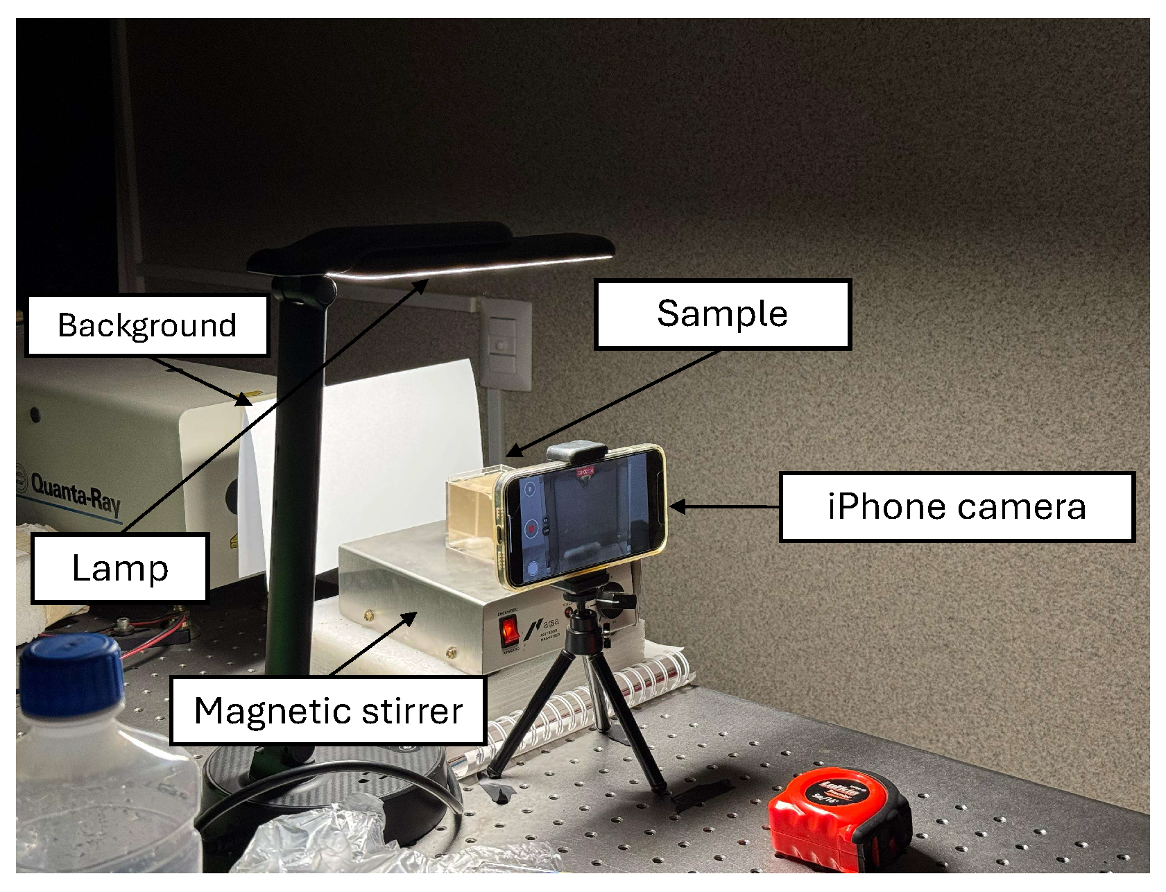
2.2. Image Collection

The image dataset was generated through a controlled experimental setup designed to ensure consistency and high image quality. Water samples with varying turbidity levels were placed in a transparent acrylic cell with dimensions of 5 cm × 5 cm × 5 cm, filled with 120 mL of sample. The cell was positioned on a magnetic stirrer operating at a constant speed of 350 rpm, using a 30 mm hexagonal stirring bar to maintain particle suspension.

Image acquisition was performed using a smartphone camera (Apple iPhone 12) equipped with a 12-megapixel wide-angle sensor (f/1.6 aperture). The camera was positioned 12 cm away from the acrylic cell, with a zoom level of 1.4×, and operated wirelessly to minimize interference. To generate a sufficiently large and diverse dataset for training, videos were recorded for each of the 33 water samples under continuous magnetic stirring, simulating natural particle motion and distribution for one minute. From these videos, frames were extracted at a rate of 6 frames per second, resulting in approximately 360 images per sample. This procedure captures temporal variations and subtle visual differences in turbidity due to suspended solids in motion, providing the CNN with rich information to learn robust features associated with each turbidity class. Images were recorded in full high definition (FHD) at a resolution of $1920\times 1080$ pixels, using the default video mode with automatic exposure and autofocus enabled, to minimize motion blur and ensure consistent image sharpness across all samples.

The images used in this study were captured in RGB format, preserving the full color information of the water samples. This format aligns with the input requirements of the EfficientNet-B0 model employed, which expects three-channel RGB images. The use of RGB images was essential to capture subtle variations in color and turbidity that are critical for accurate classification.

To optimize image quality, the setup included ultra-white lighting positioned 17 cm above the sample, providing uniform top-down illumination. The experiments were conducted in a dark chamber enclosed by blackout curtains to eliminate external light interference. A white background screen was also used to minimize environmental distractions and enhance contrast between the water sample and the background.

Each captured image was cropped to a 500 × 500 pixel matrix to exclude unwanted visual elements such as water vortices, the container base, and other optical distractions. This ensured that the focus remained on a specific, clean region of interest within each image. After this step, all images were carefully reviewed, and several were discarded due to issues such as blurriness, uneven shadows, and the presence of bubbles. In total, approximately 11,800 images were acquired across 33 water samples using a fixed camera and standardized lighting conditions. From this initial set, 362 images were discarded due to visual artifacts such as blur, bubbles, reflections, or the presence of foreign objects. The final dataset used for training and validation included 11,518 curated images. This number of samples proved to be sufficient for robust training, as confirmed by prior work using smaller datasets [32]. Subsequently, the selected images were resized to $244\times 244$ pixels, normalized and standardized per channel (R, G, B) using the mean and standard deviation values from ImageNet, ensuring compatibility with the CNN model used in this study. It is important to note that the images were first cropped to 500 × 500 pixels and subsequently resized to 244 × 244 pixels. This two-step approach was intended to capture a representative portion of the original 1900 × 1080 image, as directly cropping a 244 × 244 pixels region would cover only a small and potentially uninformative fraction of the scene. The entire experimental setup was mounted on a fully leveled table to ensure stability during the image acquisition process. Figure 1 shows the experimental setup and Figure 2 presents a representative image of the samples from each class, contained in $5\times 5\times 5{\mathrm{cm}}^3$ cubic cells under agitation. These images were subsequently processed and cropped to generate the final dataset.

To complement the description of the image acquisition process,

Table 2. Representative RGB images for each turbidity class used in the dataset.

Class 1	Class 2	Class 3	Class 4	Class 5

presents one representative RGB image for each turbidity class, illustrating the appearance of the samples used in model training. Each image corresponds to a sample with a known concentration of TSS and a measured turbidity value, as detailed in Table 1. The visual differences across classes reflect increasing turbidity levels and changes in light scattering patterns caused by suspended particles. These images were captured under standardized conditions to ensure consistency in lighting, positioning, and background. The dataset used for training and validation was entirely composed of images acquired following this setup.

For the classification of turbidity levels in this study, RGB images were acquired under standardized conditions, capturing the visual characteristics of TSS in motion. Rather than relying on manual feature extraction (e.g., gray-level histograms or segmentation of regions of interest), the approach leverages the representational power of CNN. In fact, this is the main advantage of the methodology, where manual feature extraction from images is not necessary. The CNN model was trained to learn complex visual cues—such as variations in color intensity, opacity, and texture—directly from the raw images. These features are implicitly associated with the degree of light scattering caused by suspended particles in water, a well-known optical correlate of turbidity. Thus, the model establishes an indirect but robust mapping between the appearance of the sample and its measured turbidity class.

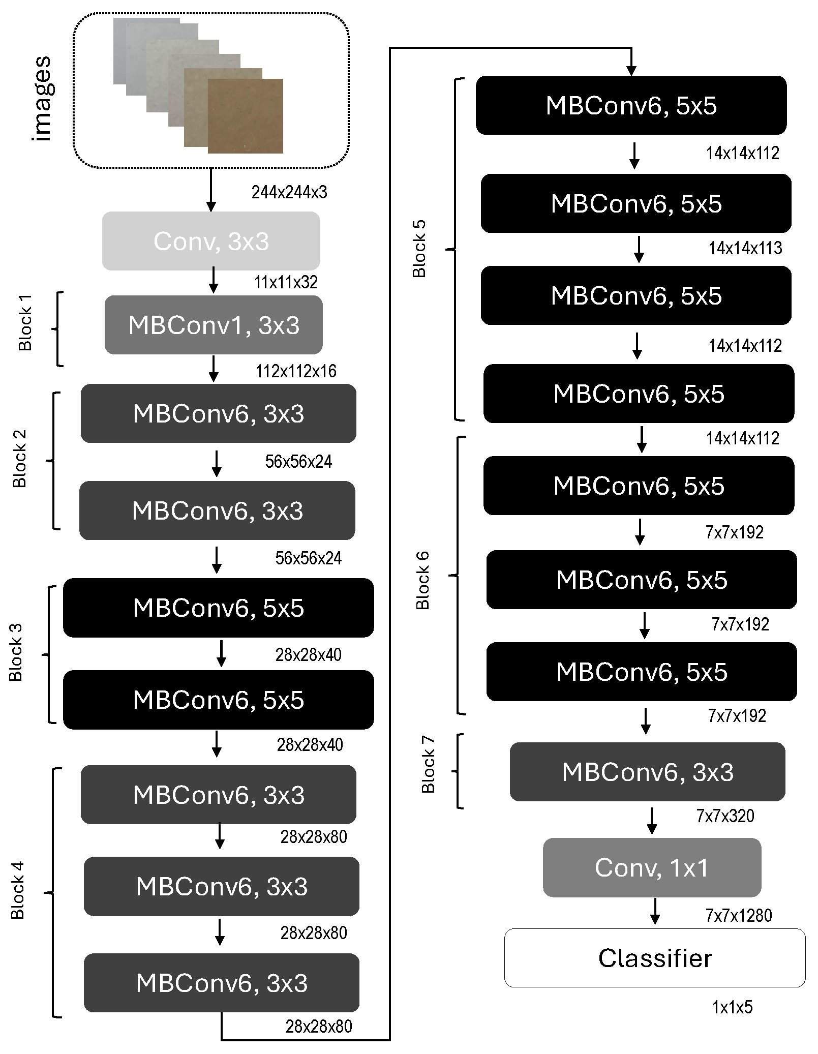
2.3. CNN Model Development

Among the available architectures, EfficientNet-B0, the simplest network in the EfficientNet family, was selected due to its optimized balance between accuracy and computational efficiency. In this study, EfficientNet-B0 was chosen for water classification from images, as it offers a lightweight architecture without sacrificing robust performance in classification tasks. Leveraging a TL approach, the pre-trained EfficientNet-B0 was fine-tuned to adapt to the specific task of water classification from images, significantly reducing training time and improving generalization. This network has the advantage of having been pre-trained on the ImageNet dataset, which contains nearly 150 million diverse images. The original ImageNet classifier was designed to classify 1000 different object categories, which has allowed it to be highly effective in a variety of scientific applications. In the medical field, EfficientNet has been used in brain tumor detection [35], and in the identification of ophthalmic diseases in diabetic patients [36]. Furthermore, it has been used for the classification of gastrointestinal pathologies [37], among other medical applications.

EfficientNet has also demonstrated its effectiveness in other sectors, such as remote sensing, where it has been used to identify water storage tanks [38], and in the forestry sector, for the recognition of oil tea cultivars [39]. Additionally, it has been optimized in lighter versions for tasks such as facial expression recognition [40]. Given its recent evaluation in the classification of TSS in water [41], EfficientNet-B0 was selected for this work due to its stability and superior performance in the comparison of four CNN models, achieving an accuracy of 99.85% in identifying TSS classes. Considering the close relationship between this parameter and turbidity, this model was chosen for its ability to efficiently characterize this variable.

This network was first introduced in [42], making it a relatively recent convolutional architecture. The EfficientNet-B0 model used in this study is detailed in

Table 3. Architecture of the EfficientNet-B0 model used in this study.

Layer	Output Channels	Kernel Size	Stride	Repeat	Additional Information
Conv2d	32	3 × 3	2	1	BatchNorm, SiLU activation
MBConv	16	3 × 3	1	1	SE module, BatchNorm, SiLU
MBConv	24	3 × 3	2	2	SE module, BatchNorm, SiLU
MBConv	40	5 × 5	2	2	SE module, BatchNorm, SiLU
MBConv	80	3 × 3	2	3	SE module, BatchNorm, SiLU
MBConv	112	5 × 5	1	3	SE module, BatchNorm, SiLU
MBConv	192	5 × 5	2	4	SE module, BatchNorm, SiLU
MBConv	320	3 × 3	1	1	SE module, BatchNorm, SiLU
Conv2d	1280	1 × 1	1	1	BatchNorm, SiLU activation
Fully Connected	5	-	-	1	Dropout 0.2, Softmax

and illustrated in Figure 3. It begins with a conventional $3\times 3$ convolution layer, followed by a series of compound mobile inverted bottleneck convolution (MBConv) blocks. These MBConv blocks integrate depthwise separable convolutions—where spatial filtering is first applied to each channel independently, and then combined using $1\times 1$ pointwise convolutions. This technique significantly reduces computational cost compared to traditional approaches. Each MBConv block also incorporates a squeeze-and-excitation (SE) module, inspired by SENet [43], which adaptively recalibrates channel-wise feature responses by explicitly modeling interdependencies between channels. This mechanism enhances the capacity of the network to focus on informative features while suppressing less relevant ones. Furthermore, stochastic depth is applied progressively throughout the network to improve regularization during training. After traversing these stages, the feature maps are processed through a final $1\times 1$ convolution layer, global average pooling, and a fully connected classifier layer. A Softmax activation function is then used to produce the output probabilities across the defined turbidity classes.

In the TL setup, the entire network was retrained without freezing any layers. Initial experiments involving freezing layers did not yield optimal results; complete retraining enabled the model to better adapt to the specific characteristics of the water turbidity dataset. While a formal systematic hyperparameter tuning procedure was not performed, key parameters such as learning rate, batch size, and number of epochs were empirically adjusted over several training runs to achieve a balance between training stability and model performance. This empirical approach led to improved accuracy compared to partial retraining or freezing of layers.

Although CNNs are a well-established approach within the field of ML, their performance depends not only on the dataset but also on several parameters that must be manually defined by the designer. These configuration choices, known as hyperparameters, play a critical role during the training process. Among the most important hyperparameters are epochs, learning rate, optimization algorithm, and batch size [44]. Epochs refer to the number of times the dataset is presented to the network during the training process. Batch size is the number of samples processed before updating the parameters of the model. The optimization algorithm is the method that minimizes the error in each epoch, while simultaneously trying to maximize its accuracy. Another key hyperparameter is the learning rate. If this rate is too low, the model may take many epochs to converge. Conversely, if the rate is too high, it might not converge properly. In this study, all hyperparameters were determined through a trial-and-error approach, gradually adjusting them to achieve satisfactory model performance. The final values used in the model are summarized in

Table 4. Configured hyperparameters employed in the EfficientNet-B0 model.

Hyperparameter	Setting
Algorithm optimizer	Adam
Learning rate	0.0001
Bachsize	50
Epoch	30

.

2.4. CNN Performance Evaluation

To evaluate the performance of the developed CNN, four main metrics were used: accuracy, precision, recall (or sensitivity), and F1-score. These metrics are based on four fundamental values: true positives (TP), which refer to correctly predicted positive outcomes; true negatives (TN), which represent correctly predicted negative outcomes; false negatives (FN), which are images incorrectly classified as negative; and false positives (FP), which are images incorrectly classified as positive. Equations (1)–(4) describe the actual mathematical expressions to obtain these metrics [45].

$$\begin{array}{ccc}\hfill \mathrm{accuracy}& =& \hfill {\displaystyle \frac{\mathrm{TP}+\mathrm{TN}}{\mathrm{TP}+\mathrm{TN}+\mathrm{FP}+\mathrm{FN}}}.\hfill \end{array}$$

(1)

$$\begin{array}{ccc}\hfill \mathrm{precision}& =& \hfill {\displaystyle \frac{\mathrm{TP}}{\mathrm{TP}+\mathrm{FP}}}.\hfill \end{array}$$

(2)

$$\begin{array}{ccc}\hfill \mathrm{recall}& =& \hfill {\displaystyle \frac{\mathrm{TP}}{\mathrm{TP}+\mathrm{FN}}}.\hfill \end{array}$$

(3)

$$\begin{array}{ccc}\hfill \mathrm{F}1-\mathrm{score}& =& \hfill {\displaystyle \frac{2\times \mathrm{recall}\times \mathrm{precision}}{\mathrm{recall}+\mathrm{precision}}}.\hfill \end{array}$$

(4)

For the calculation of the loss during the training process, the cross-entropy loss function was employed. This loss function is commonly used for multi-class classification problems and quantifies the difference between the true class labels and the predicted class probabilities output by the model [46]. Mathematically, the cross-entropy loss L is defined as follows:

$$L=-\sum _{i=1}^N\sum _{c=1}^C{y}_{i,c}log\left({\widehat{y}}_{i,c}\right).$$

(5)

where N is the total number of samples, C is the number of classes, $y_{i,c}$ is a binary indicator that equals 1 if the $i^{\mathrm{th}}$ sample belongs to class c, and 0 otherwise; ${\widehat{y}}_{i,c}$ denotes the predicted probability that the $i^{\mathrm{th}}$ sample belongs to class c.

In addition to these four metrics, the confusion matrix was also derived. This matrix compares the number of images belonging to the actual class with the class predicted by the model. In this matrix, the elements along the diagonal represents correctly classified instances, while the off-diagonal elements correspond to misclassified images. This visualization helps identify which classes the model confuses the most and which images are more difficult to classify, making it a highly illustrative tool.

Finally, the receiver operating characteristic (ROC) curve was also obtained. This curve contrasts the false positive and true positive rates. The ROC curve is accompanied by the area under the curve (AUC), which represents the probability that a randomly selected image is correctly classified. For better interpretation, ROC curves are shown for each class as well as for the overall performance of the model. In this graph, the 45° diagonal line represents a 50% probability. AUC values closer to 1.0 indicate better classification performance.

All the model development and implementation is carried out using Python (version 3.12.4), an open-source, user-friendly, and versatile programming language [47]. The pre-trained EfficientNet-B0 model is obtained from the open-source PyTorch library and implemented within a Jupyter Notebook environment. The development is conducted on a personal computer equipped with an Intel Core i7 processor and CUDA version 12.4. The number of images is divided to the training and validation tests. 75% (8637 images) of the images are used to train and 25% (2881 images) are used to validation.

3. Results

To obtain a robust assessment of the performance of the proposed CNN, it is executed ten times in order to derive more representative metrics, less affected by randomness. In each run, different images are randomly selected for both training and validation. It is worth noting that the images were randomly selected without replacement to ensure unbiased training and testing subsets.

Table 5. Performance metrics with standard deviation and standard error based on 10 runs.

Metric	Validation Value	Standard Deviation	Standard Error
Accuracy	0.9993	0.00137	0.00043
Precision	0.9993	0.00132	0.00041
Recall	0.9993	0.00137	0.00043
F1-score	0.9993	0.00136	0.00042
Loss	0.0020	0.0036	0.00115

presents the average results from the ten runs for accuracy, precision, recall, and F1-score, calculated using Equations (1)–(4) based on the validation data. Additionally, the final loss at epoch 30 is also reported.

For the evaluation of the classification system, the confusion matrix corresponding to one of the runs of the model is presented in Figure 4. This matrix visually summarizes the results obtained from the 2881 images used during the validation phase. We can see that the model achieves nearly 100% accuracy across all classes. A minimal degree of misclassification of 0.005 was observed only for the Excellent quality (Class 1) category, where two images were incorrectly predicted as belonging to the Good quality (Class 2) class. In contrast, all images from Class 2 were correctly classified, suggesting that the model had no difficulty identifying this class. The confusion is likely due to the visual similarity between the two adjacent categories.

Continuing with the evaluation, the multi-class ROC curve is presented in Figure 5, along with the AUC for each of the proposed turbidity classes. The curve indicates that all classes exhibit a high level of accurate classification. In general, there is a strong tendency toward an optimal relationship between the true positive rate (TPR) and the false positive rate (FPR), with most classes approaching a TPR close to 1.0 and an FPR near zero—suggesting a nearly perfect classification performance.

In order to rule out potential overfitting during the training and validation processes, continuous monitoring of both accuracy and loss functions was conducted throughout the epochs. Figure 6 presents these learning curves: panel (a) shows the overall accuracy versus epochs for both the training and validation datasets, while panel (b) displays the corresponding loss values. The x-axis represents the number of epochs, and the y-axis shows the respective accuracy or loss metrics. It can be observed that the model and optimization algorithm perform effectively, with accuracy improving and loss progressively decreasing as training advances. The accuracy starts at a relatively high value of approximately 92% and improves rapidly within the first five epochs, quickly reaching about 99%. Although the initial loss value is approximately 0.30, it steadily declines, and no significant fluctuations appear in the loss curves, indicating stability throughout the learning process.

4. Discussion

As demonstrated in Table 5, the EfficientNet-B0 model achieved outstanding performance in turbidity image classification, consistently exceeding metrics of 0.99 for accuracy, precision, recall, and F1-score across multiple independent runs. These results were obtained using different training/validation splittings of the datasets. Furthermore, the standard deviation and error standard observed are minimal—0.0013 and 0.0004, respectively—indicating that the performance of the model remains remarkably stable, despite multiple executions, demonstrating a strong generalization capability of the model.

Regarding the classification performance of the network, the confusion matrix in Figure 4 reveals that it is possible to identify that Class 1 and Class 2—corresponding to Excellent quality and Good quality water, respectively—appear to be the most difficult to classify. These two classes exhibit the lowest turbidity levels, with Excellent quality defined by turbidity values ranging from 0.0 to 7.0 NTU, and Good quality ranging approximately from 10–25 NTU. These represent samples with minimal turbidity measurements. However, the degree of misclassification between these two classes is very low. Only 0.005 of the Class 1 samples, namely one image, is incorrectly classified as belonging to Class 2. The overall low turbidity values in both classes likely contribute to occasional confusion, especially for samples with turbidity values near the decision boundary between the two classes. In contrast, the model demonstrates a clear ability to distinguish among the remaining classes, where no significant classification difficulties are observed.

The ROC curve in Figure 5 and the corresponding AUC values obtained provide a general overview of the ability of the model to correctly classify each class. The AUC values indicate an almost perfect prediction probability of 1.00 for each class as well as overall, suggesting the highest accurate classification performance across all categories.

Overall, the results demonstrate the robustness and reliability of the proposed model in classifying turbidity levels based on visual features. However, the minor misclassification observed between Class 1 and Class 2 highlights a subtle yet important challenge. These two categories represent the lowest turbidity levels, with a narrow separation threshold corresponding to approximately 25 mg/L (i.e., 0.025 g/L) of TSS. Given this minimal concentration difference, the optical appearance of some samples near this boundary is highly similar. As shown in Table 2, the initial images of Class 2 closely resemble those of Class 1, making the visual distinction between them particularly difficult—even for human observers. This explains why the model occasionally confuses these two adjacent categories. Such behavior suggests that the classification of very low turbidity levels may require either higher-resolution imaging, additional spectral information, or a refined labeling protocol to minimize ambiguity at critical thresholds.

Regarding the learning curves shown in Figure 6, the model exhibits an initially high accuracy (Figure 6a) and relatively low loss (Figure 6b) at the start of training. This behavior is consistent with the expected advantage of TL, where the model leverages prior knowledge from large pre-trained datasets, thereby improving convergence speed and initial performance.

4.1. Representative Classification Examples

Additionally, to illustrate the performance of the proposed CNN model, a subset of 5000 images was randomly selected from both the training and validation datasets. This subset provides a representative sample of the overall data distribution and enables a detailed examination of model behavior across the dataset employed.

Figure 7 presents representative images corresponding to the four primary classification outcomes: TP, TN, FP, and FN. Each example shows the input image along with its actual and predicted class labels, allowing visual assessment of the classification accuracy of the model.

These examples serve to highlight the strengths and limitations of the model. The CNN achieves high accuracy in cases where inter-class differences in turbidity levels manifest as distinct colorimetric and textural features. However, classification errors primarily occur between adjacent turbidity classes, which exhibit more subtle visual distinctions. This behavior is consistent with the performance trends previously shown in Section 3, where reduced precision and recall were observed in the most visually similar classes (e.g., Class 1 vs. Class 2).

4.2. Comparison with Similar Studies

Table 6. Proposed model vs. other works.

Method	Accuracy	Year	Reference
EfficientNet-B0 CNN model with TL approach	99.93%	2025	This work
Designed shallow CNN model with data augmentation	94.34–98.42%	2024	[48]
Designed CNN model with sintetic samples of formazine and kaolin clays	90.9–98.7%	2024	[49]
Customized 4 CNN models: 8 layers, 8 layers with dropout, 10 layers, and 10 layers with dropout, trained with synthetic samples of turbidity caused by calcium carbonate (CaCO3)	84.0–88.0%	2025	[50]
Shallow desainged CNN with laboratory and real samples	97 (laboratory samples)–85% (real samples)	2024	[51]
Designed a 5 layers CNN model with 3 fully-conected layers	87.5–97.5%	2023	[26]

shows the results of some recent studies focused on the classification of different turbidity levels that have also addressed turbidity classification using different CNN architectures,. In each of these works, different materials to simulate turbidity—such as formazine, kaolin clays, or calcium carbonate—were used, including real samples for validation purposes.

From Table 6, we can observe that despite methodological differences, our work achieves an almost perfect accuracy. This outcome is expected, given that our CNN model is a deep learning architecture characterized by a large number of layers, in contrast to the shallower CNNs implemented in other studies. An additional advantage of our approach is the integration of TL, which takes advantage of pre-trained networks. This allows the model to already possess the ability to extract relevant features from images, making it a highly efficient technique that enhances the performance and evaluation metrics of the CNN. This advantage is further supported by recent studies such as [20], where a pre-trained YOLOv8-based CNN combined with TL achieved 100% accuracy, and [21], in which a pre-trained AlexNet model was successfully used to predict turbidity levels and concentrations. While previous studies have reported slightly higher accuracy, this may be partly attributed to differences in model design and dataset size. The referenced YOLOv8-based system uses a real-time object detection framework, which is structurally different from the image classification approach in our study. Additionally, the AlexNet-based model, although shallower than EfficientNet-B0, was trained on a dataset of approximately 88,000 images, compared to the 11,518 images used here. This difference in training data volume likely contributes to the small performance gap.

Furthermore, recent studies have demonstrated the effectiveness of traditional ML algorithms in predicting water turbidity across diverse environmental settings. For example, in [52], the authors applied a long short-term memory recurrent neural network (LSTM-RNN) to marine environments and reported a high prediction accuracy of 88.45%, outperforming conventional neural networks and support vector regression. For inland water bodies, in [53], a decision tree regression was employed on remote sensing data to predict lake turbidity, achieving a coefficient of determination (R²) of 0.776. Additionally, in [28], a Bayesian neural network (BNN) modeling framework was developed to predict water turbidity with efficiencies greater than 0.87 during training and 0.73 during validation. Although these studies demonstrate strong performance, our approach offers the advantage of relying solely on analyzed images without the need for additional variables, making it simpler and practical. Moreover, our model achieves higher accuracy, with a reported accuracy of approximately 99%, indicating superior predictive capability.

In addition to the literature review, we developed and evaluated two alternative machine learning classification systems to benchmark the performance of the CNN model. Specifically, we implemented a random forest classifier and a multi-layer perceptron (MLP) neural network. For both approaches, 75% of the original image dataset was used for training and 25% for validation. To represent the images numerically, we extracted texture-based features such as contrast, correlation, and energy from the gray-scale.

For the random forest model, we used an ensemble of 100 decision trees. The model was trained using a stratified train–test split with a fixed random seed to ensure reproducibility and proper class distribution across training and validation sets. No normalization or feature scaling was applied, as tree-based models are invariant to the scale of the input features. The MLP architecture consisted of two hidden layers with 128 and 64 neurons, respectively, using the ReLU activation function. The MLP model was trained for 30 epochs using the Adam optimizer with a learning rate of 0.0001, consistent with the training configuration of the CNN model. This setting provided stable convergence and facilitated a fair comparison between both approaches.

Table 7. Comparison of performance metrics for CNN, Random Forest, and MLP classifiers.

Model	Accuracy	Precision	Recall	F1-Score
CNN (EfficientNet-B0 + TL)	99.85%	99.85%	99.85%	99.86%
Random Forest	99.62%	99.58%	99.56%	99.57%
MLP	94.58%	95.08%	93%	94%

summarizes the accuracy, precision, recall, and F1-score obtained for each method on the validation dataset.

The CNN model achieved the highest overall accuracy among the evaluated models, reaching 99.85%. Both the random forest and MLP classifiers demonstrated competitive performance, as summarized in Table 7. The random forest classifier achieved near-perfect metrics, with an overall accuracy of 99.62%, precision of 99.58%, recall of 99.56%, and F1-score of 99.57%. This excellent performance is notable considering that this machine learning method relied solely on texture features extracted from the images. However, the relatively small feature set might limit the ability of the model to generalize to more complex or diverse datasets.

While the random forest classifier yielded competitive performance on the original training and validation sets, its generalization capacity proved to be the most limited among the evaluated models when exposed to unseen data. Specifically, as shown in Appendix C, the model collapsed under minimal distributional shifts introduced by a new red clay-based dataset—misclassifying nearly all samples as Class 5. This outcome highlights a critical limitation: unlike CNN architectures, random forest does not leverage spatial hierarchies or deep feature representations, making it particularly vulnerable when the extracted descriptors (e.g., color and texture) deviate from the training distribution. In contrast, the CNN model benefits from its deep architecture and TL approach, allowing it to automatically learn complex hierarchical features directly from raw image data. This capability eliminates the need for manual feature extraction, making the CNN approach not only more scalable and adaptable but also more efficient and less dependent on domain-specific knowledge.

The MLP classifier achieved an overall accuracy of 95%, with precision, recall, and F1-scores slightly lower at 95%, 93%, and 94%, respectively. Notably, class-specific performance varied, with reduced recall observed in some classes, which may indicate challenges in distinguishing certain turbidity levels using the selected handcrafted features. We believe that improved performance could be achieved by employing a deeper neural network architecture or increasing the number of training epochs.

It is important to note that the high performance of the models is supported by the rigorous image acquisition protocol and strict quality control of the training dataset. Consistent lighting conditions, proper focus, and careful image selection minimized noise and variability, enabling the model to learn effectively from high-quality data. This attention to image quality plays a key role in achieving reliable classification results. Furthermore, the use of the EfficientNet-B0 architecture, known for its balance between depth and efficiency, allows for effective feature extraction from RGB images while maintaining a lightweight structure. Additionally, the integration of TL enables the model to leverage pre-trained knowledge, improving generalization even with a moderate-size dataset. Image acquisition was performed under standardized conditions—including controlled lighting, background, and positioning—which reduced visual variability and enhanced the consistency of the training data. Moreover, the turbidity classification scheme employed is based on well-defined thresholds with corresponding TSS concentrations, reducing ambiguity in class labeling. Altogether, these aspects contribute to the strong classification results observed in this study.

4.3. Model Limitations

Although the EfficientNet-B0 model achieved nearly perfect performance on laboratory-prepared samples, these consisted of clay suspensions in distilled water under consistent lighting and imaging conditions. This controlled setup enabled reliable baseline testing but does not yet encompass the full range of variability found in natural environments, where turbidity may result from complex mixtures of suspended solids, organic matter, and microorganisms. As such, the current performance of the model reflects its ability to classify turbidity within a well-defined and homogeneous scenario. Further work is needed to extend the dataset with more diverse samples and acquisition settings, which will support the development of a more robust and generalizable model.

Nevertheless, despite the fact that the model is trained exclusively on laboratory samples, this work represents a foundational step in the development of a vision-based classification system for water quality assessment. It provides a stable and reproducible framework for future extensions to field conditions (see Appendix A for details on the validation procedure with additional samples). Moreover, as demonstrated in [51], models trained in controlled environments can be effectively adapted to real-world applications through appropriate calibration, as our group is planning for the near future.

Regarding the turbidity class thresholds defined in this study, which include gaps between classes (e.g., between 7 and 10 NTU and 25–30 NTU), we stress that these gaps are not imposed arbitrarily, but arise naturally from the experimental procedure and sample preparation, since the turbidity values are classified according to corresponding TSS concentrations. Variations in TSS directly influence turbidity readings, which explains the observed non-continuous ranges in turbidity classes. This deserves special attention, for instance, when samples with near-threshold turbidity values (7.0–10 NTU) are considered, because although small, the minimal misclassification observed between Class 1 and Class 2 might demand a different approach to be resolved.

Another limitation is that the maximum turbidity level tested was 180 NTU, which may not encompass the highest values found in natural waters. Nonetheless, the proposed model offers a practical assessment of water quality, and extreme turbidity levels are usually visually apparent without relying solely on instrumental measurements or models. Additionally, this study used a single imaging device, the iPhone 12, which applies internal image enhancement that may influence the visual features extracted by the model. Future research would explore the performance of the proposed method using a wider range of cameras, including those with lower and higher dynamic ranges, to evaluate robustness and generalizability across different imaging conditions.

To evaluate the impact of normalization on model performance, we conducted a test using a subset of 1000 images per class without applying prior normalization. The results indicate that the absence of normalization causes a collapse in classification quality, with a significant increase in misclassifications and class confusions, resulting in a chaotic model behavior. This is clearly illustrated in the confusion matrix shown in Figure 8, where most predictions are incorrectly assigned—even among classes that are distinct in feature space. This experiment highlights the critical need for normalization to ensure proper model functioning. Although normalization might restrict the ability of the model to generalize to more heterogeneous data—given that the model was specifically designed and trained to receive normalized images—it confirms that this preprocessing step is essential to maintain acceptable classification performance under the current dataset conditions.

Furthermore, to evaluate the susceptibility of the proposed CNN model to variations in image acquisition, an additional test was conducted using randomly cropped image regions as a surrogate for suboptimal framing conditions. Given that the original dataset was collected under controlled settings with consistent positioning, lighting, and framing, this analysis aims to assess the model robustness when faced with spatial perturbations commonly encountered in real-world scenarios.

Using the RandomCrop transformation from the torchvision.transforms library, a new dataset comprising 5000 cropped samples was generated, evenly distributed across the five turbidity classes (1000 images per class). These crops targeted the region of interest in each image, introducing variability in the captured content and simulating deviations in sample positioning or camera alignment. These results are summarized in

Table 8. Classification metrics for the CNN model evaluated with randomly cropped images.

Class	Precision	Recall	F1-Score	Images Evaluated
Class 1	0.9882	0.9190	0.9523	1000
Class 2	0.8821	0.7560	0.8142	1000
Class 3	0.8003	0.9540	0.8704	1000
Class 4	0.9725	0.9900	0.9812	1000
Class 5	0.9880	0.9910	0.9895	1000
Accuracy	0.9220 (5000 total samples)

, while the confusion matrix shown in Figure 9 highlights class-wise misclassification patterns. The model attained an overall accuracy of 92.20%, with high precision and recall for most classes. Notably, some performance degradation was observed, particularly for Class 2, where recall dropped to 75.60%. This outcome suggests that while the model exhibits a commendable degree of generalization to spatially altered inputs, it remains partially sensitive to changes in framing and positioning. This limitation is inherent to CNN-based architectures trained on homogeneous and consistently structured datasets, which can lead to overfitting to spatial regularities. Therefore, although the model maintains strong performance under moderate deviations, its classification accuracy is not entirely invariant to acquisition conditions. Future work should explore additional training strategies—such as spatial augmentation or domain randomization—to further enhance robustness in deployment scenarios.

Despite its limitations, the model achieved very high performance, demonstrating the potential of this approach. This work establishes a benchmark for a vision-based system for water quality classification, while working with real water samples presents significant challenges, this study serves as a precedent to develop and refine methodologies that can be adapted to diverse water quality scenarios. By combining TL with a novel, lightweight architecture (EfficientNet-B0), an optimized image acquisition protocol, and a multi-class turbidity classification approach, the study offers new insights into image-based water quality assessment and lays the groundwork for future field-scale implementations.

Nevertheless, while the method shows potential as a low-cost tool for turbidity classification, we acknowledge that this benefit cannot be fully confirmed without further validation using real-world water samples.

5. Conclusions

This study evaluated the performance of a deep learning approach for turbidity classification based on images using the EfficientNet-B0 architecture. The main conclusions are as follows:

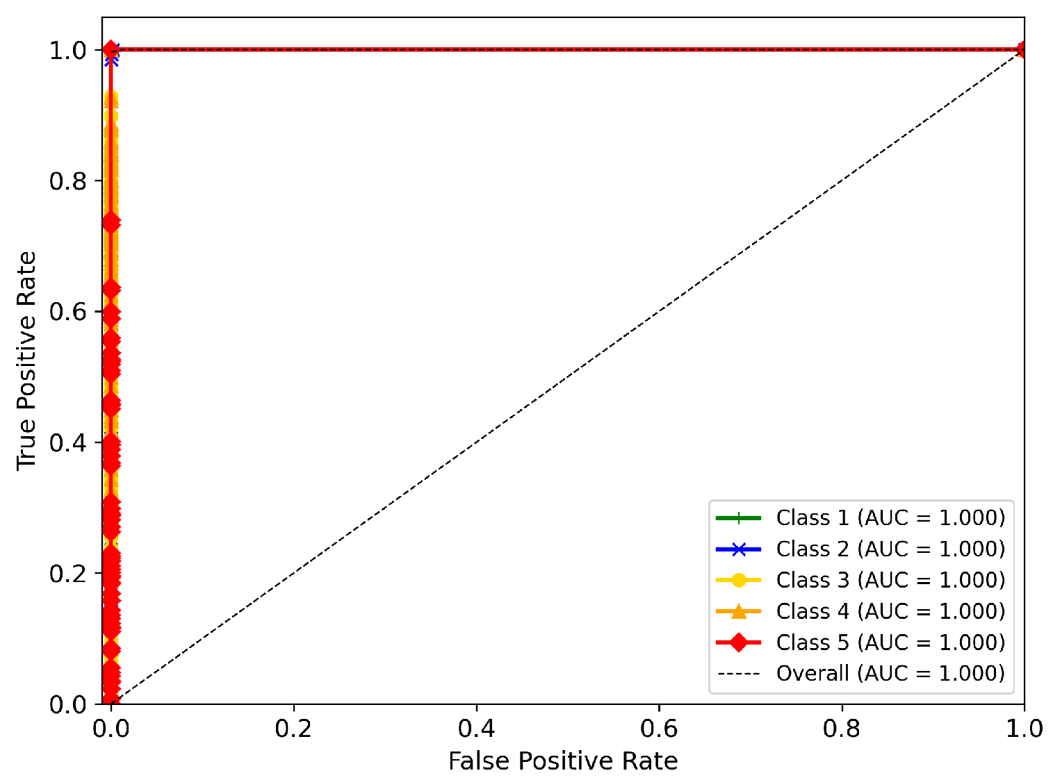
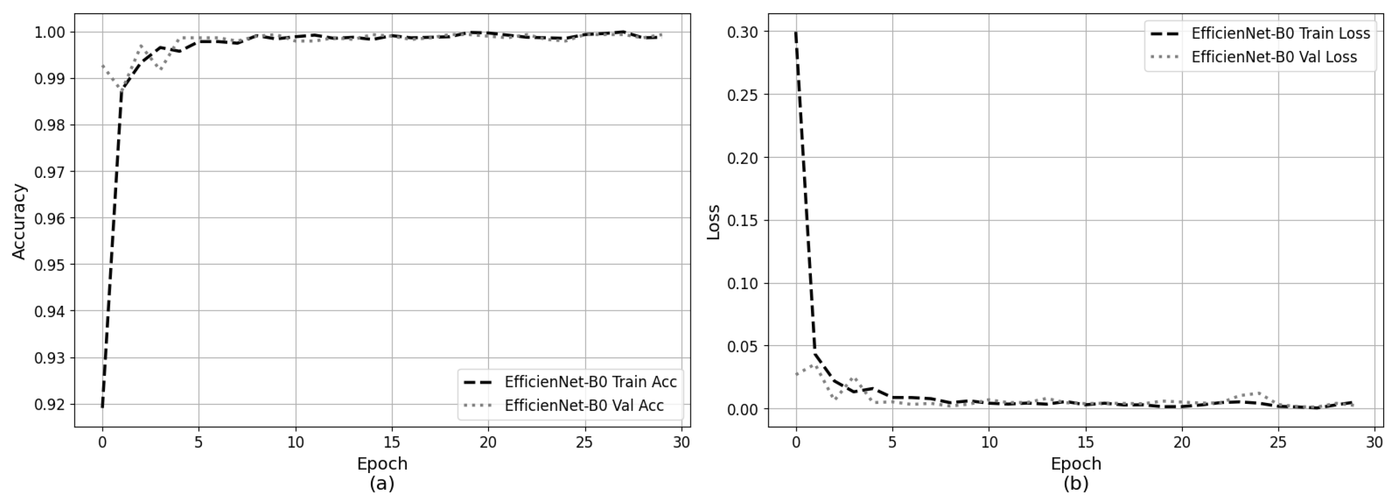
• The proposed CNN model achieved outstanding accuracy (99.93%) in classifying five turbidity levels, showing high precision, recall, and F1-score across multiple runs with low variability.
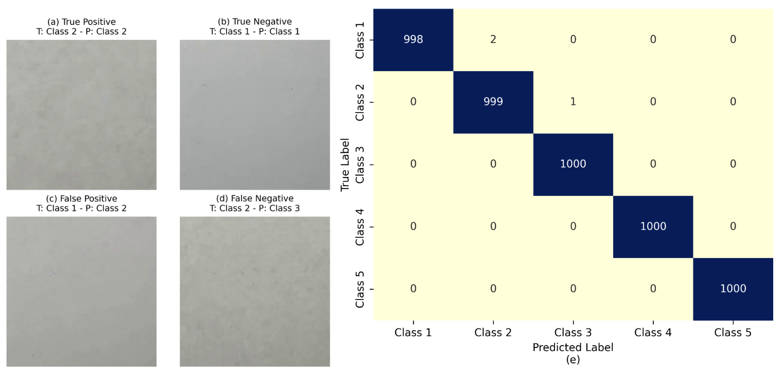
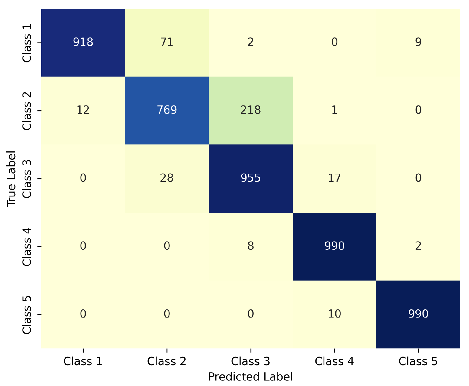
• Most classification errors occurred between Class 1 and Class 2, which correspond to low turbidity levels with subtle visual differences. This suggests the need for enhanced resolution or additional spectral information for borderline cases.
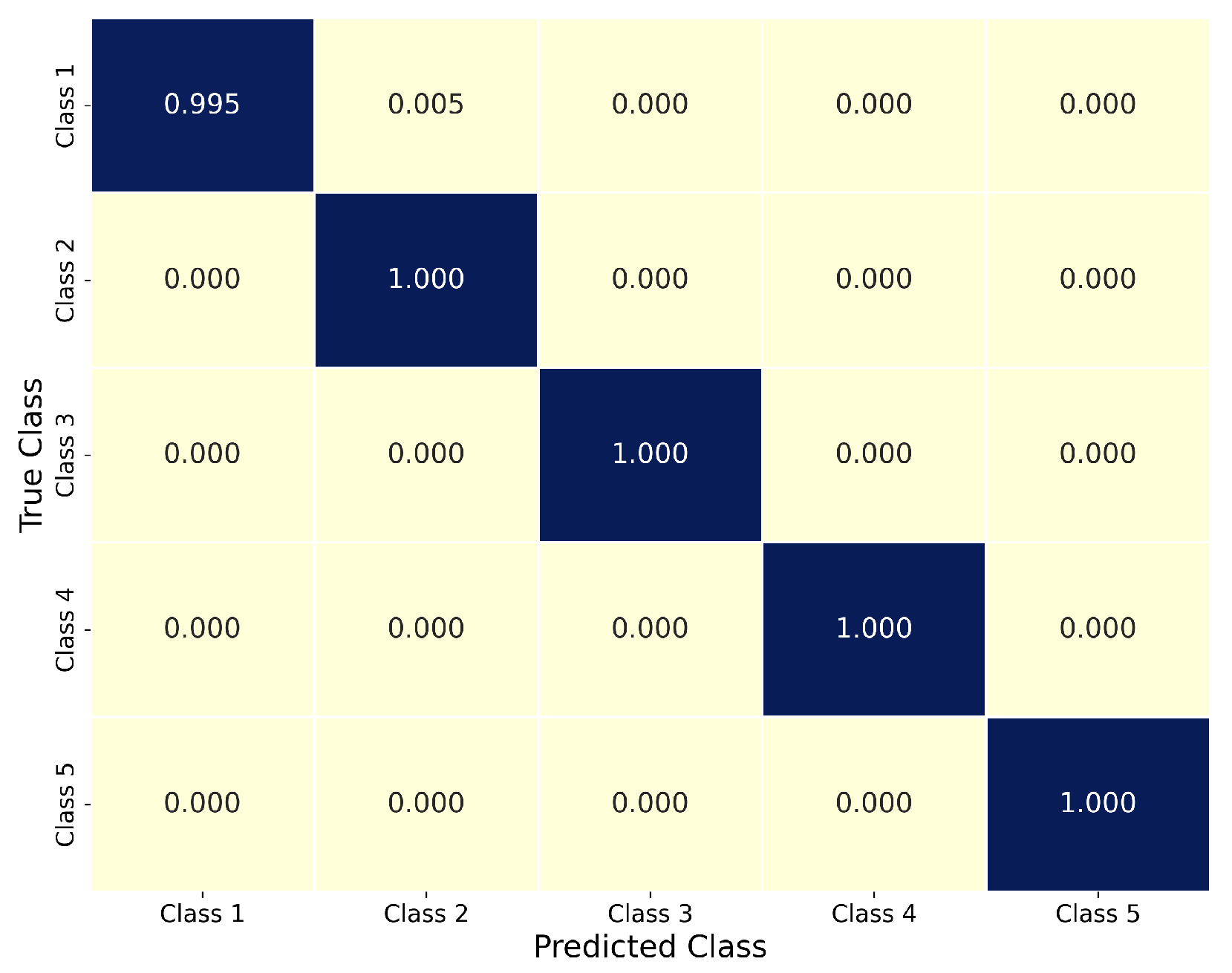
• Representative classification examples and confusion matrices confirm the robustness of the model and highlight its limitations, particularly for adjacent classes with overlapping features.
• Compared to previous studies, the proposed model outperformed other CNN-based approaches, benefiting from the use of TL and a standardized image acquisition protocol.
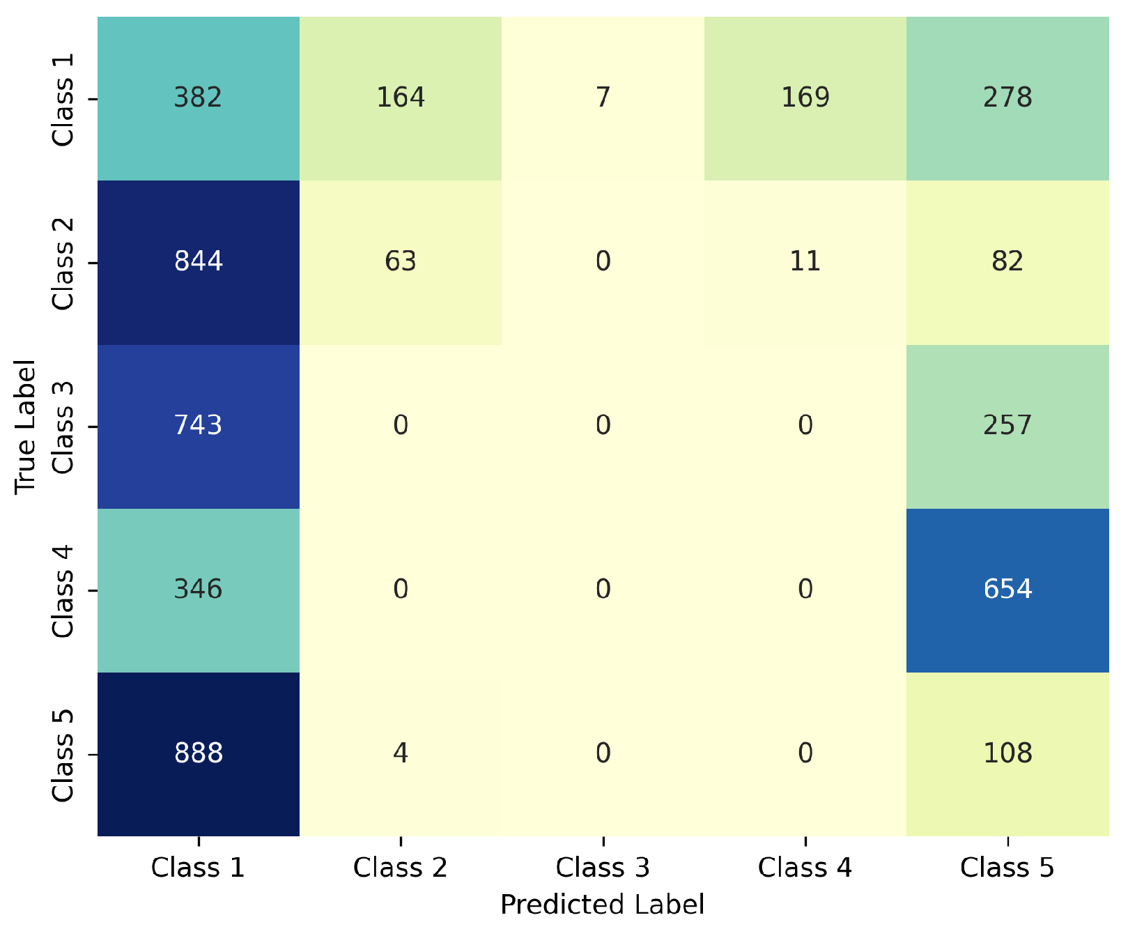
• Although trained exclusively with laboratory-prepared samples, the model establishes a reproducible framework that can be extended to real-world water conditions with appropriate validation (see Appendix A).
• Future work will include expanding the dataset with real water samples, increasing the number of samples in low-turbidity classes, and incorporating real water conditions to improve model generalizability and support claims of broader applicability.
• Additionally, we plan to evaluate the effect of different camera types and image resolutions on model performance, in order to assess their influence on classification accuracy and error propagation.

References

1. National Water Commission (CONAGUA). Laboratories of the National Water Commission. 2025. Available online: https://laboratorios.conagua.gob.mx:8446/LABORATORIOS/Pages/Laboratorios.aspx (accessed on 8 April 2025).
2. Miljojkovic, D.; Trepsic, I.; Milovancevic, M. Assessment of physical and chemical indicators on water turbidity. Phys. A Stat. Mech. Its Appl. 2019, 527, 121171. [Google Scholar] [CrossRef]
3. West, A.O.; Scott, J.T. Black disk visibility, turbidity, and total suspended solids in rivers: A comparative evaluation. Limnol. Oceanogr. Methods 2016, 14, 658–667. [Google Scholar] [CrossRef]
4. Farrell, C.; Hassard, F.; Jefferson, B.; Leziart, T.; Nocker, A.; Jarvis, P. Turbidity composition and the relationship with microbial attachment and UV inactivation efficacy. Sci. Total Environ. 2018, 624, 638–647. [Google Scholar] [CrossRef] [PubMed]
5. Dunlop, J.; McGregor, G.; Horrigan, N. Potential impacts of salinity and turbidity in riverine ecosystems. In National Action Plan for Salinity and Water Quality, State of Queensland; Department of Natural Resources and Mines: Brisbane, QLD, Australia, 2005. [Google Scholar]
6. Lloyd, D.S. Turbidity as a water quality standard for salmonid habitats in Alaska. N. Am. J. Fish. Manag. 1987, 7, 34–45. [Google Scholar] [CrossRef]
7. Huey, G.M.; Meyer, M.L. Turbidity as an indicator of water quality in diverse watersheds of the upper Pecos River basin. Water 2010, 2, 273–284. [Google Scholar] [CrossRef]
8. Packman, J.J.; Comings, K.J.; Booth, D.B. Using turbidity to determine total suspended solids in urbanizing streams in the Puget Lowlands. In Confronting Uncertainty: Managing Change in Water Resources and the Environment, Canadian Water Resources Association Annual Meeting, Vancouver, BC, Canada, 27–29 October 1999; Canadian Water Resources Association: Vancouver, BC, Canada, 1999; pp. 158–165. Available online: http://hdl.handle.net/1773/16333 (accessed on 30 April 2025).
9. Gippel, C.J. Potential of turbidity monitoring for measuring the transport of suspended solids in streams. Hydrol. Process. 1995, 9, 83–97. [Google Scholar] [CrossRef]
10. Grayson, R.B.; Finlayson, B.L.; Gippel, C.J.; Hart, B.T. The potential of field turbidity measurements for the computation of total phosphorus and suspended solids loads. J. Environ. Manag. 1996, 47, 257–267. [Google Scholar] [CrossRef]
11. Omar, A.F.B.; MatJafri, M.Z.B. Turbidimeter design and analysis: A review on optical fiber sensors for the measurement of water turbidity. Sensors 2009, 9, 8311–8335. [Google Scholar] [CrossRef] [PubMed]
12. Secretaría de Economía. NMX-AA-038-SCFI-2001: Water Analysis—Determination of Turbidity in Natural, Wastewater, and Treated Wastewater—Test Method; Cancels NMX-AA-038-1981. CDU: 543.31/.38; Secretaría de Economía: Mexico City, Mexico, 2001.
13. Fu, G.; Jin, Y.; Sun, S.; Yuan, Z.; Butler, D. The role of deep learning in urban water management: A critical review. Water Res. 2022, 223, 118973. [Google Scholar] [CrossRef] [PubMed]
14. Benisi Ghadim, H.; Salarijazi, M.; Ahmadianfar, I.; Heydari, M.; Zhang, T. Developing a sediment rating curve model using the curve slope. Pol. J. Environ. Stud. 2020, 29, 1151–1159. [Google Scholar] [CrossRef] [PubMed]
15. Lewis, D.J.; Tate, K.W.; Dahlgren, R.A.; Newell, J. Turbidity and total suspended solid concentration dynamics in streamflow from California oak woodland watersheds. In Proceedings of the Fifth Symposium on Oak Woodlands: Oaks in California’s Challenging Landscape, San Diego, CA, USA, 22–25 October 2001; Gen. Tech. Rep. PSW-GTR-184. Standiford, R.B., Ed.; Pacific Southwest Research Station, Forest Service, U.S. Department of Agriculture: Albany, CA, USA, 2002; pp. 107–118. [Google Scholar]
16. Nikoonahad, A.; Ebrahimi, A.A.; Nikoonahad, E.; Ghelmani, S.V.; Mohammadi, A. Evaluation the correlation between turbidity and total suspended solids with other chemical parameters in Yazd wastewater treatment effluent plant. J. Environ. Health Sustain. Dev. 2016, 1, 78–86. [Google Scholar]
17. Anderson, P.; Davie, R.D. Use of Transparency Tubes for Rapid Assessment of Total Suspended Solids and Turbidity in Streams. Lake Reserv. Manag. 2004, 20, 110–120. [Google Scholar] [CrossRef]
18. Villa, A.; Fölster, J.; Kyllmar, K. Determining suspended solids and total phosphorus from turbidity: Comparison of high-frequency sampling with conventional monitoring methods. Environ. Monit. Assess. 2019, 191, 605. [Google Scholar] [CrossRef] [PubMed]
19. Hannouche, A.; Chebbo, G.; Joannis, C.; Ruban, G.; Tassin, B. Relationship between turbidity and total suspended solids concentration within a combined sewer system. Water Sci. Technol. 2011, 64, 2445–2452. [Google Scholar] [CrossRef] [PubMed]
20. Rudy, I.M.; Wilson, M.J. Turbidivision: A computer vision application for estimating turbidity from underwater images. PeerJ 2024, 12, e18254. [Google Scholar] [CrossRef] [PubMed]
21. Lopez-Betancur, D.; Moreno, I.; Guerrero-Mendez, C.; Saucedo-Anaya, T.; González, E.; Bautista-Capetillo, C.; González-Trinidad, J. Convolutional neural network for measurement of suspended solids and turbidity. Appl. Sci. 2022, 12, 6079. [Google Scholar] [CrossRef]
22. Mullins, D.; Coburn, D.; Hannon, L.; Jones, E.; Clifford, E.; Glavin, M. A novel image processing-based system for turbidity measurement in domestic and industrial wastewater. Water Sci. Technol. 2018, 77, 1469–1482. [Google Scholar] [CrossRef] [PubMed]
23. Guapacho, J.J.; Guativa, J.A.V.; Baquero, J.E.M. Analysis of artificial vision techniques for implementation of virtual instrumentation system to measure water turbidity. J. Eng. Sci. Technol. Rev. 2021, 14, 161–168. [Google Scholar] [CrossRef]
24. Parra, L.; Ahmad, A.; Sendra, S.; Lloret, J.; Lorenz, P. Combination of machine learning and RGB sensors to quantify and classify water turbidity. Chemosensors 2024, 12, 34. [Google Scholar] [CrossRef]
25. Cao, P.; Zhao, W.; Liu, S.; Shi, L.; Gao, H. Using a digital camera combined with fitting algorithm and T-S fuzzy neural network to determine the turbidity in water. IEEE Access 2019, 7, 83589–83599. [Google Scholar] [CrossRef]
26. Feizi, H.; Sattari, M.T.; Mosaferi, M.; Apaydin, H.A.L.İ.T. An image-based deep learning model for water turbidity estimation in laboratory conditions. Int. J. Environ. Sci. Technol. 2023, 20, 149–160. [Google Scholar] [CrossRef]
27. Magrì, S.; Ottaviani, E.; Prampolini, E.; Besio, G.; Fabiano, B.; Federici, B. Application of machine learning techniques to derive sea water turbidity from Sentinel-2 imagery. Remote Sens. Appl. Soc. Environ. 2023, 30, 100951. [Google Scholar] [CrossRef]
28. Huang, J.; Qian, R.; Gao, J.; Bing, H.; Huang, Q.; Qi, L.; Song, S.; Huang, J. A novel framework to predict water turbidity using Bayesian modeling. Water Res. 2021, 202, 117406. [Google Scholar] [CrossRef] [PubMed]
29. Zhang, Y.; Yao, X.; Wu, Q.; Huang, Y.; Zhou, Z.; Yang, J.; Liu, X. Turbidity prediction of lake-type raw water using random forest model based on meteorological data: A case study of Tai lake, China. J. Environ. Manag. 2021, 290, 112657. [Google Scholar] [CrossRef] [PubMed]
30. Song, C.; Zhang, H. Study on turbidity prediction method of reservoirs based on long short term memory neural network. Ecol. Model. 2020, 432, 109210. [Google Scholar] [CrossRef]
31. Risfendra, R.; Ananda, G.F.; Setyawan, H. Deep learning-based waste classification with transfer learning using EfficientNet-B0 model. J. Resti (Rekayasa Sist. Dan Teknol. Inf.) 2024, 8, 535–541. [Google Scholar] [CrossRef]
32. Luviano Soto, I.; Sánchez, Y.C.; Raya, A. Water quality polluted by total suspended solids classified within an artificial neural network approach. Water Qual. Res. J. 2025, 60, 214–228. [Google Scholar] [CrossRef]
33. SEMARNAT (Secretariat of Environment and Natural Resources). Water Quality Indicators. Government of Mexico. 2020. Available online: https://apps1.semarnat.gob.mx:8443/dgeia/compendio_2020/dgeiawf.semarnat.gob.mx_8080/approot/dgeia_mce/html/RECUADROS_INT_GLOS/D3_AGUA/D3_AGUA04/D3_R_AGUA05_01.htm (accessed on 25 March 2025).
34. Perry, C.; Taylor, K. Environmental Sedimentology; John Wiley & Sons, Blackwell Publishing: Malden, MA, USA, 2009. [Google Scholar]
35. Nayak, D.R.; Padhy, N.; Mallick, P.K.; Zymbler, M.; Kumar, S. Brain tumor classification using dense efficient-net. Axioms 2022, 11, 34. [Google Scholar] [CrossRef]
36. Shahriar Maswood, M.M.; Hussain, T.; Khan, M.B.; Islam, M.T.; Alharbi, A.G. CNN based detection of the severity of diabetic retinopathy from the fundus photography using EfficientNet-B5. In Proceedings of the 2020 11th IEEE Annual Information Technology, Electronics and Mobile Communication Conference (IEMCON), Virtual, 4–7 November 2020; IEEE: Piscataway, NJ, USA, 2020. [Google Scholar]
37. UÇan, M.; Kaya, B.; Kaya, M. Multi-class gastrointestinal images classification using EfficientNet-B0 CNN model. In Proceedings of the 2022 International Conference on Data Analytics for Business and Industry (ICDABI), Sakhir, Bahrain, 25–26 October 2022; IEEE: Piscataway, NJ, USA, 2022; pp. 1–5. [Google Scholar] [CrossRef]
38. Alhichri, H.; Alswayed, A.S.; Bazi, Y.; Ammour, N.; Alajlan, N.A. Classification of remote sensing images using EfficientNet-B3 CNN model with attention. IEEE Access 2021, 9, 14078–14094. [Google Scholar] [CrossRef]
39. Zhu, X.; Zhang, X.W.; Sun, Z.; Zheng, Y.L.; Su, S.C.; Chen, F.J. Identification of oil tea (Camellia oleifera C.Abel) cultivars using EfficientNet-B4 CNN model with attention mechanism. Forests 2022, 13, 1. [Google Scholar] [CrossRef]
40. Ab Wahab, M.N.; Nazir, A.; Zhen Ren, A.T.; Mohd Noor, M.H.; Akbar, M.F.; Mohamed, A.S.A. EfficientNet-Lite and hybrid CNN-KNN implementation for facial expression recognition on Raspberry Pi. IEEE Access 2021, 9, 134065–134080. [Google Scholar] [CrossRef]
41. Luviano-Soto, I.; Concha-Sánchez, Y.; Raya, A.; Flores-Fernández, G.C. Comparative Study of Convolutional Neural Networks for Evaluating Suspended Solids Pollution Levels in Water; Internal Report; 2025. [Google Scholar]
42. Tan, M.; Le, Q. EfficientNet: Rethinking model scaling for convolutional neural networks. In Proceedings of the 36th International Conference on Machine Learning, Long Beach, CA, USA, 9–15 June 2019; Proceedings of Machine Learning Research, 97. pp. 6105–6114. Available online: https://proceedings.mlr.press/v97/tan19a.html (accessed on 12 March 2025).
43. Hu, J.; Shen, L.; Sun, G. Squeeze-and-Excitation Networks. In Proceedings of the 2018 IEEE/CVF Conference on Computer Vision and Pattern Recognition (CVPR), Salt Lake City, UT, USA, 18–23 June 2018; pp. 7132–7141. [Google Scholar] [CrossRef]
44. Yu, T.; Zhu, H. Hyper-parameter optimization: A review of algorithms and applications. arXiv 2020, arXiv:2003.05689. [Google Scholar] [CrossRef]
45. Seliya, N.; Khoshgoftaar, T.M.; Van Hulse, J. A study on the relationships of classifier performance metrics. In Proceedings of the 2009 21st IEEE International Conference on Tools with Artificial Intelligence (ICTAI), Newark, NJ, USA, 2–4 November 2009; pp. 59–66. [Google Scholar] [CrossRef]
46. Goodfellow, I.; Bengio, Y.; Courville, A. Deep Learning; MIT Press: Cambridge, MA, USA, 2016; Volume 1. [Google Scholar]
47. Romano, F. Learning Python: Learn to Code like a Professional with Python—An Open Source, Versatile, and Powerful Programming Language; Packt Publishing Ltd.: Birmingham, UK, 2015. [Google Scholar]
48. Nazemi Ashani, Z.; Zainuddin, M.F.; Che Ilias, I.S.; Ng, K.Y. A combined computer vision and convolution neural network approach to classify turbid water samples in accordance with national water quality standards. Arab. J. Sci. Eng. 2024, 49, 3503–3516. [Google Scholar] [CrossRef]
49. Jantarakasem, C.; Sioné, L.; Templeton, M.R. Estimating drinking water turbidity using images collected by a smartphone camera. AQUA Water Infrastruct. Ecosyst. Soc. 2024, 73, 1277–1284. [Google Scholar] [CrossRef]
50. Nie, Y.; Chen, Y.; Guo, J.; Li, S.; Xiao, Y.; Gong, W.; Lan, R. An improved CNN model in image classification application on water turbidity. Sci. Rep. 2025, 15, 11264. [Google Scholar] [CrossRef] [PubMed]
51. Trejo-Zúñiga, I.; Moreno, M.; Santana-Cruz, R.F.; Meléndez-Vázquez, F. Deep-learning-driven turbidity level classification. Big Data Cogn. Comput. 2024, 8, 89. [Google Scholar] [CrossRef]
52. Kumar, L.; Afzal, M.S.; Ahmad, A. Prediction of water turbidity in a marine environment using machine learning: A case study of Hong Kong. Reg. Stud. Mar. Sci. 2022, 52, 102260. [Google Scholar] [CrossRef]
53. Durga Devi, P.; Mamatha, G. Machine learning approach to predict the turbidity of Saki Lake, Telangana, India, using remote sensing data. Meas. Sens. 2024, 29, 101139. [Google Scholar] [CrossRef]
Figure 1. Experimental setup for image collection.
Computation 13 00178 g001
Figure 2. Representative images of the minimum turbidity samples from: (a) Excellent quality (Class 1); (b) Good quality (Class 2); (c) Acceptable quality (Class 3); (d) Contaminated (Class 4); (e) Hightly contaminated (Class 5).
Computation 13 00178 g002
Figure 3. CNN architecture.
Computation 13 00178 g003
Figure 4. Normalized confusion matrix with the classification proportion for each class.
Computation 13 00178 g004
Figure 5. Multiclass ROC curve.
Computation 13 00178 g005
Figure 6. Learning curves: (a) Overall accuracy versus epochs during training and validation phases; (b) Overall loss versus epochs during training and validation phases.
Computation 13 00178 g006
Figure 7. Examples of classification outcomes using the proposed CNN model: (a) Representative samples for TP; (b) Representative samples for TN; (c) Representative samples for FP; (d) Representative samples for FN; (e) The confusion matrix of this subset.
Computation 13 00178 g007
Figure 8. Confusion matrix of the CNN model applied to 1000 non-normalized images per class.
Computation 13 00178 g008
Figure 9. Confusion matrix for the classification of randomly cropped images.
Computation 13 00178 g009