1. Introduction
Cytokinesis is not just the final stage of cell division, but a fundamental process that ensures proper reproduction, growth, and maintenance of tissue, genetic stability, and development of multicellular organisms. Disturbances in this process can lead to various pathologies, including cancer and developmental defects. The article [
1] is devoted to modeling cell cytokinesis while taking morphology into account. It describes a three-dimensional (3D) fluid flow model of eukaryotic cell cytokinesis. The active force of actomyosin along the cytokinetic ring is modeled by the surface force, while the cell morphology is tracked using the phase field model.
A model that can explain the location of furrows in very large cells is proposed in [
2]. The model correctly predicts the location and appearance of furrows in two experiments in which the cell shape is changed to an hourglass or cylindrical shape before division. These results are consistent with theories of equatorial stimulation, but are inconsistent with models that require differential stimulation of the polar regions of the cell without furrows.
In ref. [
3], it was shown that during cytokinesis, contractility factors accumulate near the furrow in adjacent cells. Increased stiffness in neighboring cells slows down furrow formation, while increased contractility in one or both neighboring cells either slows down furrow formation or induces cytokinetic failure. Computational modeling confirms these findings and provides additional insight into the mechanics of the epithelium during cytokinesis.
In ref. [
4], a novel unfitted finite element framework is presented for modeling coupled surface and bulk problems in time-dependent domains, focusing on fluid–fluid interactions in animal cells between the actomyosin cortex and the cytoplasm. This approach ensures accurate and stable simulations on fixed Cartesian grids.
An important point for modern biotechnology is the understanding of bioconvection processes [
5,
6], processes occurring in neural systems [
7,
8,
9,
10], and processes occurring during cell division. The final stage of cell division, when the bridge connecting two daughter cells thins and breaks, is called cytokinesis. Experimental data indicate that cytokinesis disorders lead to multiple intercellular bridges and multinuclear cells [
11] and threaten their genomic and cellular integrity. The appearance of such “defective” cells can cause, for example, oncological diseases.
Fluid flow modeling during cytokinesis using a one-dimensional model was performed in [
12].
Theoretical and numerical study of mass transfer can serve as a guide for experimentalists regarding the values of those properties that should be measured in order to provide more accurate answers to questions regarding the dynamics of cell cytokinesis. The connection between defective cytokinesis and various diseases provides a strong incentive for research in this area.
In this paper, numerical and analytical modeling of fluid flow modeling during cytokinesis is performed without taking into account the internal structure of the cell.
2. Statement of the Problem
For the first time, a combination of the VOF (Volume of Fluid) method with the Oldroyd-B non-Newtonian fluid model is proposed for modeling intracellular hydrodynamics. The model can be used to assess the nature of cytokinesis without considering the influence of the cell’s internal elements.
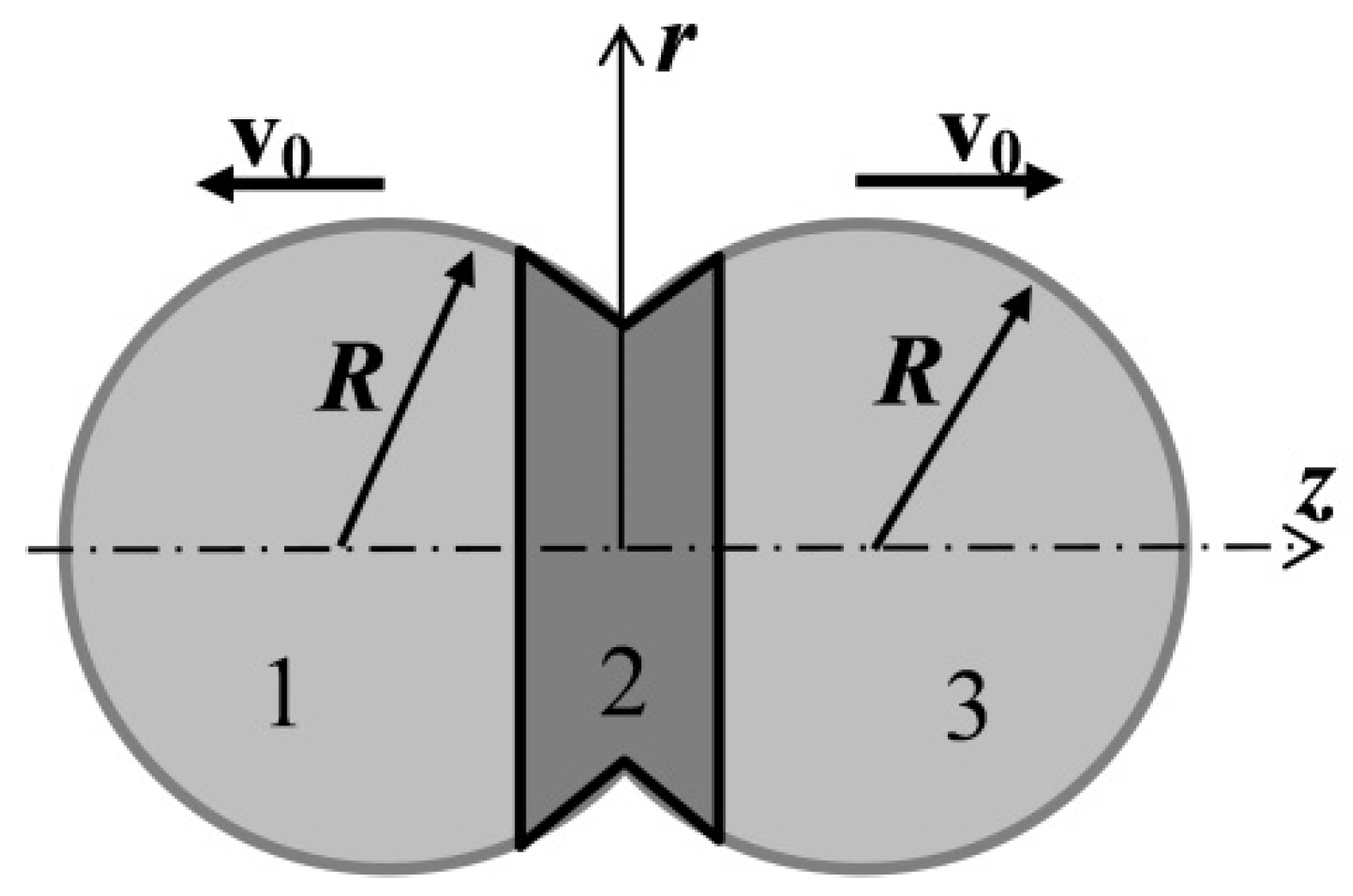
The physical statement of the problem and the schematic of the computational domain are shown in
Figure 1. Two mutually penetrating spherical drops of cytoplasm (non-Newtonian fluid) are located in the external environment. The dimensions of the computational domain were 30·10
−6 × 8·10
−6 m. The radii
R of the drops at the initial moment are equal to 4·10
−6 m. At the initial moment of time, the initial volumes of liquid move as follows: volume 2 is stationary, and volumes 1 and 3 move in opposite directions with the same velocity v
0, equal to 1.2·10
−6 m/s along the axis of symmetry
z. The remaining regions have zero velocity.
Numerical calculations were performed in an axisymmetric statement for a non-Newtonian viscoelastic fluid. The VOF (Volume of Fluid) model was used, in which the liquids are mutually non-penetrating. This model takes into account the surface tension forces at the interface between the liquids. The equations for momentum transfer and continuity in the axial (
z) and radial (
r) directions for this model are as follows [
13]
The relation between the stress and strain rate tensors for a non-Newtonian fluid is as follows (Oldroyd-B model) [
14]:
where
T is the stress tensor,
Tensor
D has the following form
The density
in Equation (1) is calculated using the following equation
where φ
1 are φ
2 are the volume fractions of the external environment and cytoplasm in the computational cell,
is the cytoplasm density, and
is the external environment density.
To compare the numerical results with the experimental data, the parameters of cytoplasm from [
11] were used in the numerical modeling (see
Table 1).
The VOF model used is based on the assumption that the phases under study (in this case, the cell cytoplasm and the external environment) do not interpenetrate. A variable is introduced into the model, which represents the volume fraction of the cytoplasm in the computational cell. In each cell, the sum of the volume fractions of the cytoplasm and the external environment is equal to one. Thus, the values of the variables in any cell determine the current amount of cytoplasm depending on its volume value.
The interface between the cytoplasm and the external environment is determined in accordance with the solution of the continuity equations for the volume fractions of the cytoplasm φ
2 and the external environment φ
1. These equations have the following form:
Here,
Fz and
Fr in Equation (1) are the axial and radial components of the force, respectively, taking into account the surface tension [
15]
where σ is the surface tension at the interface between the cytoplasm and the external environment, and the curvature of the interface
k is determined as follows [
15]
The following boundary conditions were used in the modeling:
The initial configuration of the cytoplasm is specified in the description of the problem statement. The working pressure is taken to be equal to one atmosphere.
Calculations of stress tensors and strain rates for a non-Newtonian fluid according to Equations (2)–(4) were implemented in the form of UDFs (user-defined functions).
The time step of the model was 10−15 s.
Numerical simulations were performed using ANSYS Fluent 6.0.
3. Results of Numerical Modeling
The shape of the cytoplasm surface obtained during modeling for different moments in time is presented in
Figure 2.
When regions 1 and 3 diverge (
Figure 1), the diameter of region 2 decreases under the action of the surface tension force. In this case, an intercellular bridge is formed. With further divergence, the resulting bridge lengthens and becomes thinner. Up to time
t = 60 s, the diameter of the intercellular bridge varies significantly in length. The minimum diameter at this time is located in its middle. At subsequent times, the shape of the bridge becomes almost cylindrical along its entire length. The rate of thinning decreases as the bridge diameter decreases. Having reached the minimum critical diameter (at the time
t = 112 s), the bridge connecting the diverging regions breaks. Subsequently, the remains of the bridge are drawn into the formed volumes under the action of the surface tension force.
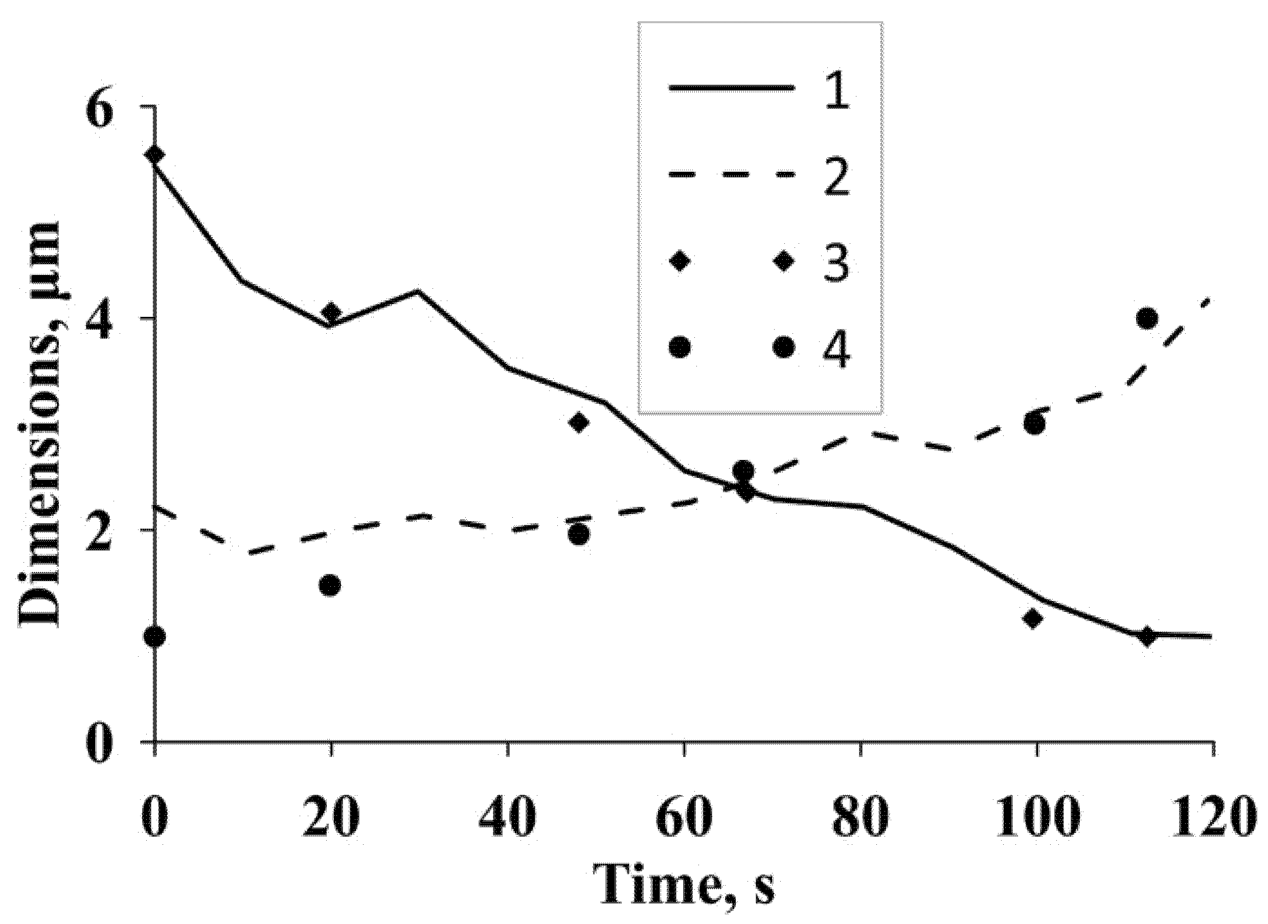
Based on the results of numerical studies, the dependences of the diameter and length of the intercellular bridge on time are plotted in
Figure 3. The same figure shows the experimental dependences from [
11]. The figure shows good agreement between the numerical and experimental results. The calculated and experimental data show that the length and diameter of the intercellular bridge change according to a law that is close to linear.
4. Analytic Analysis
For an approximate qualitative analysis, we consider Equation (2) as an unsteady differential equation with respect to the stress tensor. In this case, we will consider the strain rate tensor as a given function of time
The initial condition for this equation is
For the analytical solution of this equation, we use the method of separation of functions, i.e., we will look for a solution in the following form
Substituting Equation (9) into Equation (11) yields
Since the functions
u and
w are arbitrary, they can be chosen so that the coefficient at
u equals to zero. From here, we have
Next, we substitute Equation (14) into Equation (12) and integrate. This gives
where
C is the integration constant.
The final solution for the stress tensor is
Let us consider two special cases. The first one is when the deformation rates increase according to a linear law
where
A is a constant.
Substitution of Equation (17) into Equation (16) yields the law of variation of stresses over time
where
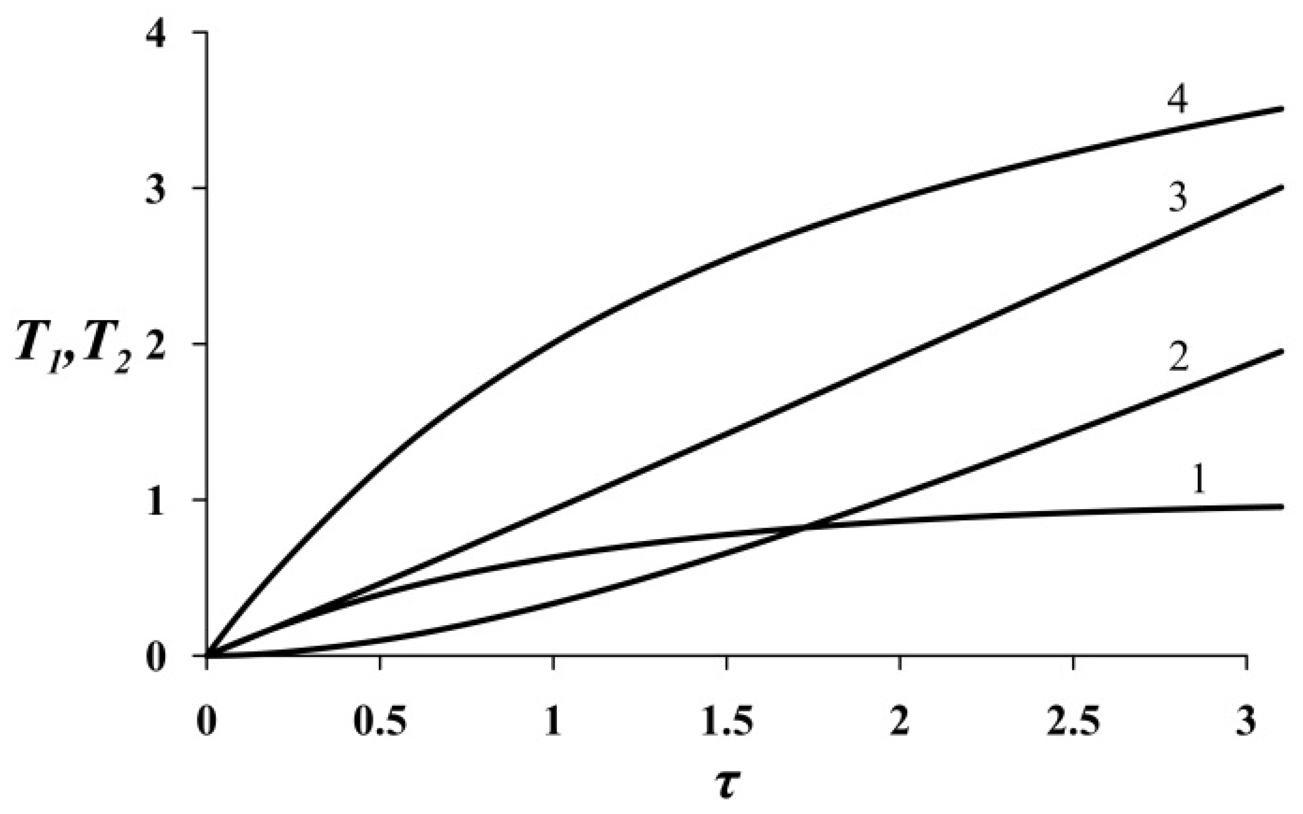
Analysis of Equation (18) shows that the behavior of function
T1 depends on the sign of the value
. If, i.e., when γ > λ, at small values of τ, a sharp increase in stress is observed (curve 4 on
Figure 4); that is, the convexity of the curve is directed upward. This is due to the rapid increase in the deformation rate. Under the condition γ < λ, the opposite picture is observed (curve 2 on
Figure 4). However, at large values of τ, regardless of the value of the parameter
g, the increase in stress is linear. In the case of
, it follows from Equation (18) that the process of cytokinesis obeys a linear law, as shown in curve 3 on
Figure 3. As was said above, according to [
15] the values of the parameters γ and λ tend to equality. Therefore, it is obvious that the most probable scenario of cytokinesis is described by Equation (18) under the condition
, i.e., it is linear.
The second case is when the deformation rates emerges as a Heaviside function
, i.e., instantly,
At the same time,
where
is the Dirac delta function. In this case, solution (15) takes the following form
where
This dependence is also shown in
Figure 4 (curve 1). There is a linear section of increasing stress, after which an asymptote close to the horizontal line appears. Therefore, Equation (21) can describe cytokinesis at an early stage.
5. Conclusions
A homogeneous model of mutually non-penetrating fluids was proposed for the numerical simulation of cytokinesis hydrodynamics, which takes into account surface tension forces at their interface. A viscoelastic non-Newtonian fluid model was used to determine closure relations. This model allows us to trace the formation and rupture of the intercellular bridge that forms during cytokinesis.
Comparison of the numerical simulation results and experimental data [
11] showed their satisfactory agreement. This indicates that the model used adequately describes fluid flow during cytokinesis. The differences in the size of the intercellular bridge at the initial time points are explained by the difference in the initial configuration of the cytoplasm from the real shape of the cell during cytokinesis.
Computational and experimental data show that the length and diameter of the intercellular bridge vary according to a law close to linear, although the properties of the cytoplasm differ from a linear law.
Comparison of numerical and analytical calculations shows that the most probable scenario of cytokinesis can be described by the Oldroyd-B model under the condition
. In this case, the diameter and length of the intercellular bridge change according to a law close to linear, which corresponds to the conclusion of [
15].
In the future, we plan to conduct numerical studies of cytokinesis using other nonlinear models of viscoelastic non-Newtonian fluid.


