Abstract
The accurate classification of cocoa pod ripeness is critical for optimizing harvest timing, improving post-harvest processing, and ensuring consistent quality in chocolate production. Traditional ripeness assessment methods are often subjective, labor-intensive, or destructive, highlighting the need for automated, non-invasive solutions. This study evaluates the performance of R-CNN-based deep learning models—Faster R-CNN and Mask R-CNN—for the detection and segmentation of cocoa pods across four ripening stages (0–2 months, 2–4 months, 4–6 months, and >6 months) using the RipSetCocoaCNCH12 dataset, which is publicly accessible, comprising 4116 labeled images collected under real-world field conditions, in the context of precision agriculture. Initial experiments using pretrained weights and standard configurations on a custom COCO-format dataset yielded promising baseline results. Faster R-CNN achieved a mean average precision (mAP) of 64.15%, while Mask R-CNN reached 60.81%, with the highest per-class precision in mature pods (C4) but weaker detection in early stages (C1). To improve model robustness, the dataset was subsequently augmented and balanced, followed by targeted hyperparameter optimization for both architectures. The refined models were then benchmarked against state-of-the-art YOLOv8 networks (YOLOv8x and YOLOv8l-seg). Results showed that YOLOv8x achieved the highest mAP of 86.36%, outperforming YOLOv8l-seg (83.85%), Mask R-CNN (73.20%), and Faster R-CNN (67.75%) in overall detection accuracy. However, the R-CNN models offered valuable instance-level segmentation insights, particularly in complex backgrounds. Furthermore, a qualitative evaluation using confidence heatmaps and error analysis revealed that R-CNN architectures occasionally missed small or partially occluded pods. These findings highlight the complementary strengths of region-based and real-time detectors in precision agriculture and emphasize the need for class-specific enhancements and interpretability tools in real-world deployments.
1. Introduction
1.1. Context
Cocoa (Theobroma cacao) significantly impacts the economies of small farmers and families worldwide. It is primarily produced in Africa, which accounts for around 75% of the world’s cocoa cultivation, with major producers including the Ivory Coast, Ghana, Cameroon, and Nigeria [1]. In contrast, Latin America’s cocoa production focuses more on fine varieties, contributing about 20% to the global market, particularly from Ecuador and Brazil [1].
In Colombia, cocoa farming provides a livelihood for nearly 35,000 families, and the global demand for cocoa continues to rise. Additionally, in many regions of Colombia, cocoa farming serves as a better alternative to illicit crops like coca leaves. The department of Santander is the leading cocoa producer in the country, accounting for more than 30% of national production.
From an agronomic point of view, to produce fine cocoa, it is important to establish the optimal harvest stage. Farmers must harvest cocoa pods in similar stages of ripeness so that their fermentation process is as homogeneous as possible and thus obtains high-quality derived products [2].
The determination of the state of ripeness in different fruits has been a focus of study in precision agriculture for several decades, and there are research works in the literature that use classification methods based on different characteristics such as color, volatile elements, visible and infrared spectroscopy, fluorescence, and spectral images [3].
It is also important for crops of any type to predict their yields to schedule and plan activities such as fertilization and harvesting, which must be carried out quickly [4,5,6,7,8,9,10,11].
In cocoa crops, different investigations have been carried out to solve the problem of classification into ripeness stages based on various techniques: acoustic signals [12,13]; determination of metabolic profiles through biochemical markers [14]; laser techniques with backscattered images [15]; and physical indicators [2]. These techniques have some limitations for their practical implementation and can be destructive in some cases, so computer vision-based techniques are a lower-cost alternative and possibly more straightforward to implement.
1.2. Challenges in Ripeness Detection
Research on detecting ripeness in various fruits has been growing, highlighting its significance in crop management [16,17,18,19,20,21,22,23,24,25,26]. Most studies concentrate on identifying just two categories: fully ripe and unripe fruits. However, there is a growing body of work aimed at assessing the maturity of different fruits at various stages [3]. Determining the ripeness of fruit at different stages is crucial for making informed agronomic and management decisions in the agribusiness sector.
Detecting different stages of fruit ripeness poses several challenges that can become bottlenecks for research in this area, such as obtaining datasets, using various imaging techniques, light conditions in open fields, and different phenological characteristics that depend on each crop. One of the main challenges is the variability between crops and the characteristics associated with each of these. Each plant has a distinct phenology and specific ways of expressing its maturity. In cocoa, the early stages of ripening are challenging to differentiate by color or size, requiring a texture analysis [27]. In citrus fruits, for example, although color facilitates the classification of ripe and unripe fruits, differentiating between intermediate stages remains complex, especially when the tree has simultaneous ripening stages [28].
A significant challenge in agriculture is identifying fruits in natural or uncontrolled conditions. Factors like varying light levels and the presence of branches, leaves, and other elements can complicate fruit detection by algorithms. For example, in crops such as coffee and citrus, branches or leaves are often mistaken for fruits [28,29]. In some cases, physical characteristics like size or color are insufficient to distinguish between different maturity classes of fruits. This limitation has led to the adoption of more advanced techniques, such as hyperspectral imaging [30]. Although these methods can be costly, they have proven effective in accurately classifying various maturity stages of fruits.
The primary goal of artificial intelligence models in agriculture is to analyze changes and variability in crops, including pest and disease detection, fruit maturity stages, and phenological development among other factors. However, there is still much work to be done. Techniques need to be developed to classify fruits not only based on their ripeness stage but also according to their quality. Additionally, addressing other factors beyond just ripeness classification, such as counting fruits, is crucial for accurately estimating crop yield.
Recent studies in field-oriented research have examined advanced methods that go beyond traditional RGB image-based object detection. For example, Wang et al., in 2025 [31], proposed a geometry-aware 3D point cloud learning method aimed at accurately detecting cutting points in complex field environments. This approach achieved high accuracy despite challenges such as occlusions and unstructured canopies. Although it focused on pruning applications, the study highlights the potential benefits of integrating spatial geometry to enhance object localization in agriculture.
In a similar vein, Wu et al., in 2024 [32], developed an improved CycleGAN framework for detecting pineapples at nighttime. Their work addresses the challenges posed by low-light conditions through image-to-image translation and domain adaptation techniques. This study illustrates how generative models can help mitigate the negative effects of varying lighting conditions, which is also crucial in assessing ripeness in natural open-field environments.
These innovative approaches underscore the importance of exploring advanced vision techniques and non-standard imaging conditions in future research. This aligns with the goal of enhancing cocoa pod detection at various ripening stages in real-world field situations.
This study addresses significant challenges by exploring the use of advanced deep learning models, specifically Faster R-CNN and Mask R-CNN, for the automated detection of cocoa pods at various ripening stages. By utilizing computer vision techniques, we aim to overcome the limitations associated with traditional methods, such as subjectivity, destructiveness, and high costs, while enhancing accuracy in ripeness classification under real-world field conditions. Our approach contributes to finding solutions that meet the need for reliable and noninvasive maturity assessments. It also contributes to the field of precision agriculture by demonstrating the usefulness of these artificial intelligence tools in harvest planning and yield prediction. The findings of this study could contribute to the search for solutions for farmers in optimizing cocoa production and quality, which aligns with the global demand for sustainable and efficient agricultural practices.
Additionally, dataset imbalance, the absence of hyperparameter tuning, and the lack of model interpretability tools are common issues that this work aims to address in its extended experiments.
This paper is organized as follows: Section 2 discusses related works. In Section 3, we present the materials and methods used. Next, Section 4 outlines the results of training the models. Section 5 provides a discussion on the results obtained and explores possible causes. Finally, Section 6 presents the conclusions, limitations, and suggestions for future work.
2. Related Work
Research on ripeness detection can be categorized based on the type of dataset used into two main types:
- Controlled environment datasets: These methods utilize digital image datasets obtained from controlled environments where the fruits have already been harvested [33,34,35,36,37,38,39]. In these cases, the background of the images is free from noise, making classification easier. Algorithms trained using these methods are typically employed in agro-industrial plants for tasks such as fruit classification or packaging.
- Complex environment datasets: in contrast, some models are trained with datasets collected under complex field conditions, where the images are captured before the fruits have been harvested [40,41,42,43,44,45,46,47,48].
This work aims to detect ripeness in cocoa crops under field conditions, which present a complex environment. The goal is to develop algorithms that can identify the ripeness of the cocoa pods before harvest, aiding in yield estimation. Current state-of-the-art classification methods using fruit datasets in complex environments have shown better results with deep neural networks.
Numerous studies in the literature have explored various neural network architectures, with the YOLO family (You Only Look Once) [49,50,51,52,53,54] being one of the most prominent models. This family has demonstrated impressive results in agricultural applications and merits further investigation in this area [24,28,39,41,42,45,55,56,57,58]. However, this work specifically focuses on two widely used models for agricultural solutions: Faster R-CNN [59] and Mask R-CNN [60]. These models have been shown in various studies to possess characteristics that are well-suited for many applications in precision agriculture. Below, we review some of the most significant features of these networks that motivate the interest in using them to detect different stages of maturity in cocoa crops.
2.1. Application of Faster R-CNN and Mask R-CNN in Fruit Ripeness Detection
Convolutional neural network (CNN)-based detection models, particularly Faster R-CNN and Mask R-CNN, have become essential tools for computer vision tasks in precision agriculture, especially in classifying the ripening stages of fruits [3]. These two-stage methods offer significant advantages over traditional techniques. Faster R-CNN is notable for its balance between accuracy and efficiency in object localization [59]. Meanwhile, Mask R-CNN, which builds upon this framework, introduces pixel-level segmentation capabilities that enable precise morphological characterization [60]. However, the application of these models in fruit ripeness presents specific challenges, as documented in the literature. Below, we show some advantages and limitations found in different related works.
2.1.1. R-CNN Models Advantages
High accuracy in detection and localization: R-CNN architectures, especially Faster R-CNN and Mask R-CNN, are known for their high accuracy in object detection and localization [57]. Mask R-CNN is particularly known for accurate target localization and generation of high-quality pixel masks, making it suitable for pixel-level segmentation [61]. In different cases, high accuracies (mAP) have been achieved in the detection/segmentation of various fruits and diseases, such as apple leaf diseases [62], pak choi leaves [61], grapes [63], green fruits [64], tomatoes (even in complex scenarios) [46,65], passion fruit [66,67], peaches [68], strawberries [69], and lychees [70].
Robust and multi-scale feature learning: Convolutional neural networks (CNNs), which serve as the foundation for region-based CNNs (R-CNNs), can automatically extract complex features [71]. Backbone architectures like ResNet address issues such as the gradient vanishing problem in deep networks and effectively learn useful features [68,72]. By integrating Feature Pyramid Networks (FPNs) or similar mechanisms—such as PANet or Multi-Scale Feature Extractors (MSFEs)—we can combine high-level semantic information from deeper layers with low-level fine details from shallower layers. This integration is essential for detecting objects of various sizes in complex scenarios [61,65,67,68]. Additionally, Res2Net, as an enhanced backbone, has demonstrated improved capabilities in multi-scale and high-representation feature extraction [62].
Enhanced spatial localization and segmentation with RoIAlign: RoIAlign is a method that extracts features from regions of interest (RoIs) without rounding their coordinates [60]. It uses interpolation to maintain spatial accuracy, which is key in models such as Mask R-CNN. The RoIAlign layer utilized in Mask R-CNN and improved versions of Faster R-CNN significantly enhances localization accuracy [62]. Unlike RoIPool, which is used in R-CNN and Fast R-CNN, RoIAlign employs bilinear interpolation to map regions of interest to fixed-size feature maps. This approach minimizes inaccuracies caused by quantization [61]. As a result, RoIAlign provides more precise boundaries [46,71] and better captures target boundaries and spatial information. This level of accuracy is particularly crucial for tasks that require high localization precision [71].
2.1.2. R-CNN Models Limitations
Processing (inference) speed: R-CNN models, particularly two-stage architectures like Faster R-CNN and Mask R-CNN, tend to be slower than single-stage detectors such as YOLO [62,73,74]. The original R-CNN was both slow and computationally expensive [75]. While Faster R-CNN does enhance processing speed, it remains slower than YOLOv3 [73,74]. The inference time for Mask R-CNN can also be quite challenging, with reported times of 7.72 s per image for lychees [70] and 1.65 s per tomato [65]. Such inference times can be limiting for real-time applications that require high-speed processing.
Model and training complexity: The original R-CNN featured a complex training process [76]. Two-stage architectures, such as Mask R-CNN, involve multiple interconnected components, leading to increased complexity [60,61]. Additionally, training deeper models, like ResNet101 compared to ResNet50, can significantly extend the training time [61].
Challenges in detecting small objects (on basic architectures): The basic Faster R-CNN may have difficulty detecting small objects because the original RoI Pooling and the Region Proposal Network (RPN) generate features solely from the last convolutional layer. This approach ignores lower-resolution feature maps, which are important for identifying small objects. This issue can be addressed by using multi-scale architectures such as Feature Pyramid Networks (FPN) or Multi-Scale Feature Extraction (MSFE) [67].
Anchor mechanism (for anchor-based models): Although anchors are fundamental in many methods, using them in the Region Proposal Network (RPN) implies tuning complex hyperparameters [73].
In summary, Faster R-CNN and Mask R-CNN are advanced architectures designed for detection and segmentation tasks in computer vision. They are notable for their high accuracy, ability to handle multiple scales, and enhanced spatial localization through the RoIAlign technique. However, adopting these systems involves important trade-offs, including higher computational demands, complexity in training, and limitations in inference speed, especially for real-time applications. The reviewed studies show that while these networks achieve greater accuracy than alternatives like YOLO in complex agricultural scenarios—such as multi-stage fruit ripeness detection and foliar disease segmentation—their practical implementation requires careful consideration of these factors based on the specific needs of the project. Future research could aim to improve their computational efficiency without compromising their robustness, potentially through model compression techniques or hybrid architectures.
On the other hand, computer vision techniques are increasingly being applied to address various challenges in cocoa crops, with many solutions utilizing artificial neural networks (ANNs) [77,78,79,80]. However, there are still relatively few studies focused on classifying the different stages of ripening in cocoa. This work aims to contribute to finding solutions for these challenges.
2.2. Comparison of Two-Stage vs. One-Stage Detectors in Agriculture
Several recent studies have systematically compared two-stage and one-stage object detectors in agricultural contexts, particularly focusing on tasks such as fruit and orchard branch detection.
Sapkota et al., in 2023 [57], evaluated YOLOv8 and Mask R-CNN for instance segmentation in apple orchards. They found that YOLOv8 significantly outperformed Mask R-CNN in both accuracy and speed. YOLOv8 achieved precision and recall rates of 0.90 and 0.95, respectively, for dormant trees, compared to Mask R-CNN’s 0.81 and 0.83 for both metrics [57].
In a study on plum detection, a comparative evaluation of Faster R-CNN (ResNet-101), EfficientDet-D4, RetinaNet, and SSD showed that EfficientDet-D4 achieved the highest accuracy (AP50 = 78.8%) and faster inference time (approximately 12 ms) compared to Faster R-CNN, which had an AP50 of 73.6% and an inference time of around 15.5 ms [81].
Wu et al., in 2024 [82], introduced an improved YOLOv8n model for occluded apple detection, achieving a mean average precision (mAP50) of at least 75.9% in bbox and 75.7% in mask at approximately 44 frames per second (FPS) in complex orchard environments. This performance highlights the robustness and suitability of lightweight one-stage models for real-time applications.
A broader review by Xiao et al. in 2023 [83], analyzed various fruit detection models, including YOLO, SSD, Faster R-CNN, and Mask R-CNN. The findings concluded that one-stage detectors generally offer superior speed, while two-stage detectors tend to provide higher accuracy, particularly in complex conditions involving occlusion and small target sizes [83].
3. Materials and Methods
3.1. Dataset
The RipSetCocoaCNCH12 dataset is the source of data for this work [27]. There are several cultivated varieties of Theobroma cacao, each exhibiting distinct physical characteristics, such as color, fruit shape, yield, and resistance to different diseases. This study centered on the CNCH12 variety grown in Colombia (see Figure 1). CNCH12 was developed by the “Compañía Nacional de Chocolates,” the largest company in the country that transforms cacao into consumer products and is also the biggest purchaser of cacao from farmers.
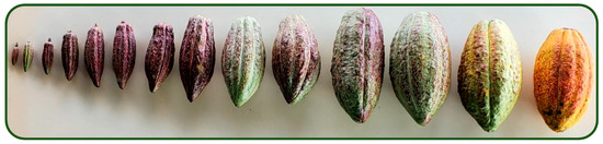
Figure 1.
Cocoa pods of the CNCH12 variety in all stages of development, from 0 to 6 months [27].
The images were collected at the “Compañía Nacional de Chocolates” farm, located in the municipality of Támesis in the department of Antioquia, Colombia (5°43′0″ N–75°41′25″ W). The average elevation of the farm is approximately 1100 m above sea level. This dataset was created between 1 December 2022 and 17 February 2023, which corresponds to the main cacao harvest season in the study area [27].
The dataset consists of four classes representing different ripening stages, starting with the bloom set: (1) Class 1 (0–2 months), (2) Class 2 (2–4 months), (3) Class 3 (4–6 months), and (4) Class 4 (>6 months) (see Figure 2). The dataset can be downloaded from the repository at https://doi.org/10.5281/zenodo.7968315. An additional class corresponding to aborted fruits was originally included in the dataset but has been removed, as it is considered a maturation stage.
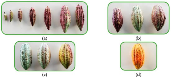
Figure 2.
Ripeness stages: (a) 0–2 months (C1); (b) 2–4 months (C2); (c) 4–6 months (C3); (d) >6 months (C4) [27].
The dataset consists of 4116 images captured on various smartphone models in .JPG format, each with a resolution of 3000 × 3000 pixels. The images are labeled according to the four stages of cocoa ripening, as outlined in Table 1. The initial stage (Class 1) has the highest number of instances, totaling 3427. This abundance can be attributed to the fact that, at this stage, a larger percentage of fruits have just completed the flowering process. During ripening, some fruits may be lost due to pests and diseases, leading to a decrease in quantity as time progresses. Consequently, by the harvest stage, only 1106 instances are available, reflecting the reduced number of images at the later stages. The original dataset included 263 instances of a class labeled “Abortions” (CA). However, this class was removed for this study, as it is not relevant to the ripeness stages.

Table 1.
Quantities in the dataset for each class.
The dataset includes labels in two alternative formats: (1) the COCO 1.0 format, which consists of JSON files for object detection using bounding boxes and polygons, and (2) the Segmentation Mask 1.1 format, which features separate folders for both semantic segmentation and instance segmentation. In this work, we use labels in the COCO format. Examples of images from the dataset are shown in Figure 3 below.
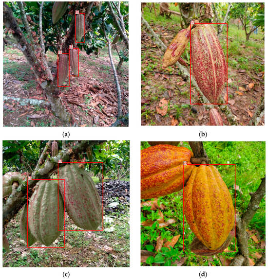
Figure 3.
Examples of labeled images in dataset: (a) c1 (0–2 months); (b) c2 (2–4 months); (c) c3 (4–6 months); (d) c4 (> 6 months).
3.1.1. Data Augmentation and Class Balancing Strategy
During the training data preparation process, it was identified that the dataset exhibited an imbalance in the distribution of the target categories, particularly for the classes labeled as c2, c3, and c4. Such imbalance can negatively impact the performance of detection and segmentation models, especially by reducing their ability to correctly identify underrepresented classes.
To address this issue, a selective data augmentation strategy was implemented. This process involved generating synthetic variations of the existing images while preserving their associated annotations. The objective was to increase the number of training instances for underrepresented categories without the need to collect additional data.
The number of augmentations applied to each image was determined based on the relative scarcity of each class within the training set. Specifically, a variable number of augmented images was generated according to the categories present in each image. The specific augmentation criteria were as follows:
- -
- If an image contained class c2, 1 additional augmented image was generated.
- -
- If it contained class c3, 1 additional augmented image was generated.
- -
- If it contained class c4, 2 additional augmented images were generated.
This procedure was formalized through an algorithm that iterates over all images in the original dataset and, depending on the classes present in each image, accumulates a counter indicating the number of augmentations to be applied. The following augmentation techniques were applied using the Albumentations library:
Horizontal flip randomly flips the image along the horizontal axis with a probability of 0.5. This transformation is commonly used to increase the variability of object positions within the dataset.
Vertical flip randomly flips the image along the vertical axis with a probability of 0.5. Although less frequent in natural scenes, this operation can be beneficial in agricultural and aerial imagery where objects may appear in diverse orientations.
Random brightness and contrast adjustment modifies the brightness and contrast of the image within a random range with a probability of 0.5. This technique helps the model to generalize better under varying lighting conditions.
Rotation rotates the image by a random angle within the range of −20 to +20 degrees, with a probability of 0.5. This operation increases the robustness of the model to rotated instances of objects.
The impact of this augmentation strategy is shown in Figure 4, which displays the class distribution after augmentation. A more balanced distribution was achieved, with an increased presence of previously underrepresented classes such as c2, c3, and c4, reducing the dominance of class c1 from 42.2% to 25.7%. This adjustment improves the representativeness and balance of the dataset, contributing to the development of more reliable and generalizable deep learning models for object detection and segmentation tasks.

Figure 4.
Impact of the selective data augmentation strategy (a) before applying data augmentation and (b) after applying data augmentation.
3.1.2. Dataset Partitioning After Data Augmentation
Following the data augmentation process, the resulting dataset was cleaned and partitioned into three subsets, training, validation, and testing, based on the total number of annotated instances for the relevant target classes (c1, c2, c3, and c4). The distribution of annotations was designed to ensure a representative and balanced split for model development and evaluation. Specifically, 70.39% of the total annotations were assigned to the training set, 19.62% were allocated to the validation set, and 9.99% were reserved for the test set (Figure 5).
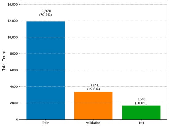
Figure 5.
Total instance counts and percentages per subset.
This stratified distribution ensures that the training set contains most of the annotated data for effective model learning, while preserving sufficient samples in the validation and test sets to allow for robust performance evaluation and hyperparameter tuning. Importantly, this split was calculated based solely on the annotated instances of the four target classes.
Figure 6 shows the final distribution of annotated instances per class (c1 to c4) across the training, validation, and test sets. The training set contains the highest number of annotations for each class, ensuring sufficient data for learning, while validation and test sets maintain a consistent and proportional representation. Class c2 is the most frequent across all subsets, followed by c1, c3, and c4. This balanced distribution helps ensure that the model is trained and evaluated fairly across all target categories.
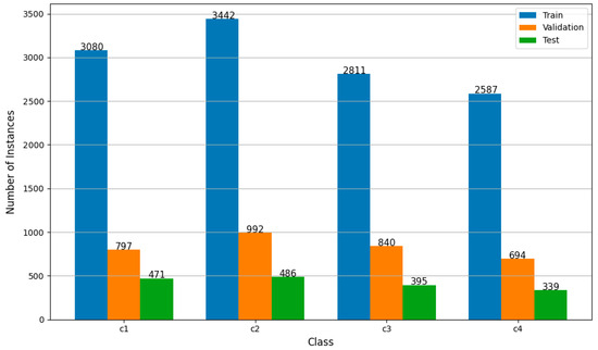
Figure 6.
Instance distribution per subset and class.
3.2. Convolutional Neural Networks Selected for This Research
Convolutional neural network (CNN)-based object detection architectures have transformed the field of computer vision. The first R-CNN model, which stands for Regions with CNN Features, was introduced in 2014 by Ross Girshick and his colleagues in their paper titled “Rich Feature Hierarchies for Accurate Object Detection and Semantic Segmentation” [76]. This landmark work marked a significant turning point in object detection by integrating region proposals (RP)—inspired by algorithms like selective search—with CNN-based feature extraction. This approach replaced traditional manual descriptors like SIFT or HOG, paving the way for more accurate detection methods.
The original R-CNN model inspired a new generation of models when its limitations, such as slow processing due to the independent handling of regions, became apparent. As a result, subsequent advancements led to the development of Fast R-CNN [84], Faster R-CNN [59], and Mask R-CNN [60]. These improvements have significantly impacted practical applications, particularly in areas where precision is crucial, such as precision agriculture (for fruit and pest detection), self-driving technology (for pedestrian and vehicle detection), and medicine (for medical image analysis). In this work, we utilized the enhanced versions, Faster R-CNN and Mask R-CNN.
3.2.1. Faster R-CNN
This model advances the integration of RP generation directly within the neural network through a “Region Proposal Network (RPN)” [85]. A summary of its architecture is presented in Figure 7, below.
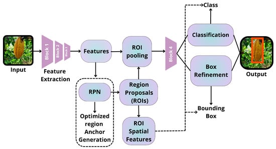
Figure 7.
Architecture summary of Faster R-CNN [59].
The RPN utilizes a sliding window technique on the convolutional feature map to generate region proposals known as “anchors.” At each location of the window, the RPN predicts several proposals, typically defaulting to nine anchors with various scales and aspect ratios [59].
Once the anchors are generated, they undergo evaluation by a classification layer, which determines whether they contain an object, and a regression layer, which refines the bounding box coordinates [59]. The RPN is trained in an end-to-end manner and shares convolutional layers with the Fast R-CNN detection network, which significantly enhances speed without compromising accuracy.
Despite being faster, this model’s two-stage architecture can be slower compared to single-stage detectors such as YOLO and SSD [86]. It may also struggle with detecting very small objects [87]. Additionally, spatial misalignment stemming from RoI pooling remains an issue in the base Faster R-CNN architecture [60].
3.2.2. Mask R-CNN
Mask R-CNN extends Faster R-CNN by adding a third branch to predict pixel-level segmentation masks for each RoI (region of interest) [88,89]. A summary of its architecture is presented in Figure 8, below.
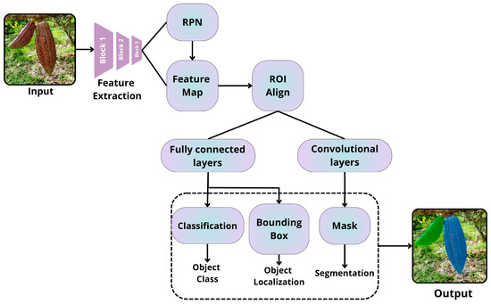
Figure 8.
Architecture summary of Mask R-CNN [60].
A key innovation of Mask R-CNN is the introduction of “RoIAlign.” This technique addresses the spatial misalignment issues caused by quantization in “RoIPool,” which is used in Fast R-CNN and Faster R-CNN. RoIAlign employs bilinear interpolation to compute feature values at precise sampling locations within each RoI bin, resulting in more accurate segmentation masks [88]. This model not only detects objects and localizes their boundaries with bounding boxes but also provides pixel-level instance segmentation.
Moreover, RoIAlign significantly enhances the accuracy of segmentation masks compared to methods that use RoIPooling [60]. As a result, this network can tackle more complex tasks beyond simple object detection, such as identifying image tampering by segmenting forged regions [89].
However, the limitations of this model include its complexity compared to Faster R-CNN due to the addition of the mask branch. This complexity results in a higher computational burden, although the overhead is relatively small—approximately 20% more than Faster R-CNN [60].
In summary, the R-CNN family has evolved significantly to enhance both accuracy and efficiency in object detection. The original R-CNN was groundbreaking but slow. Fast R-CNN improved the speed by processing the image only once, though it still depended on external region proposals. Faster R-CNN made a major advancement by integrating proposal generation directly into the network, achieving near-real-time speeds. Finally, Mask R-CNN expanded its functionality to include instance segmentation, offering more detailed information about detected objects, albeit with increased computational complexity. Each iteration has built upon the previous one, addressing its limitations while introducing new capabilities.
3.3. Detectron2 Library
For this research, we used the Detectron2 library. Detectron is a computer vision library developed by Facebook AI Research that focuses on object detection, instance segmentation, and various advanced tasks. Its successor, Detectron2, is an enhanced and more flexible version written in PyTorch version 2.6.0+cu124. Detectron2 offers state-of-the-art models such as Faster R-CNN, Mask R-CNN, RetinaNet, and Cascade R-CNN, among others.
Detectron2 builds upon the original Detectron, which was based on Caffe2, and has transitioned to PyTorch to provide better flexibility and performance. Its modular design enables the integration of modern backbones like ResNeXt and Swin Transformer, as well as advanced techniques such as ROIAlign and Feature Pyramid Networks (FPNs).
Nomenclature in Detectron2
The nomenclatures in Detectron2 follow a pattern that indicates the model architecture, backbone, training configuration, and network characteristics. Here is a detailed explanation of each one:
Naming Convention Structure:
faster_rcnn_<BACKBONE>_<NECK>_<TRAINING-SCHEDULE>
- faster_rcnn: Base architecture (Faster R-CNN).
- BACKBONE: Feature extraction backbone (e.g., R_50, X_101_32x8d).
- NECK: Neck design for multi-scale feature handling (e.g., C4, FPN, DC5).
- TRAINING-SCHEDULE: Training duration/hyperparameters (e.g., 1x, 3x).
Key components explained:
Backbones
- ✓
- R_50: ResNet-50 (50 layers).
- ✓
- R_101: ResNet-101 (101 layers, deeper/more accurate).
- ✓
- X_101_32x8d: ResNeXt-101 with 32 groups and 8 bottleneck width (higher capacity than ResNet).
Neck
- ✓
- C4: Uses conv4 features for RPN and ROI heads.Pros: Faster but less precise for small objects.
- ✓
- FPN: Feature Pyramid Network (multi-scale features).Pros: Best for objects of varying sizes (e.g., fruits at different distances).
- ✓
- DC5: Dilated convolutions in conv5 (higher spatial resolution).Pros: Better for small objects but computationally heavy.
Training Schedule
- ✓
- 1x: Standard training (~90k iterations).
- ✓
- 3x: Extended training (~270k iterations).
- ✓
- Pros: Higher accuracy but 3× slower.
3.4. Metrics
In computer vision, the rigorous evaluation of detection and segmentation models requires metrics that assess not only spatial accuracy but also consistency under varying conditions such as scale, occlusion, and annotation quality. In this work, we utilize standard metrics like mean average precision (mAP), AP50, and AP75, which are widely accepted in the literature (e.g., COCO and Pascal VOC) for their effectiveness in quantifying the trade-off between recall and precision across multiple Intersection over Union (IoU) thresholds.
3.4.1. Intersection over Union
Intersection over Union (IoU) is a key metric used in object detection and segmentation to measure the accuracy of a prediction in comparison to a ground-truth annotation. It is calculated by taking the ratio of the area of overlap (the intersection) between the predicted bounding box or mask and the ground-truth annotation, to the total area covered by both the predicted and ground-truth areas (the union) [90].
3.4.2. Average Precision
The average precision (AP) metric is essential for assessing detection and segmentation models in realistic, non-iconic environments, like those found in the COCO dataset. AP combines precision (the accuracy of predictions) and recall (the ability to detect all relevant objects), providing a balanced measure of performance in complex scenarios [91]. These scenarios can include situations where objects are occluded, set against chaotic backgrounds, or viewed from non-standard perspectives. Standard thresholds: 0.5 (AP50) and 0.75 (AP75). An IoU ≥ 0.5 is a valid detection in most benchmarks (e.g., COCO) [91].
The mAP is the average of the sum of the average precisions (APs) for each class:
where:
n: number of classes;
k: k-th prediction;
: average precision per class;
AP50: evaluates with a minimum IoU of 0.5 (“good enough” detections);
AP75: requires higher spatial precision (IoU ≥ 0.75), relevant for critical applications.
Standardizing the use of average precision (AP) across various thresholds enables fair comparisons between different architectures. This method encourages the development of models that can generalize well under real-world conditions, balancing both accuracy and adaptability [91].
3.5. Model Configuration and Training Parameters for Base Line
This study assessed the Faster R-CNN and Mask R-CNN models, implemented using configurations based on pre-trained architectures from the COCO Model Zoo. We chose all models that were preconfigured in the library.
We applied transfer learning by initializing the model weights with the pre-trained values from COCO and adjusted only the classification layer (ROI head) to accommodate the five classes of our custom dataset (NUM_CLASSES = 5). The training was set up with a base learning rate of 0.001, a batch size of 2 images per GPU (IMS_PER_BATCH = 2), and a maximum limit of 2500 iterations (MAX_ITER) to optimize the balance between stability and computational efficiency.
To manage regions of interest (RoIs), we defined a batch size of 128 instances per image (BATCH_SIZE_PER_IMAGE), ensuring speed while maintaining accuracy in small detection scenarios. Validation was conducted every 50 iterations (EVAL_PERIOD = 50) using a separate validation dataset.
Detectron2 utilizes the Stochastic Gradient Descent (SGD) optimizer with momentum by default. This configuration involves a momentum value of 0.9 and an L2 weight decay (regularization) of 0.0001. The SGD optimizer was chosen for its effectiveness in computer vision tasks, particularly when working with pre-trained models on extensive datasets like COCO. The momentum helps accelerate convergence by smoothing gradient updates in consistent directions, while weight decay prevents overfitting by penalizing large weights in the network. The base learning rate is set at 0.001 and remains untuned to prioritize training stability due to the use of transfer learning. Although SGD is the default option, Detectron2 provides the flexibility to implement other optimizers, such as Adam. However, for this initial experiment, the standard configuration was followed. Finally, the original dataset without balancing was split into 70% for training, 20% for validation, and 10% for testing.
3.6. Hyperparameter Optimization
Hyperparameter optimization is a crucial step in enhancing model performance for deep learning applications, especially when deploying pre-trained architectures on custom datasets that have specific domain constraints. In this study, we utilized Bayesian optimization through the scikit-optimize (skopt) library to efficiently navigate the hyperparameter search space of the two best-performing models identified in our baseline experiments: Faster R-CNN X-101-32x8d-FPN-3x and Mask R-CNN X-101-32x8d-FPN-3x.
We selected Bayesian optimization over grid search and random search because it can model the underlying objective function using probabilistic surrogate models, such as Gaussian processes [92,93]. This method strategically balances exploration and exploitation through an acquisition function. As a result, it typically requires fewer iterations to converge on an optimal or near-optimal set of hyperparameters, making it computationally efficient for time-consuming training processes associated with deep convolutional architectures.
3.7. Confidence Heatmaps for Object Detection
In the context of precision agriculture, accurate and interpretable object detection is essential for supporting automated phenotyping, yield estimation, and decision-making systems. In this study, we implemented confidence heatmaps as an additional interpretability tool to assess how the Faster and Mask R-CNN models spatially distribute their confidence over cacao pod predictions. This visualization was particularly valuable for identifying detection gaps in heterogeneous field conditions, such as occlusions by branches or leaves, lighting variability, and varying fruit maturity stages. By observing where the model assigns high or low confidence, we were able to better understand its behavior, especially in complex visual scenes. This insight is crucial in agricultural environments, where undetected or misclassified fruits can significantly impact productivity measurements. Thus, incorporating confidence heatmaps helped guide improvements in dataset balancing, model optimization, and post hoc error analysis, ultimately contributing to the robustness and transparency of AI tools used in precision agriculture. Areas with high overlap between bounding boxes and elevated confidence values result in more intense heatmap regions, typically displayed in warmer colors (e.g., red or orange). Conversely, areas with low confidence appear in cooler tones (e.g., blue or green).
This method serves both diagnostic and interpretative purposes. It allows us to achieve the following:
- Identify missed detections—regions with visible objects but low or no heat response;
- Assess the spatial uncertainty of predictions;
- Evaluate potential confusion between classes in ambiguous contexts.
This technique draws inspiration from earlier work on visual explanations for deep learning models in classification and detection tasks. Similar heatmap-based methods have been widely adopted for interpreting convolutional neural networks (CNNs), notably in the work of Zhou et al. in 2016 [94], who introduced Class Activation Mapping (CAM), and later by Selvaraju et al. in 2017 with Grad-CAM [95]. However, those methods typically focus on class relevance in feature maps rather than detection confidence per region.
4. Results
4.1. Baseline Results
4.1.1. Top Performer Selection: Comparative Analysis of the Four Models with the Highest mAP in Faster R-CNN and Mask R-CNN
Table 2 presents the four best models evaluated in the experiment with the original dataset (without data augmentation or balancing), comparing the performance of the Faster R-CNN and Mask R-CNN architectures under various configurations. The table summarizes key metrics, including the mean average precision (mAP) and average precisions (APs) at 50% and 75% Intersection over Union (IoU) thresholds, along with performance categorized from c1 to c4. The results indicate that the Faster_R_CNN_X_101_32x8d_FPN_3x variant achieved the highest mAP of 64.145, outperforming the other models across most metrics. Additionally, it is noted that configurations utilizing ResNeXt-101 (X_101) generally perform better than those based on ResNet-50 (R_50), highlighting the considerable influence of the backbone architecture on model performance. The detailed values obtained are listed below:
Table 2.
Top four models ordered from highest to lowest performance.
The attached graphs (Figure 9, Figure 10, Figure 11 and Figure 12) illustrate the evolution of average precision and loss during the training of the top-performing models in the experiments with Faster R-CNN and Mask R-CNN. Figure 6 and Figure 8 show the trend of the average precision metric for the two best models of each architecture, demonstrating stable convergence in models with more complex backbones (e.g., X_101_32x8d_FPN).
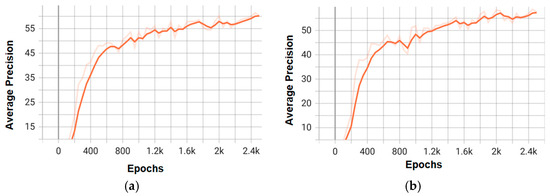
Figure 9.
Training graphs of average precision for the top two models of the Faster RCNN architecture: (a) faster_rcnn_X_101_32x8d_FPN_3x; (b) faster_rcnn_R_50_C4_3x.
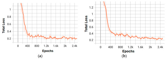
Figure 10.
Training loss graphs for the three best models of the Faster RCNN architecture: (a) faster_rcnn_X_101_32x8d_FPN_3x; (b) faster_rcnn_R_50_C4_3x.
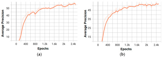
Figure 11.
Training graphs of average precision for the top two models of the Mask RCNN architecture: (a) mask_rcnn_X_101_32x8d_FPN_3x; (b) mask_rcnn_R_50_DC5_3x.
Figure 12.
Training loss graphs for the top two models of the Mask RCNN architecture: (a) mask_rcnn_X_101_32x8d_FPN_3x; (b) mask_rcnn_R_50_DC5_3x.
On the other hand, Figure 10 and Figure 12 detail the gradual reduction of loss during training, indicating effective optimization, especially in configurations like faster_rcnn_X_101_32x8d_FPN_3x (Figure 9a), which exhibits a smoother curve compared to lower-capacity models (e.g., R_50).
These graphs not only validate the superior performance of the X_101 variants—consistent with the mAP values—but also highlight the differences in convergence speed and stability between the architectures. Combining these visualizations with the tabular data provides a comprehensive understanding of the trade-offs between accuracy and efficiency for each model.
4.1.2. Comprehensive Performance Evaluation: Comparative Metrics of mAP, AP50/75, and Specific Categories in Faster R-CNN and Mask R-CNN Models
Table 3 and Table 4 provide a detailed performance analysis of the Faster R-CNN and Mask R-CNN architectures on the test set, respectively. These tables compare various model configurations, emphasizing key metrics such as mAP, AP50 (precision at a 50% IoU threshold), AP75 (precision at a 75% IoU threshold), and performance across different categories (c1 to c4).
Table 3.
Results of the average precision metric on the test set for each Faster-RCNN network.
Table 4.
Results of the average precision metric on the test set for each Mask-RCNN network.
In Table 3, which focuses on Faster R-CNN, the best model, named faster_rcnn_X_101_32x8d_FPN_3x, stands out with an mAP of 64.145%. This performance significantly surpasses that of configurations based on ResNet-50 (R_50), highlighting the advantages of more complex backbone architectures, such as ResNeXt-101. Additionally, it is evident that models trained with 3x training schemes (longer training duration) generally outperform those trained with 1x schemes. For example, faster_rcnn_R_50_C4_3x achieved an mAP of 60.360%, compared to faster_rcnn_R_50_C4_1x, which had an mAP of 59.820%.
Table 4, which focuses on Mask R-CNN, indicates that the model mask_rcnn_X_101_32x8d_FPN_3x achieves the highest mean average precision (mAP) of 60.812%. This result is closely followed by the mask_rcnn_R_50_DC5_3x model, which has an mAP of 59.875%. Notably, the mask_rcnn_R_50_DC5_3x model excels in specific categories, achieving an impressive 89.419% in the c4 category, even surpassing the X_101 model in this metric. These findings suggest that while more advanced backbone architectures generally enhance overall performance, certain configurations can be optimized for specific categories.
The initial evaluation results revealed noticeable performance differences across models, particularly in the detection of specific classes (e.g., c2 and c3). While the model faster_rcnn_X_101_32x8d_FPN_3x achieved the highest overall mAP (64.15%) and strongest class-level performance (notably 92.42% AP in C4), the relatively lower scores in classes c2 and c3 indicated potential imbalances affecting the learning process. These findings motivated a more in-depth investigation including class-specific data balancing, Bayesian hyperparameter optimization, and a comparative evaluation using YOLOv8-based architectures to explore improvements in accuracy, robustness, and class-level fairness.
4.2. Enhanced R-CNN Models with Balancing and Tuning
In this study, we focused on two key hyperparameters for the Bayesian optimization process: the learning rate (lr) and the optimizer. This choice was made because both parameters significantly impact the training process and the generalization capability of detection models such as Faster R-CNN and Mask R-CNN. By properly tuning these two factors, we can achieve substantial performance improvements without having to alter more structural aspects of the models. The search space for Bayesian optimization was defined based on two selected hyperparameters, which were chosen as follows:
Learning rate (lr): This parameter was sampled from a log-uniform continuous distribution in the range [1 × 10⁻⁵, 1 × 10⁻³]. The use of a log-uniform prior allows finer exploration of small values, which are often critical for stable convergence in deep neural networks.
Optimizer: This categorical hyperparameter included three widely used options: SGD, Adam, and AdamW. Each optimizer brings distinct convergence properties and regularization effects, making it essential to evaluate their impact within the optimization process.
This design allowed the optimizer to explore both continuous and categorical variables in a compact yet representative space, balancing expressiveness and computational feasibility.
While there are other important hyperparameters to consider, such as batch size, non-maximum suppression (NMS) thresholds, and the number of Region Proposal Network (RPN) proposals, including them would have greatly expanded the search space and increased the computational complexity of the experiment beyond the scope of this work. We believe that these additional factors can be explored in future studies.
The optimization was conducted solely on the two architectures that demonstrated the best initial performance during the base training sessions: faster_rcnn_X_101_32x8d_FPN_3x and mask_rcnn_X_101_32x8d_FPN_3x. Below, we present the results of the Bayesian search, including the evolution of the objective function and the distribution of the evaluated combinations.
In total, twenty evaluations of the search space were conducted, as demonstrated in the convergence graph below. This visualization illustrates how the optimization process was effectively directed toward the best-performing areas of the space.
Figure 13 summarize the results of the Bayesian hyperparameter optimization performed on the faster_rcnn_X_101_32x8d_FPN_3x model. The search focused on two key parameters, the learning rate (lr) and the optimizer, as they are known to have a critical influence on convergence speed and generalization performance in deep convolutional detection architectures.
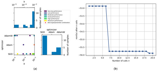
Figure 13.
Bayesian hyperparameter optimization for Faster R-CNN X-101-32x8d-FPN-3x: (a) search space exploration and performance distribution; (b) convergence curve of the optimization process.
Figure 13a presents the relationship between the learning rate (lr), optimizer type, and model performance as evaluated during Bayesian optimization. Each point in the central plot corresponds to a specific configuration of hyperparameters (optimizer × learning rate), colored by performance level (e.g., from “very low” to “maximum” performance). The red star indicates the best-performing combination, which corresponded to Adam with a learning rate of approximately 1 × 10⁻³. The histograms show that most of the search iterations concentrated around higher learning rates and favored SGD over other optimizers.
The red star marks the best configuration found, which corresponds to a learning rate of 1 × 10⁻³ and the Adam optimizer. Notably, although the SGD optimizer was frequently sampled, the best results were consistently obtained using Adam, reinforcing its suitability for this model when paired with an appropriately tuned learning rate.
Figure 13b shows the convergence plot of the Bayesian optimization process over 20 iterations. The y-axis represents the best (lowest) value of the objective function found up to that iteration (in this case, the negative mAP, since the optimization process minimizes the function). The clear drop after iteration 6 indicates a rapid improvement in performance once a promising region of the search space was found. From iteration 7 onward, the function stabilizes, showing convergence around a minimum value, which corresponds to the configuration identified as optimal.
Together, these results not only identify a strong hyperparameter setting for the model but also illustrate the utility of Bayesian optimization in efficiently guiding hyperparameter tuning. These findings provided the foundation for further comparative experiments including other hyperparameters and final model training.
Figure 14a shows the Bayesian hyperparameter optimization space applied to the mask_rcnn_X_101_32x8d_FPN_3x model. There is a noticeable concentration of tests around a learning rate of 1 × 10⁻³ using the Adam optimizer, indicating that the search algorithm found these combinations to be promising. However, the best result was achieved with the SGD optimizer and a learning rate of 0.001. This reinforces the importance of systematically exploring the hyperparameter space, even in less frequently tested regions.
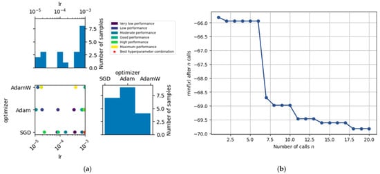
Figure 14.
Bayesian hyperparameter optimization for Mask R-CNN X-101-32x8d-FPN-3x: (a) search space exploration and performance distribution; (b) convergence curve of the optimization process.
Figure 14b displays the convergence behavior of the Bayesian optimization process applied to the Mask R-CNN architecture. The curve represents the best value of the objective function (in this case, the negative mAP) found up to each iteration.
Initially, during the first six evaluations, the performance remained relatively flat, indicating that the configurations tested in the early phase did not yield significant improvements. However, a sharp drop occurred around iteration 7, where the optimizer identified a region of the hyperparameter space (specifically involving a higher learning rate and the SGD optimizer) that resulted in a notable increase in model performance.
4.3. Comparative Performance Analysis of Faster R-CNN, Mask R-CNN, and YOLOv8
In recent years, YOLO (You Only Look Once) models have emerged as a leading choice for real-time object detection due to their speed, efficiency, and high accuracy. This is especially true in various applications, including those in agriculture. Comparing R-CNN architectures with the latest YOLOv8 models is crucial not only for quantifying performance differences but also for understanding the trade-offs between detection accuracy and computational costs. This comparison is particularly relevant in agricultural settings, where deployments may involve edge devices, UAVs, or mobile platforms with limited resources.
4.3.1. Training Configuration for Faster R-CNN and Mask R-CNN
For the Faster R-CNN X-101-FPN architecture, transfer learning was performed starting from COCO-pretrained weights. To maintain a balance between generalization and task-specific learning, only the initial two convolutional blocks of the backbone were frozen (i.e., FREEZE_AT = 2), preserving foundational visual features while allowing the deeper layers to adapt to cacao pod detection.
The training was performed using the Adam optimizer, which was selected based on results from Bayesian hyperparameter optimization. The learning rate was set to 0.001, with standard β1 = 0.9 and β2 = 0.999 values. No learning rate decay (SOLVER.STEPS = []) was applied, allowing the optimizer to maintain a consistent update rate throughout the training process. A weight decay of 0.0001 was used to regularize learning.
The training ran for 5000 iterations, with a batch size of 8 images and 128 sampled ROIs per image during the ROI training phase. No early stopping was applied, but performance on the validation set was monitored periodically.
For the Mask R-CNN X-101-FPN model, a partial fine-tuning approach was implemented to balance generalization and specialization. Specifically, the first two residual blocks of the backbone network were frozen to retain general visual features, while the deeper layers remained trainable to capture task-specific patterns. Additionally, the proposal generator (RPN) and feature extraction components of both the bounding box and mask heads were also frozen. This strategy was intended to reduce overfitting, accelerate convergence, and limit the number of trainable parameters in the early training stages.
The model was optimized using Stochastic Gradient Descent (SGD) with a momentum of 0.9. The learning rate, determined via Bayesian optimization, was fixed at 0.001 throughout training. No learning rate decay or scheduling was applied during the 5000 iterations of training. Evaluation was performed every 200 iterations on the validation set to monitor learning progression.
A batch size of 8 images and 128 proposals per image were used during training. The total number of classes in the detection and segmentation heads was set to five, corresponding to the annotated categories in the cacao dataset. Although no explicit early stopping criterion was enforced, the evaluation frequency allowed continuous monitoring and ensured that training could be manually halted if overfitting was observed.
4.3.2. Training Configuration for YOLOv8
To ensure a fair comparison with the R-CNN models, the YOLOv8x and YOLOv8l-seg architecture—comparable in size and complexity to Faster and Mask R-CNN X-101—was trained under similar hyperparameter conditions. The model was initialized with COCO-pretrained weights (yolov8x.pt) and fine-tuned using the cacao pod dataset.
The training was conducted over 100 epochs, approximately equivalent to 5000 iterations in the Detectron2 framework, assuming a batch size of 8. Key hyperparameters were aligned with those used in the R-CNN models: the initial learning rate was set to 0.001, the batch size was 8, and Adam was used as the optimizer with a weight decay of 0.0001. These values mirror the configuration applied in both Faster and Mask R-CNN setups.
To control overfitting and speed up convergence, the first 10 layers of the YOLOv8 backbone were frozen (freeze = 10), a practice analogous to freezing the first two blocks in the Detectron2 configurations (FREEZE_AT = 2). The input resolution was set to 640 × 640 pixels, ensuring consistency with common YOLOv8 benchmarks and maintaining a good trade-off between speed and accuracy.
All training outputs and logs were saved to a designated project directory for reproducibility and further analysis. This configuration allows direct comparison with R-CNN-based approaches, providing insight into the relative strengths of real-time detection architectures in the context of precision agriculture and cacao pod phenotyping.
4.3.3. Comparative Performance of R-CNN and YOLOv8 Models
Table 5 presents a comprehensive evaluation of four models—YOLOv8x, YOLOv8l-seg, Faster R-CNN X-101-32x8d-FPN-3x, and Mask R-CNN X-101-32x8d-FPN-3x—based on average precision (AP) metrics across the complete test set and per class (C1 to C4). YOLOv8x, a high-capacity detection model, achieved the best overall results with a mean average precision (mAP) of 86.36%, AP50 of 91.80%, and AP75 of 90.68%. It demonstrated outstanding per-class performance, particularly in classes C3 (91.52%) and C4 (94.90%). Despite its strong performance, class C1 showed a comparatively lower AP (69.60%), likely due to small object size or class imbalance—an issue observed across all models.
Table 5.
Comparative performance of R-CNN and YOLOv8 models on the test subset.
YOLOv8l-seg, the segmentation variant, showed slightly lower performance in mAP (83.86%) and AP50 (88.22%) compared to YOLOv8x. However, it achieved superior performance in class C4 (95.60%) and comparable results for C2 (87.00%) and C3 (89.00%). Interestingly, it had the lowest AP for C1 (55.30%), reinforcing the challenge in detecting smaller or less distinct instances of this class using segmentation architectures.
Faster R-CNN X-101-32x8d-FPN-3x, although a strong baseline in the R-CNN family, underperformed compared to YOLO models with an mAP of 67.75%. The model particularly struggled with class C1 (45.66%), suggesting limitations in detecting small or occluded pods. Still, it performed reasonably in C4 (84.19%) and showed solid AP50 (82.23%), indicating that it can detect objects at lower IoU thresholds effectively.
Mask R-CNN X-101-32x8d-FPN-3x, designed for instance segmentation, outperformed its detection-only counterpart in all metrics, with an mAP of 73.21% and stronger scores across C2 (70.55%), C3 (79.07%), and C4 (92.63%). Its class C1 performance (47.31%), although better than Faster R-CNN, remained lower than YOLOv8x, confirming persistent detection challenges for this category.
The comparative analysis reveals that YOLOv8x consistently achieves the highest overall and per-class precision, outperforming all other models. Instance segmentation architectures—particularly YOLOv8l-seg and Mask R-CNN—show strong performance on class C4, likely due to the clearer boundaries of mature cacao pods. However, all models struggle with class C1, possibly due to its small size, visual blending with the background, or class imbalance, indicating a need for targeted augmentation or advanced feature extraction. Notably, Mask R-CNN outperforms Faster R-CNN, underscoring the added value of segmentation capabilities in complex agricultural imagery. These findings emphasize the robustness of real-time detectors like YOLOv8 and motivate further research into segmentation-based improvements and class-specific refinements.
Figure 15 shows average precision curves during training. The training curves reveal that YOLOv8x achieved the highest and most stable average precision (~0.89), converging rapidly and consistently, followed closely by YOLOv8l-seg (~0.86), which also showed smooth progression despite minor early fluctuations. In contrast, Faster R-CNN reached a final AP of ~70 but exhibited greater variability throughout training, while Mask R-CNN showed more stable learning, converging around ~66. These results indicate that YOLOv8 models not only train more efficiently but also outperform R-CNN architectures in this task, though Mask R-CNN offers robust and consistent learning, making it suitable for complex segmentation scenarios in precision agriculture.
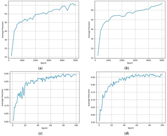
Figure 15.
Average precision curves during training for each model: (a) faster R-CNN, (b) mask R-CNN, (c) YOLOv8x, and (d) YOLOv8l-seg.
4.4. Qualitative Analysis: Object Detections in Test Images
Below are some representative cases of detections from the evaluated networks in which some detection failures can be identified.
Figure 16 presents several examples from the Faster R-CNN network. Figure 16a features multiple cacao pods, where a false positive is observed: a yellow leaf of the tree (indicative of chlorosis) is incorrectly identified as a class 4 cocoa pod (c4). Meanwhile, among the three larger reddish pods nearby, only two were accurately detected. These missed detections may be attributed to color similarity between the undetected pods and the surrounding branch or to the presence of occlusions by leaves. The model may also have undertrained on these color tones, especially if reddish pods were underrepresented in the training data. False positives like these highlight the need for more robust color diversity in the dataset.

Figure 16.
Faster R-CNN (enhanced model) detection outcomes for cacao pods under challenging field scenarios (a–d), the numbers 1 to 4 on the bbox correspond to classes c1 to c4.
Three cacao pods are visible in Figure 16b: one in the foreground (detected), one in the background (detected), and a third partially visible near the top (missed). The large pod in the foreground is confidently detected, but the third pod goes undetected, likely due to partial visibility and shadow occlusion, which affect the model’s ability to localize it. The confidence scores of the two detected pods are relatively low (~0.89–0.97), suggesting marginal certainty, possibly due to visual clutter from the forest floor.
In Figure 16c, this image presents two well-exposed pods: one red–yellow pod and one purple pod. Only the red pod is detected, while the darker pod remains undetected despite its visibility. This could stem from illumination imbalance or a bias in class confidence toward brighter, more saturated colors. The high confidence for the red pod indicates that the model can handle high-contrast instances but struggles with low-texture or less saturated objects.
Figure 16d is a complex scene with at least seven cacao pods of various colors and orientations. Only four bounding boxes are shown, meaning at least three pods are not detected. Some of the missed pods are partially occluded or facing away from the camera, introducing geometric and visual challenges. Additionally, the rotation of the image may have impacted detection robustness, suggesting that the model is sensitive to angular variance and may benefit from rotation-invariant augmentation during training.
The following Figure 17 illustrates qualitative results obtained from the Mask R-CNN model applied to cacao pods under field conditions. These samples were selected to highlight both successful detections and notable failure cases.


Figure 17.
Mask R-CNN (enhanced model) detection outcomes for cacao pods under challenging field scenarios. The variation in colors is caused by the segmentation of different instances (a–d), the numbers 1 to 4 on the bbox correspond to classes c1 to c4.
In the first image (Figure 17a), although the central pod is correctly segmented, the surrounding pods—especially those partially occluded or with color blending into the background—are entirely missed. This omission suggests the model’s limited sensitivity to subtle features under occlusion or low-contrast conditions, particularly for mature or partially hidden fruits.
The second image (Figure 17b) shows a similar trend: while the central pod is detected with high confidence, the smaller pod in the background remains undetected. The missed detection could be attributed to its relative scale, background camouflage, or insufficient representation in the training set, particularly for less prominent pod orientations.
In the third image (Figure 17c), an evident misclassification occurs. The pod on the left, which visually corresponds to class C3, was incorrectly assigned to class C4. This confusion may arise from transitional pod coloring between maturity stages, a known challenge in phenotyping where color boundaries are not always well-defined.
The fourth image (Figure 17d) presents a visually complex scene with overlapping and variably illuminated pods. Despite the cluttered background and occlusions, the model demonstrates robust performance by successfully detecting and segmenting multiple instances with high confidence. This result underscores the strength of Mask R-CNN in managing crowded environments, though minor pods remain undetected, reinforcing the need for improved recall in fine-grained detection.
These observations support the importance of dataset diversity, tailored data augmentation, and potentially class-aware or attention-enhanced architectures to handle the full spectrum of pod appearances encountered in real-world conditions.
4.5. Qualitative Evaluation: Confidence Heatmaps and Detection Performance
To further analyze the behavior of the detection model, we selected a representative set of test images and overlaid confidence heatmaps. These visualizations indicate the intensity and localization of the model’s detection confidence through colored bounding boxes.
In the first image (Figure 18a), the model successfully identifies several cocoa pods in the foreground with medium confidence (shown as green to orange). However, it fails to detect a large pod that is partially occluded in the top-left quadrant. The absence of bounding boxes or heat activation in this area suggests that the model did not pay attention to this region, likely due to visual obstructions such as branches or inadequate lighting.
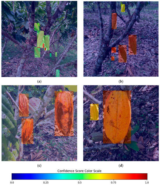
Figure 18.
Confidence-based heatmaps from Faster R-CNN (enhanced model) predictions for cacao pod detection (a–d).
In the second image (Figure 18b), while most pods are correctly detected, one detection shows a significantly low confidence score (indicated by a yellow box) and is misaligned with the ground-truth. This suggests a localization issue, potentially due to insufficient representation of that pod’s morphology or lighting conditions in the training data.
In the third image (Figure 18c), three mature cocoa pods are accurately detected with high confidence (bright orange heatmap). However, a pale pod in the background is completely overlooked, highlighting a bias in the model toward the coloration of more common pod types.
In the fourth image (Figure 18d), a single large pod is confidently detected, but smaller pods in the lower-left and upper-left regions are missed. This is likely due to variations in size, scale, or a lack of distinctive features.
These examples illustrate the following possible points:
- -
- The model performs well when pods are fully visible and well-lit.
- -
- Errors often occur when pods are partially occluded, have unusual colors, or are smaller in scale.
- -
- Confidence heatmaps provide insights into the regions the model focuses on and those it overlooks.
These findings suggest opportunities for improvement, such as the following:
- -
- Augmenting the training data with varied lighting conditions, occlusions, and less common pod appearances;
- -
- Implementing multi-scale attention mechanisms or context-based detection heads to enhance detection performance in complex backgrounds.
To further evaluate the performance of the trained Mask R-CNN X_101_32x8d_FPN_3x model, we also generated confidence heatmaps based on the predicted segmentation masks (Figure 19). These visualizations highlight the regions where the model assigns high confidence to its predictions, allowing us to qualitatively evaluate detection robustness across different classes and object scales.
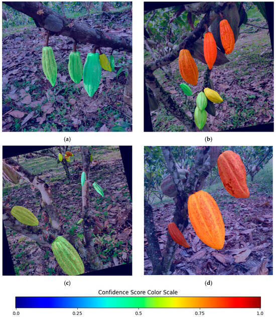
Figure 19.
Confidence-based heatmaps from Mask R-CNN (enhanced model) predictions for cacao pod detection (a–d).
In Figure 19a, this image contains multiple cacao pods in varying maturity stages. The larger pods (presumably classes c3 and c4) are detected with high confidence, as indicated by their intense red-orange overlays. However, the smaller pods located in the lower region of the image—corresponding to class c1—exhibit lower intensity in the heatmap, suggesting weak confidence scores. In some cases, these pods appear partially segmented or entirely missed by the model, highlighting the difficulty in detecting class c1 under visual occlusion and cluttered foliage.
The scene in Figure 19b presents a cluster of relatively small green pods aligned on a horizontal branch. All of them likely belong to class c2. While the model manages to localize most of the instances, the heatmap intensity is overall weaker compared to other classes, indicating lower detection confidence. Some objects appear under-segmented or merged, reinforcing the model’s limited ability to distinguish between adjacent small instances.
The image in Figure 19c contains a mix of pods of various classes and scales. Larger pods on the foreground tree trunk are well captured by the model, but again, the smaller pods at the top and on the thinner branches (likely c1) are detected with lower confidence or omitted entirely. The heatmap here reveals the spatial bias of the model—focusing more on central and prominent objects while overlooking those on the periphery.
Finally, in Figure 19d, the model successfully segments the two large pods (likely class c4 or c3) and one small pod (likely class c1) with strong confidence, as seen by the vibrant red-orange masks. In contrast, a pod on the upper left side of the tree remains undetected probably due to occlusion from the branches of the tree, suggesting a false negative for class c3. This further emphasizes the challenge of occluded pods.
5. Discussion
The findings of this study highlight the relevance and applicability of region-based convolutional neural networks (R-CNN), particularly Faster R-CNN and Mask R-CNN, for object detection and instance segmentation tasks within precision agriculture. By applying these models to the specific challenge of detecting cacao pods at different developmental stages, we explored their strengths and limitations in a real-world agricultural context, characterized by high intra-class variability, occlusions, and natural background noise.
The experimental results indicate that Mask R-CNN outperforms Faster R-CNN in terms of class-specific detection accuracy, particularly for visually complex and mature pods (class c4). This supports the hypothesis that segmentation-based approaches, which provide both bounding box detection and pixel-wise masks, are advantageous in situations where object boundaries are irregular and contextual contrast is low. The improved performance in detecting class c4 can be attributed to the model’s ability to delineate pod contours more accurately, reducing overlap confusion and enhancing spatial awareness—factors that are crucial in agriculture, where fruit counting and yield estimation depend on precise localization.
On the other hand, both Faster R-CNN and Mask R-CNN consistently faced challenges with early-stage pods (class c1), which are often smaller, less distinct from surrounding foliage, and more prone to occlusion. Despite employing selective data augmentation and class balancing strategies, this detection gap highlights the need for further improvements in feature representation—such as incorporating attention mechanisms or enhanced multi-scale feature fusion—to improve performance on smaller objects. This issue is particularly significant in agronomic monitoring, where early detection of pod development is vital for effective decision-making in disease control and harvest planning.
While YOLOv8 models were not the primary focus of this study, they were included as a benchmark to compare the performance of real-time detectors against R-CNN architectures. Interestingly, YOLOv8x and YOLOv8l-seg demonstrated superior overall mean average precision (mAP) and average precision (AP) metrics, especially in classes c3 and c4.
To further improve performance, Bayesian optimization was applied to tune key hyperparameters (learning rate and optimizer type) for both Faster R-CNN and Mask R-CNN. The search space was kept minimal to ensure feasibility, focusing on the most impactful parameters. The results showed measurable improvements in the overall mAP of both models, especially for Mask R-CNN, which benefited from the fine-tuning of learning rate and the use of SGD as the optimizer. These optimized configurations contributed to higher recall in validation subsets and better generalization to test data.
Heatmap-based confidence visualizations helped localize model uncertainty and guided the identification of failure cases. For instance, pods that were not detected often fell outside the high-confidence regions, suggesting either insufficient feature representation or suppression during the non-maximum suppression step. Error analysis of detection outputs revealed important model limitations. Several qualitative samples showed missing detections, especially of small or partially occluded pods, and occasional misclassification between similar maturity stages (e.g., c3 being confused with c4).
Ultimately, this comprehensive evaluation suggests that while Faster and Mask R-CNN architectures are valuable for their robustness and interpretability, modern models like YOLOv8x offer superior precision and inference efficiency, which are particularly advantageous for real-time deployments in agricultural environments. Nonetheless, the integration of interpretable visual diagnostics and targeted fine-tuning remains essential for adapting any architecture to the complexities of field-based crop detection.
6. Conclusions
6.1. Findings
Given the proven effectiveness of R-CNN-based architectures in handling tasks that require precise region-based reasoning, this study deliberately focused on evaluating Faster R-CNN and Mask R-CNN within the domain of precision agriculture. These models have consistently demonstrated their value in applications involving the identification of crops, fruits, and plant structures, especially in scenarios where object boundaries are irregular and visual context is complex. Their inherent ability to combine object localization with high-resolution feature extraction makes them particularly suitable for agricultural datasets like cacao pod detection, where accurate instance differentiation is critical for practical field interventions. Consequently, our analysis centers on these architectures to better understand their strengths, limitations, and potential for deployment in real-world agricultural monitoring systems.
By comparing their performance with that of cutting-edge YOLOv8 variants on a dataset of cacao pods, this research provides a benchmark using a state-of-the-art architecture for the agricultural AI community. The analysis includes class-specific performance (e.g., for pods at different maturity stages), interpretability through heatmaps and activation analysis, and model refinement via Bayesian hyperparameter optimization. This contribution is particularly relevant for researchers aiming to deploy or enhance deep learning models for tasks such as yield estimation, phenotyping, or disease detection. The findings highlight not only the strengths of R-CNN models in handling complex shapes and occlusions but also their limitations in detecting small or subtle features—guiding future work on model improvement, data augmentation, and deployment in real-world agricultural systems.
The results confirm that YOLOv8x achieves the highest performance in terms of mean average precision (mAP) and per-class accuracy, especially for well-defined, mature pods. However, the segmentation capabilities of Mask R-CNN and YOLOv8l-seg also demonstrate strong performance in visually distinct categories, supporting the value of pixel-level supervision in complex agricultural scenes.
The implementation of Bayesian optimization improved model configurations, particularly for Mask R-CNN, highlighting the importance of hyperparameter tuning in boosting model generalization.
The use of an explainability tool such as confidence heatmaps revealed detection failures, including small pod omissions and class confusions, guiding future strategies for model refinement and dataset balancing.
These findings emphasize the need for targeted improvements in the detection of early-stage pods (c1), which remain challenging due to visual ambiguity and class imbalance. Future work should explore class-specific data augmentation, attention mechanisms, and the incorporation of multispectral or depth information to enhance feature discrimination.
Overall, this research reinforces the potential of deep learning for automating phenotyping and crop monitoring in tropical agriculture, offering scalable and accurate tools for yield estimation, selective harvesting, and input optimization. The methodologies and insights presented here provide a robust foundation for deploying AI-powered detection systems in precision cocoa production and beyond.
6.2. Limitations
This study presents several limitations that should be considered when interpreting the results. First, the performance gap observed in c1 suggests that small object detection remains a significant challenge, exacerbated by occlusions, low contrast, and visual similarities with the background.
Second, all models were trained and evaluated on images acquired under similar environmental conditions and camera perspectives. This may reduce their robustness when applied to real-world scenarios involving variations in lighting, foliage density, or pod orientation. Moreover, the models were trained on 2D RGB imagery, potentially limiting their capacity to capture volumetric or textural cues relevant to pod development or damage.
A further limitation is the scope of hyperparameter optimization. While Bayesian optimization was applied to refine the learning rate and optimizer selection, other important parameters—such as batch size, feature extractor depth, or anchor settings—remained fixed due to computational constraints. Additionally, the absence of early stopping and the use of a fixed number of iterations or epochs may have led to suboptimal convergence in some cases.
One significant limitation of this study is the insufficient reporting on computational complexity, inference time, and training duration for each evaluated model. Although the analysis primarily concentrated on detection accuracy metrics like mAP, AP50, and AP75, a more thorough comparison would benefit from incorporating measures of time efficiency and resource utilization, specifically, details about runtime performance (such as frames per second, training time per epoch, and memory footprint). Future iterations of this work will incorporate a benchmarking section that includes comprehensive hardware descriptions and performance statistics to more effectively inform real-world applications.
Lastly, while performance metrics like mAP provide valuable benchmarks, they do not fully capture the agronomic value of predictions in the field. Future studies should incorporate task-specific evaluation criteria, such as correct identification per tree or per hectare, to better align with practical decision-making in precision agriculture.
6.3. Future Work
Despite the promising obtained results, several directions for future work have been identified. First, improving the detection of early-stage pods (c1) remains a critical challenge. Future studies should prioritize more aggressive class-specific data augmentation, image resolution enhancement, and attention-based feature extraction to improve discrimination of small, visually ambiguous objects.
In addition, the integration of multispectral imagery, 3D depth data, or temporal sequences from drone overflights could enrich the model’s contextual understanding and robustness under varying field conditions. Extending the annotation scheme to include occlusion levels and pod orientation could also support more nuanced detection tasks, including maturity prediction or damage assessment.
Another area of interest is the implementation of lightweight or edge-deployable versions of the best-performing models (e.g., YOLOv8-tiny) for real-time inference on embedded systems, enabling autonomous operation in the field. Finally, the development of active learning pipelines, where uncertain predictions guide future labeling efforts, would reduce annotation costs and improve model adaptability across different cocoa-growing regions.
Author Contributions
Conceptualization, J.F.R.-A. and M.J.M.-C.; methodology, J.F.R.-A. and M.J.M.-C.; software, J.F.R.-A. and M.J.M.-C.; validation, J.F.R.-A. and M.J.M.-C.; formal analysis, J.F.R.-A., M.J.M.-C., and M.F.M.-D.L.E.; investigation, J.F.R.-A., M.J.M.-C., and M.F.M.-D.L.E.; resources, J.F.R.-A. and J.W.B.-B.; data curation, M.J.M.-C.; writing—original draft preparation, J.F.R.-A.; writing—review and editing, J.W.B.-B.; visualization, M.J.M.-C.; supervision, J.F.R.-A. and J.W.B.-B.; project administration, J.F.R.-A.; funding acquisition, J.W.B.-B. All authors have read and agreed to the published version of the manuscript.
Funding
This research was funded by Universidad EAFIT, project No. 819430.
Data Availability Statement
The data presented in this study are openly available in Zenodo at https://doi.org/10.5281/zenodo.7968315 (accessed on 20 October 2024).
Acknowledgments
We want to thank the “Compañía Nacional de Chocolates” company for providing access to the farm “La Granja” in the municipality of Támesis to take the images for this work.
Conflicts of Interest
The authors declare no conflicts of interest.
References
- Fountain, A.; Hütz-Adams, F. Cocoa Barometer 2022. 2022. Available online: https://www.cocoabarometer.org (accessed on 9 February 2025).
- Cubillos-Bojacá, A.F.; García-Muñoz, M.C.; Calvo-Salamanca, A.H.; Carvajal-Rojas, G.H.; Tarazona-Diaz, M.P. Study of the physical and chemical changes during the maduration of three cocoa clones EET8, CCN51, and ICS60. J. Sci. Food Agric. 2019, 99, 5910–5917. [Google Scholar] [CrossRef] [PubMed]
- Rizzo, M.; Marcuzzo, M.; Zangari, A.; Gasparetto, A.; Albarelli, A. Fruit ripeness classification: A survey. Artif. Intell. Agric. 2023, 7, 44–57. [Google Scholar] [CrossRef]
- Nevavuori, P.; Narra, N.; Lipping, T. Crop yield prediction with deep convolutional neural networks. Comput. Electron. Agric. 2019, 163, 104859. [Google Scholar] [CrossRef]
- Apolo-Apolo, O.E.; Martínez-Guanter, J.; Egea, G.; Raja, P.; Pérez-Ruiz, M. Deep learning techniques for estimation of the yield and size of citrus fruits using a UAV. Eur. J. Agron. 2020, 115, 126030. [Google Scholar] [CrossRef]
- Bargoti, S.; Underwood, J.P. Image Segmentation for Fruit Detection and Yield Estimation in Apple Orchards. J. Field Robot. 2017, 34, 1039–1060. [Google Scholar] [CrossRef]
- Häni, N.; Roy, P.; Isler, V. A comparative study of fruit detection and counting methods for yield mapping in apple orchards. J. Field Robot. 2020, 37, 263–282. [Google Scholar] [CrossRef]
- Dorj, U.O.; Lee, M.; Yun, S.S. An yield estimation in citrus orchards via fruit detection and counting using image processing. Comput. Electron. Agric. 2017, 140, 103–112. [Google Scholar] [CrossRef]
- He, L.; Fang, W.; Zhao, G.; Wu, Z.; Fu, L.; Li, R.; Majeed, Y.; Dhupia, J. Fruit yield prediction and estimation in orchards: A state-of-the-art comprehensive review for both direct and indirect methods. Comput. Electron. Agric. 2022, 195, 106812. [Google Scholar] [CrossRef]
- Shawon, S.M.; Ema, F.B.; Mahi, A.K.; Niha, F.L.; Zubair, H.T. Crop yield prediction using machine learning: An extensive and systematic literature review. Smart Agric. Technol. 2025, 10, 100718. Available online: https://linkinghub.elsevier.com/retrieve/pii/S2772375524003228 (accessed on 1 May 2025). [CrossRef]
- Stein, M.; Bargoti, S.; Underwood, J. Image based mango fruit detection, localisation and yield estimation using multiple view geometry. Sensors 2016, 16, 1915. [Google Scholar] [CrossRef] [PubMed]
- Galindo, J.A.M.; Rosal, J.E.C.; Villaverde, J.F. Ripeness Classification of Cacao Using Cepstral-Based Statistical Features and Support Vector Machine. In Proceedings of the 2022 IEEE International Conference on Artificial Intelligence in Engineering and Technology (IICAIET), Kota Kinabalu, Malaysia, 13–15 September 2022. [Google Scholar] [CrossRef]
- Bueno, G.E.; Valenzuela, K.A.; Arboleda, E.R. Maturity classification of cacao through spectrogram and convolutional neural network. J. Teknol. dan Sist. Komput. 2020, 8, 228–233. [Google Scholar] [CrossRef]
- Gallego, A.M.; Zambrano, R.A.; Zuluaga, M.; Rodríguez, A.V.C.; Cortés, M.S.C.; Vergel, A.P.R.; Valencia, J.W.A. Analysis of fruit ripening in Theobroma cacao pod husk based on untargeted metabolomics. Phytochemistry 2022, 203, 113412. [Google Scholar] [CrossRef]
- Lockman, N.A.; Hashim, N.; Onwude, D.I. Laser-Based imaging for Cocoa Pods Maturity Detection. Food Bioprocess Tech. 2019, 12, 1928–1937. [Google Scholar] [CrossRef]
- Liu, Y.; Zheng, H.; Zhang, Y.; Zhang, Q.; Chen, H.; Xu, X.; Wang, G. ‘Is this blueberry ripe?’: A blueberry ripeness detection algorithm for use on picking robots. Front. Plant Sci. 2023, 14, 1198650. [Google Scholar] [CrossRef]
- Azodanlou, R.; Darbellay, C.; Luisier, J.L.; Villettaz, J.C.; Amadò, R. Changes in flavour and texture during the ripening of strawberries. Eur. Food Res. Technol. 2004, 218, 167–172. [Google Scholar] [CrossRef]
- Hu, C.; Liu, X.; Pan, Z.; Li, P. Automatic detection of single ripe tomato on plant combining faster R-CNN and intuitionistic fuzzy set. IEEE Access 2019, 7, 154683–154696. [Google Scholar] [CrossRef]
- Vrochidou, E.; Bazinas, C.; Manios, M.; Papakostas, G.A.; Pachidis, T.P.; Kaburlasos, V.G. Machine vision for ripeness estimation in viticulture automation. Horticulturae 2021, 7, 282. [Google Scholar] [CrossRef]
- Yang, W.; Ma, X.; An, H. Blueberry Ripeness Detection Model Based on Enhanced Detail Feature and Content-Aware Reassembly. Agronomy 2023, 13, 1613. [Google Scholar] [CrossRef]
- Mubin, N.A.; Nadarajoo, E.; Shafri, H.Z.M.; Hamedianfar, A. Young and mature oil palm tree detection and counting using convolutional neural network deep learning method. Int. J. Remote Sens. 2019, 40, 7500–7515. [Google Scholar] [CrossRef]
- Harel, B.; Parmet, Y.; Edan, Y. Maturity classification of sweet peppers using image datasets acquired in different times. Comput. Ind. 2020, 121, 103274. [Google Scholar] [CrossRef]
- Caladcad, J.A.; Cabahug, S.; Catamco, M.R.; Villaceran, P.E.; Cosgafa, L.; Cabizares, K.N.; Hermosilla, M.; Piedad, E.J. Determining Philippine coconut maturity level using machine learning algorithms based on acoustic signal. Comput. Electron. Agric. 2020, 172, 105327. [Google Scholar] [CrossRef]
- Su, F.; Zhao, Y.; Wang, G.; Liu, P.; Yan, Y. Tomato Maturity Classification Based on SE-YOLOv3-MobileNetV1 Network under Nature Greenhouse Environment. Agronomy 2022, 12, 1638. [Google Scholar] [CrossRef]
- Behera, S.K.; Rath, A.K.; Sethy, P.K. Maturity status classification of papaya fruits based on machine learning and transfer learning approach. Inf. Process. Agric. 2021, 8, 244–250. [Google Scholar] [CrossRef]
- Septiarini, A.; Sunyoto, A.; Hamdani, H.; Kasim, A.A.; Utaminingrum, F.; Hatta, H.R. Machine vision for the maturity classification of oil palm fresh fruit bunches based on color and texture features. Sci. Hortic. 2021, 286, 110245. [Google Scholar] [CrossRef]
- Restrepo-Arias, J.F.; Salinas-Agudelo, M.I.; Hernandez-Pérez, M.I.; Marulanda-Tobón, A.; Giraldo-Carvajal, M.C. RipSetCocoaCNCH12: Labeled Dataset for Ripeness Stage Detection, Semantic and Instance Segmentation of Cocoa Pods. Data 2023, 8, 112. [Google Scholar] [CrossRef]
- Chen, S.; Xiong, J.; Jiao, J.; Xie, Z.; Huo, Z.; Hu, W. Citrus fruits maturity detection in natural environments based on convolutional neural networks and visual saliency map. Precis. Agric. 2022, 23, 1515–1531. [Google Scholar] [CrossRef]
- Bazame, H.C.; Molin, J.P.; Althoff, D.; Martello, M. Detection, classification, and mapping of coffee fruits during harvest with computer vision. Comput. Electron. Agric. 2021, 183, 106066. [Google Scholar] [CrossRef]
- Arendse, E.; Fawole, O.A.; Magwaza, L.S.; Opara, U.L. Non-destructive prediction of internal and external quality attributes of fruit with thick rind: A review. J. Food Eng. 2018, 217, 11–23. [Google Scholar] [CrossRef]
- Wang, H.; Zhang, G.; Cao, H.; Hu, K.; Wang, Q.; Deng, Y.; Gao, J.; Tang, Y. Geometry-Aware 3D Point Cloud Learning for Precise Cutting-Point Detection in Unstructured Field Environments. J. Field Robotics 2025. [Google Scholar] [CrossRef]
- Wu, F.; Zhu, R.; Meng, F.; Qiu, J.; Yang, X.; Li, J.; Zou, X. An Enhanced Cycle Generative Adversarial Network Approach for Nighttime Pineapple Detection of Automated Harvesting Robots. Agronomy 2024, 14, 3002. [Google Scholar] [CrossRef]
- Ali, M.M.; Hashim, N.; Shahamshah, M.I. Durian (Durio zibethinus) ripeness detection using thermal imaging with multivariate analysis. Postharvest Biol. Technol. 2021, 176, 111517. [Google Scholar] [CrossRef]
- Begum, N.; Hazarika, M.K. Maturity detection of tomatoes using transfer learning. Meas. Food 2022, 7, 100038. [Google Scholar] [CrossRef]
- Khojastehnazhand, M.; Mohammadi, V.; Minaei, S. Maturity detection and volume estimation of apricot using image processing technique. Sci. Hortic. 2019, 251, 247–251. [Google Scholar] [CrossRef]
- Sahu, D.; Potdar, R.M. Defect Identification and Maturity Detection of Mango Fruits Using Image Analysis. Artic. Int. J. Artif. Intell. 2017, 1, 5–14. Available online: http://www.sciencepublishinggroup.com/j/ajai (accessed on 2 May 2025). [CrossRef]
- Saranya, N.; Srinivasan, K.; Kumar, S.K.P. Banana ripeness stage identification: A deep learning approach. J. Ambient. Intell. Humaniz. Comput. 2022, 13, 4033–4039. [Google Scholar] [CrossRef]
- Wan, P.; Toudeshki, A.; Tan, H.; Ehsani, R. A methodology for fresh tomato maturity detection using computer vision. Comput. Electron. Agric. 2018, 146, 43–50. [Google Scholar] [CrossRef]
- Xiao, B.; Nguyen, M.; Yan, W.Q. Fruit ripeness identification using YOLOv8 model. Multimed. Tools Appl. 2024, 83, 28039–28056. [Google Scholar] [CrossRef]
- Gai, R.L.; Wei, K.; Wang, P.F. SSMDA: Self-Supervised Cherry Maturity Detection Algorithm Based on Multi-Feature Contrastive Learning. Agriculture 2023, 13, 939. [Google Scholar] [CrossRef]
- Han, W.; Hao, W.; Sun, J.; Xue, Y.; Li, W. Tomatoes Maturity Detection Approach Based on YOLOv5 and Attention Mechanisms. In Proceedings of the 2022 IEEE 4th International Conference on Civil Aviation Safety and Information Technology (ICCASIT), Dali, China, 12–14 October 2022; pp. 1363–1371. [Google Scholar] [CrossRef]
- Tao, Z.; Li, K.; Rao, Y.; Li, W.; Zhu, J. Strawberry Maturity Recognition Based on Improved YOLOv5. Agronomy 2024, 14, 460. [Google Scholar] [CrossRef]
- Jiang, S.; Liu, Z.; Hua, J.; Zhang, Z.; Zhao, S.; Xie, F.; Ao, J.; Wei, Y.; Lu, J.; Li, Z.; et al. A Real-Time Detection and Maturity Classification Method for Loofah. Agronomy 2023, 13, 2144. [Google Scholar] [CrossRef]
- Zhu, X.; Chen, F.; Zhang, X.; Zheng, Y.; Peng, X.; Chen, C. Detection the maturity of multi-cultivar olive fruit in orchard environments based on Olive-EfficientDet. Sci. Hortic. 2024, 324, 112607. [Google Scholar] [CrossRef]
- Wang, C.; Wang, C.; Wang, L.; Wang, J.; Liao, J.; Li, Y.; Lan, Y. A Lightweight Cherry Tomato Maturity Real-Time Detection Algorithm Based on Improved YOLOV5n. Agronomy 2023, 13, 2106. [Google Scholar] [CrossRef]
- Wang, Z.; Ling, Y.; Wang, X.; Meng, D.; Nie, L.; An, G.; Wang, X. An improved Faster R-CNN model for multi-object tomato maturity detection in complex scenarios. Ecol. Inform. 2022, 72, 101886. [Google Scholar] [CrossRef]
- Xu, D.; Zhao, H.; Lawal, O.M.; Lu, X.; Ren, R.; Zhang, S. An Automatic Jujube Fruit Detection and Ripeness Inspection Method in the Natural Environment. Agronomy 2023, 13, 451. [Google Scholar] [CrossRef]
- Zhang, M.; Shen, M.; Pu, Y.; Li, H.; Zhang, B.; Zhang, Z.; Ren, X.; Zhao, J. Rapid Identification of Apple Maturity Based on Multispectral Sensor Combined with Spectral Shape Features. Horticulturae 2022, 8, 361. [Google Scholar] [CrossRef]
- Redmon, J.; Divvala, S.; Girshick, R.; Farhadi, A. You Only Look Once: Unified, Real-Time Object Detection. 2015. Available online: http://arxiv.org/abs/1506.02640 (accessed on 5 May 2025).
- Bochkovskiy, A.; Wang, C.-Y.; Liao, H.-Y.M. YOLOv4: Optimal Speed and Accuracy of Object Detection. 2020. Available online: http://arxiv.org/abs/2004.10934 (accessed on 5 May 2025).
- Wang, C.-Y.; Bochkovskiy, A.; Liao, H.-Y.M. YOLOv7: Trainable Bag-of-Freebies Sets New State-of-the-Art for Real-Time Object Detectors. 2022. Available online: http://arxiv.org/abs/2207.02696 (accessed on 5 May 2025).
- Redmon, J.; YOLO, A.F. 9000: Better, Faster, Stronger. Available online: http://arxiv.org/abs/1612.08242 (accessed on 5 May 2025).
- Redmon, J. YOLOv3: An Incremental Improvement. 2018. Available online: http://arxiv.org/abs/1804.02767 (accessed on 5 May 2025).
- Li, C.; Li, L.; Jiang, H.; Weng, K.; Geng, Y.; Li, L.; Ke, Z.; Li, Q.; Cheng, M.; Nie, W.; et al. YOLOv6: A Single-Stage Object Detection Framework for Industrial Applications. 2022. Available online: http://arxiv.org/abs/2209.02976 (accessed on 5 May 2025).
- Tang, Y.; Zhou, H.; Wang, H.; Zhang, Y. Fruit detection and positioning technology for a Camellia oleifera C. Abel orchard based on improved YOLOv4-tiny model and binocular stereo vision. Expert Syst. Appl. 2023, 211, 118573. [Google Scholar] [CrossRef]
- Li, P.; Zheng, J.; Li, P.; Long, H.; Li, M.; Gao, L. Tomato Maturity Detection and Counting Model Based on MHSA-YOLOv8. Sensors 2023, 23, 6701. [Google Scholar] [CrossRef] [PubMed]
- Sapkota, R.; Ahmed, D.; Karkee, M. Comparing YOLOv8 and Mask R-CNN for instance segmentation in complex orchard environments. Artif. Intell. Agric. 2024, 13, 84–99. [Google Scholar] [CrossRef]
- Liu, T.H.; Nie, X.-N.; Wu, J.-M.; Zhang, D.; Liu, W.; Cheng, Y.-F.; Zheng, Y.; Qiu, J.; Qi, L. Pineapple (Ananas comosus) fruit detection and localization in natural environment based on binocular stereo vision and improved YOLOv3 model. Precis. Agric. 2023, 24, 139–160. [Google Scholar] [CrossRef]
- Ren, S.; He, K.; Girshick, R.; Sun, J. Faster R-CNN: Towards Real-Time Object Detection with Region Proposal Networks. IEEE Trans. Pattern Anal. Mach. Intell. 2017, 39, 1137–1149. Available online: http://arxiv.org/abs/1506.01497 (accessed on 1 March 2025). [CrossRef] [PubMed]
- He, K.; Gkioxari, G.; Dollár, P. Mask R-CNN. arXiv 2018, arXiv:1703.06870. [Google Scholar]
- Huang, F.; Li, Y.; Liu, Z.; Gong, L.; Liu, C. A Method for Calculating the Leaf Area of Pak Choi Based on an Improved Mask R-CNN. Agriculture 2024, 14, 101. [Google Scholar] [CrossRef]
- Gong, X.; Zhang, S. A High-Precision Detection Method of Apple Leaf Diseases Using Improved Faster R-CNN. Agriculture 2023, 13, 240. [Google Scholar] [CrossRef]
- Li, Y.; Wang, Y.; Xu, D.; Zhang, J.; Wen, J. An Improved Mask RCNN Model for Segmentation of ‘Kyoho’ (Vitis labruscana) Grape Bunch and Detection of Its Maturity Level. Agriculture 2023, 13, 914. [Google Scholar] [CrossRef]
- Jia, W.; Wei, J.; Zhang, Q.; Pan, N.; Niu, Y.; Yin, X.; Ding, Y.; Ge, X. Accurate segmentation of green fruit based on optimized mask RCNN application in complex orchard. Front. Plant Sci. 2022, 13, 955256. [Google Scholar] [CrossRef] [PubMed]
- Huang, Y.P.; Wang, T.H.; Basanta, H. Using Fuzzy Mask R-CNN Model to Automatically Identify Tomato Ripeness. IEEE Access 2020, 8, 207672–207682. [Google Scholar] [CrossRef]
- Tu, S.; Xue, Y.; Zheng, C.; Qi, Y.; Wan, H.; Mao, L. Detection of passion fruits and maturity classification using Red-Green-Blue Depth images. Biosyst. Eng. 2018, 175, 156–167. [Google Scholar] [CrossRef]
- Tu, S.; Pang, J.; Liu, H.; Zhuang, N.; Chen, Y.; Zheng, C.; Wan, H.; Xue, Y. Passion fruit detection and counting based on multiple scale faster R-CNN using RGB-D images. Precis. Agric. 2020, 21, 1072–1091. [Google Scholar] [CrossRef]
- Zhao, Z.; Hicks, Y.; Sun, X.; Luo, C. Peach ripeness classification based on a new one-stage instance segmentation model. Comput. Electron. Agric. 2023, 214, 108369. [Google Scholar] [CrossRef]
- Li, J.; Zhu, Z.; Liu, H.; Su, Y.; Deng, L. Strawberry R-CNN: Recognition and counting model of strawberry based on improved faster R-CNN. Ecol. Inform. 2023, 77, 102210. [Google Scholar] [CrossRef]
- Deka, B.; Chakraborty, D. UAV Sensing-Based Litchi Segmentation Using Modified Mask-RCNN for Precision Agriculture. IEEE Trans. AgriFood Electron. 2024, 2, 509–517. [Google Scholar] [CrossRef]
- Guo, Z.; Shi, Y.; Ahmad, I. Design of smart citrus picking model based on Mask RCNN and adaptive threshold segmentation. PeerJ Comput. Sci. 2024, 10, e1865. [Google Scholar] [CrossRef] [PubMed]
- Siricharoen, P.; Yomsatieankul, W.; Bunsri, T. Fruit maturity grading framework for small dataset using single image multi-object sampling and Mask R-CNN. Smart Agric. Technol. 2023, 3, 100130. [Google Scholar] [CrossRef]
- Jiao, L.; Dong, S.; Zhang, S.; Xie, C.; Wang, H. AF-RCNN: An anchor-free convolutional neural network for multi-categories agricultural pest detection. Comput. Electron. Agric. 2020, 174, 105522. [Google Scholar] [CrossRef]
- Sharma, A.; Kumar, V.; Longchamps, L. Comparative performance of YOLOv8, YOLOv9, YOLOv10, YOLOv11 and Faster R-CNN models for detection of multiple weed species. Smart Agric. Technol. 2024, 9, 100648. [Google Scholar] [CrossRef]
- Maru, R.; Kamat, A.; Shah, M.; Kute, P.; Shrawne, S.C.; Sambhe, V. Improved Faster RCNN for Ripeness and Size Estimation of Mangoes with multi-label output. In Proceedings of the 2024 International Conference on Computational Intelligence and Network Systems (CINS), Dubai, United Arab Emirates, 28–29 November 2024. [Google Scholar] [CrossRef]
- Girshick, R.; Donahue, J.; Darrell, T.; Malik, J. Rich Feature Hierarchies for Accurate Object Detection and Semantic Segmentation. 2014. Available online: http://arxiv.org/abs/1311.2524 (accessed on 5 March 2025).
- Ayikpa, K.J.; Mamadou, D.; Gouton, P.; Adou, K.J. Classification of Cocoa Pod Maturity Using Similarity Tools on an Image Database: Comparison of Feature Extractors and Color Spaces. Data 2023, 8, 99. [Google Scholar] [CrossRef]
- Veites-Campos, S.A.; Ramírez-Betancour, R.; González-Pérez, M. Identification of Cocoa Pods with Image Processing and Artificial Neural Networks. Int. J. Adv. Eng. Manag. Sci. 2018, 4, 510–518. [Google Scholar] [CrossRef]
- Heredia-Gómez, J.F.; Rueda-Gómez, J.P.; Talero-Sarmiento, L.H.; Ramírez-Acuña, J.S.; Coronado-Silva, R.A. Cocoa pods ripeness estimation, using convolutional neural networks in an embedded system. Rev. Colomb. de Comput. 2020, 21, 42–55. [Google Scholar] [CrossRef]
- Baculio, N.G.; Barbosa, J.B. An Objective Classification Approach of Cacao Pods using Local Binary Pattern Features and Artificial Neural Network Architecture (ANN). Indian J. Sci. Technol. 2022, 15, 495–504. [Google Scholar] [CrossRef]
- Kim, E.C.; Hong, S.-J.; Kim, S.-Y.; Lee, C.-H.; Kim, S.; Kim, H.-J.; Kim, G. CNN-based object detection and growth estimation of plum fruit (Prunus mume) using RGB and depth imaging techniques. Sci. Rep. 2022, 12, 20796. [Google Scholar] [CrossRef]
- Wu, T.; Miao, Z.; Huang, W.; Han, W.; Guo, Z.; Li, T. SGW-YOLOv8n: An Improved YOLOv8n-Based Model for Apple Detection and Segmentation in Complex Orchard Environments. Agriculture 2024, 14, 1958. [Google Scholar] [CrossRef]
- Xiao, F.; Wang, H.; Xu, Y.; Zhang, R. Fruit Detection and Recognition Based on Deep Learning for Automatic Harvesting: An Overview and Review. Agronomy 2023, 13, 1625. [Google Scholar] [CrossRef]
- Girshick, R. Fast R-CNN. In Proceedings of the 2015 IEEE International Conference on Computer Vision (ICCV), Santiago, Chile, 7–13 December 2015; pp. 1440–1448. [Google Scholar] [CrossRef]
- Zhao, X.; Li, W.; Zhang, Y.; Gulliver, T.A.; Chang, S.; Feng, Z. A Faster RCNN-based Pedestrian Detection System. In Proceedings of the 2016 IEEE 84th Vehicular Technology Conference (VTC-Fall), Montreal, QC, Canada, 18–21 September 2016. [Google Scholar]
- Cheng, B.; Wei, Y.; Shi, H.; Feris, R.; Xiong, J.; Huang, T. Revisiting RCNN: On Awakening the Classification Power of Faster RCNN. In Proceedings of the Computer Vision—ECCV 2018, Munich, Germany, 8–14 September 2018. [Google Scholar]
- Roh, M.-C.; Lee, J. Refining Faster-RCNN for Accurate Object Detection. In Proceedings of the 2017 Fifteenth IAPR International Conference on Machine Vision Applications (MVA), Nagoya, Japan, 8–12 May 2017. [Google Scholar]
- He, K.; Gkioxari, G.; Dollár, P.; Girshick, R. Mask R-CNN. IEEE Trans. Pattern Anal. Mach. Intell. 2020, 42, 386–397. [Google Scholar] [CrossRef] [PubMed]
- Ahmed, B.; Gulliver, T.A.; Alzahir, S. Image splicing detection using mask-RCNN. Signal Image Video Process 2020, 14, 1035–1042. [Google Scholar] [CrossRef]
- Nowozin, S. Optimal decisions from probabilistic models: The intersection-over-union case. In Proceedings of the IEEE Computer Society Conference on Computer Vision and Pattern Recognition, Columbus, OH, USA, 24–27 June 2014; pp. 548–555. [Google Scholar] [CrossRef]
- Lin, T.-Y.; Maire, M.; Belongie, S.; Hays, J.; Perona, P.; Ramanan, D.; Dollár, P.; Zitnick, C.L. Microsoft COCO: Common Objects in Context. In Proceedings of the Computer Vision–ECCV 2014: 13th European Conference, Zurich, Switzerland, 6–12 September 2014. [Google Scholar] [CrossRef]
- Wu, J.; Chen, X.Y.; Zhang, H.; Xiong, L.D.; Lei, H.; Deng, S.H. Hyperparameter optimization for machine learning models based on Bayesian optimization. J. Electron. Sci. Technol. 2019, 17, 26–40. [Google Scholar] [CrossRef]
- Alibrahim, H.; Ludwig, S.A. Hyperparameter Optimization: Comparing Genetic Algorithm against Grid Search and Bayesian Optimization. In Proceedings of the 2021 IEEE Congress on Evolutionary Computation (CEC), Kraków, Poland, 28 June–1 July 2021; pp. 1551–1559. [Google Scholar] [CrossRef]
- Zhou, B.; Khosla, A.; Lapedriza, A.; Oliva, A.; Torralba, A. Learning Deep Features for Discriminative Localization. 2016. Available online: http://cnnlocalization.csail.mit.edu (accessed on 10 June 2025).
- Selvaraju, R.R.; Cogswell, M.; Das, A.; Vedantam, R.; Parikh, D.; Batra, D. Grad-CAM: Visual Explanations from Deep Networks via Gradient-based Localization. 2017. Available online: http://gradcam.cloudcv.org (accessed on 10 June 2025).

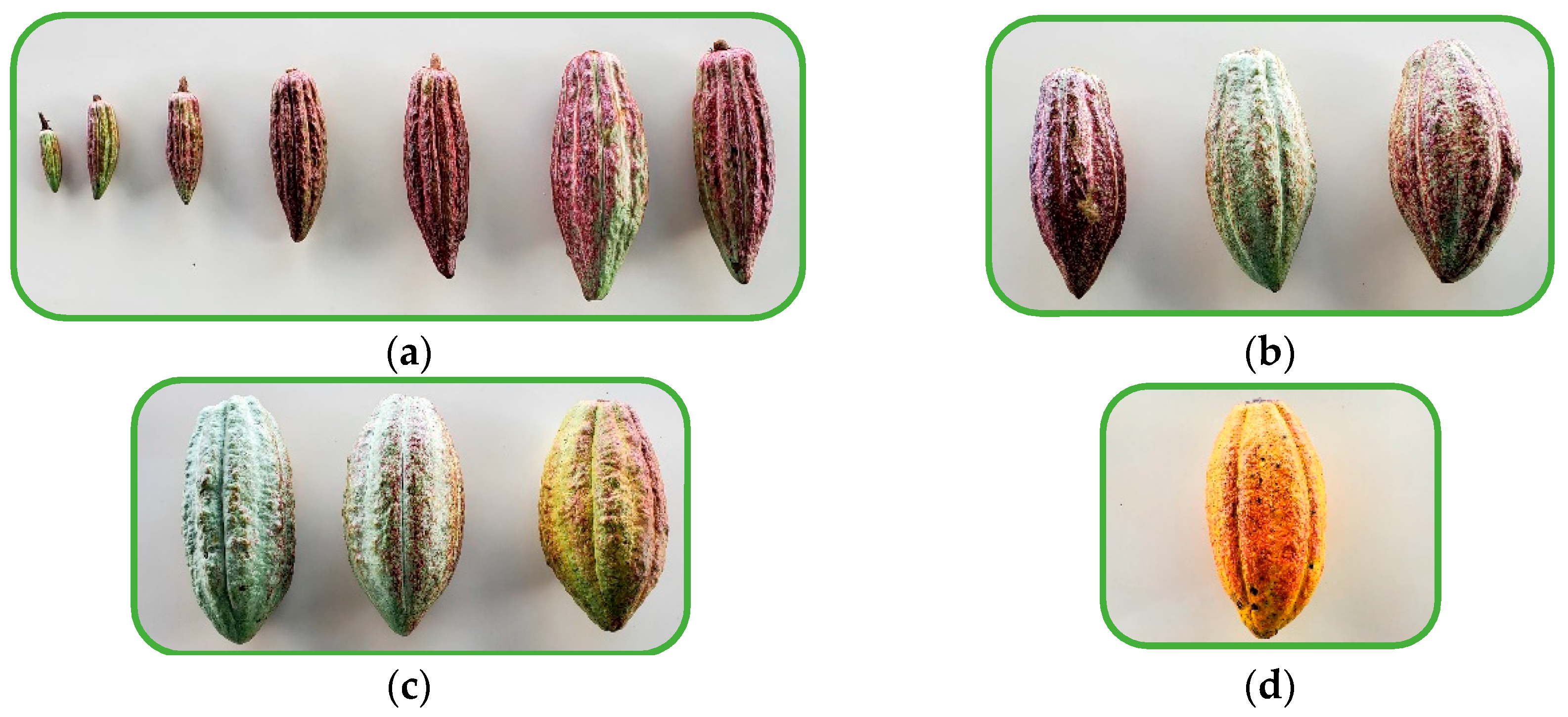
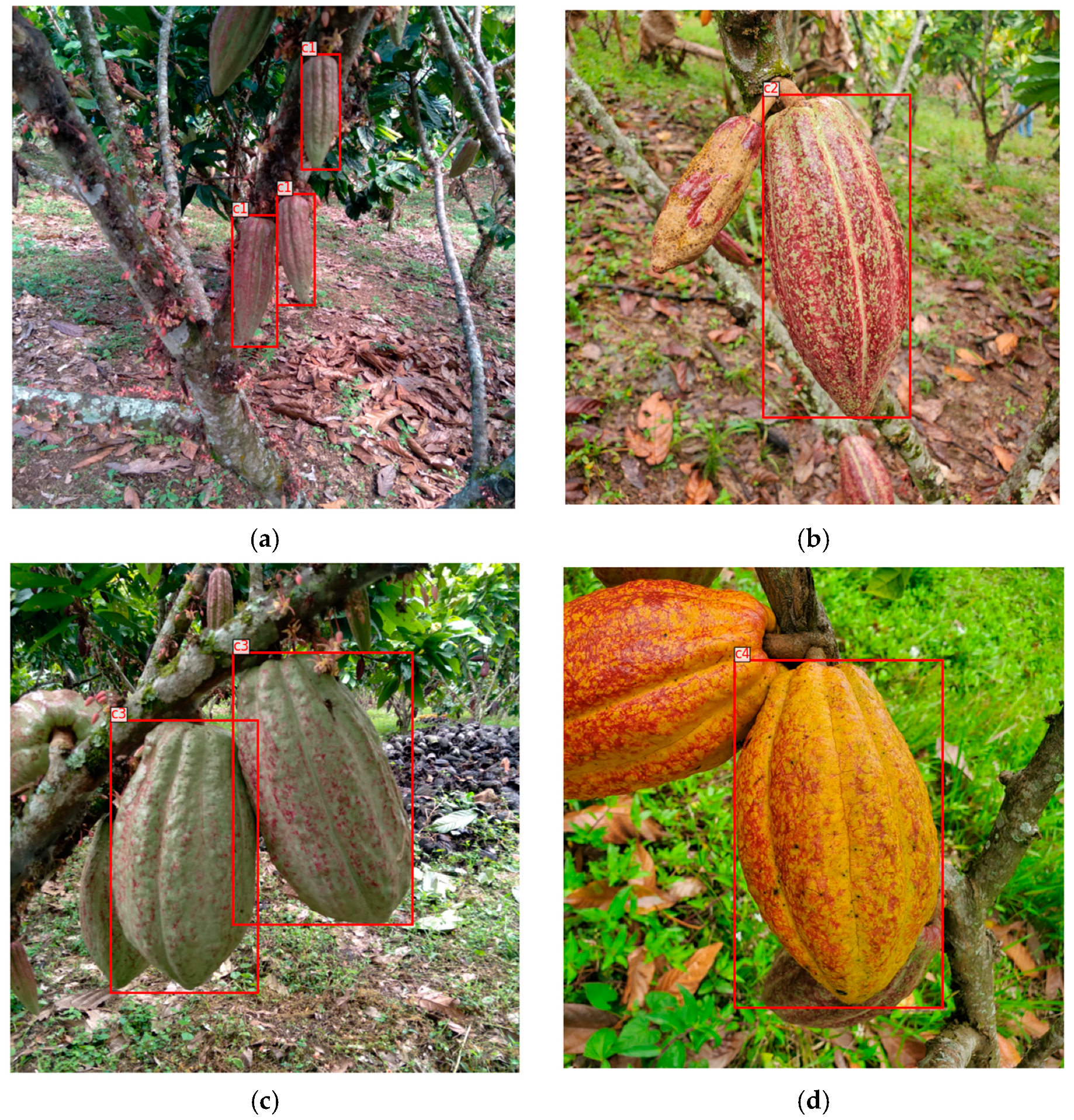
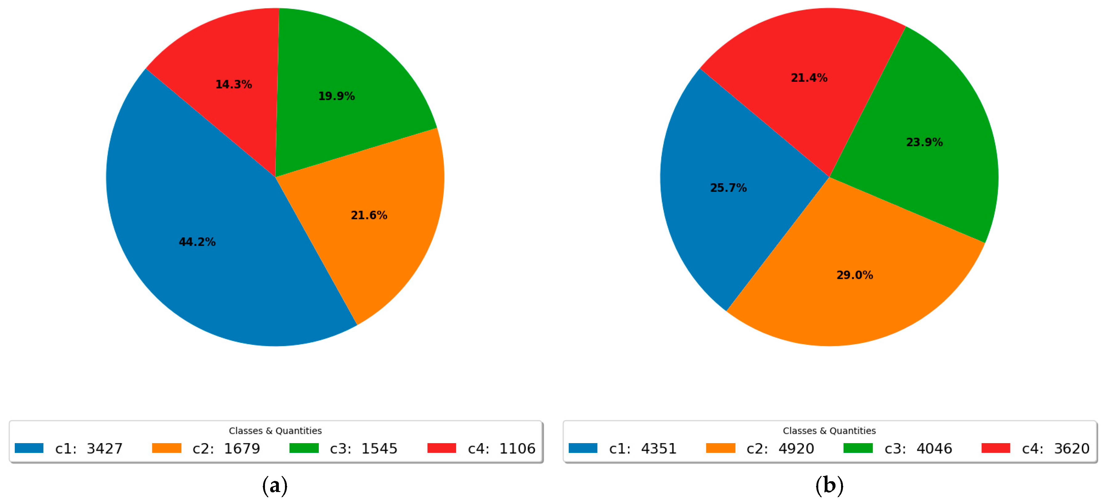
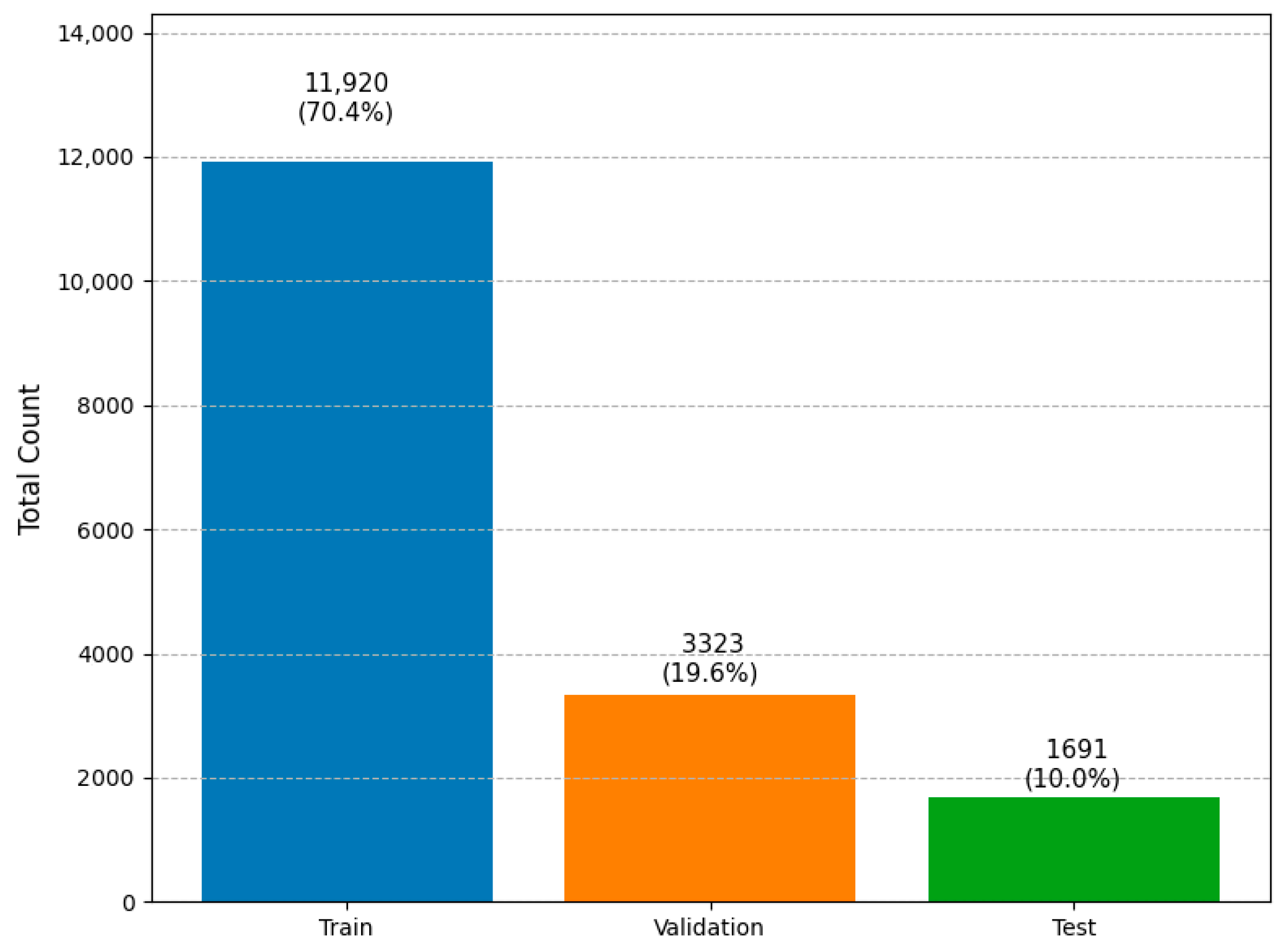

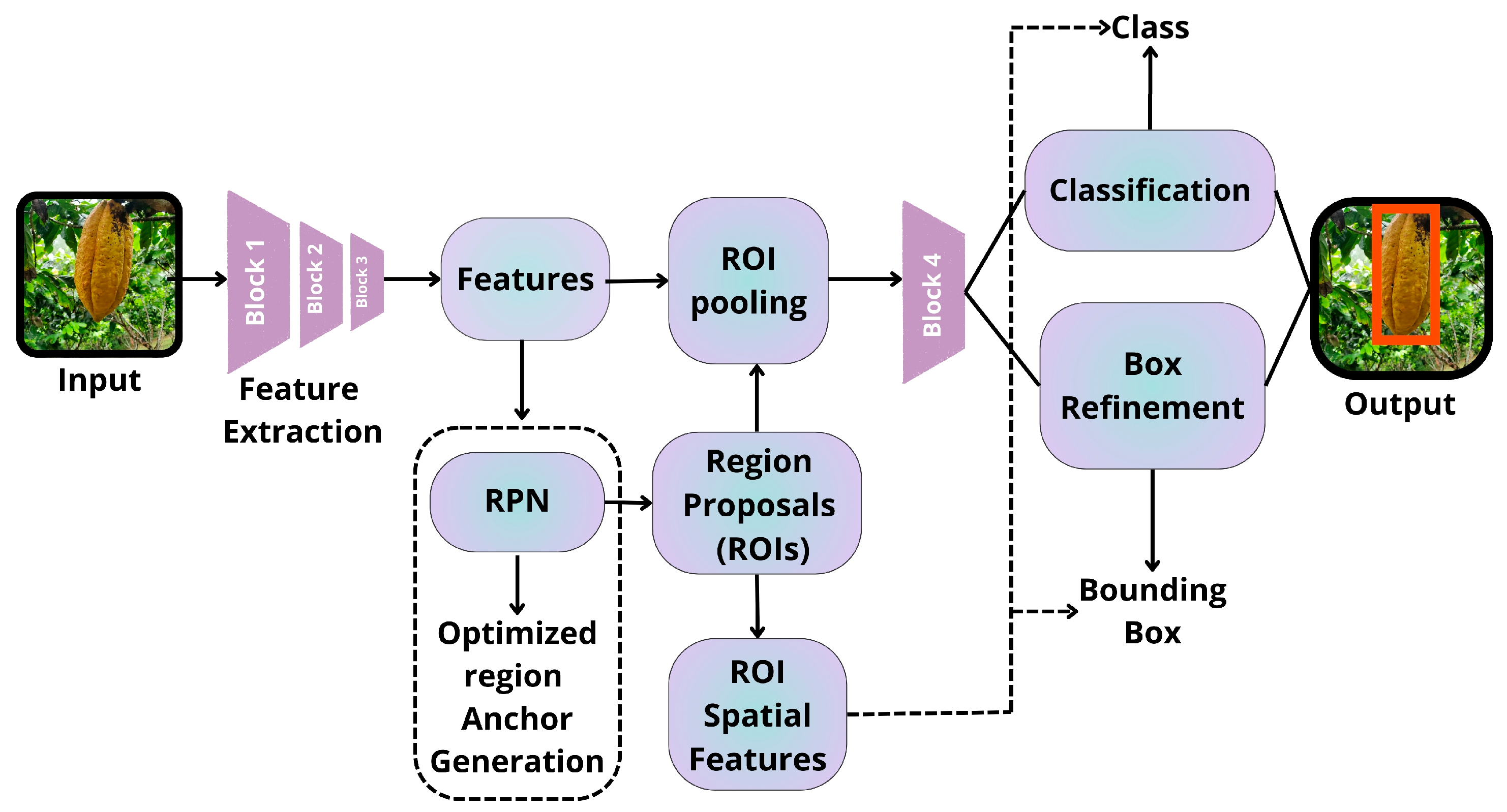
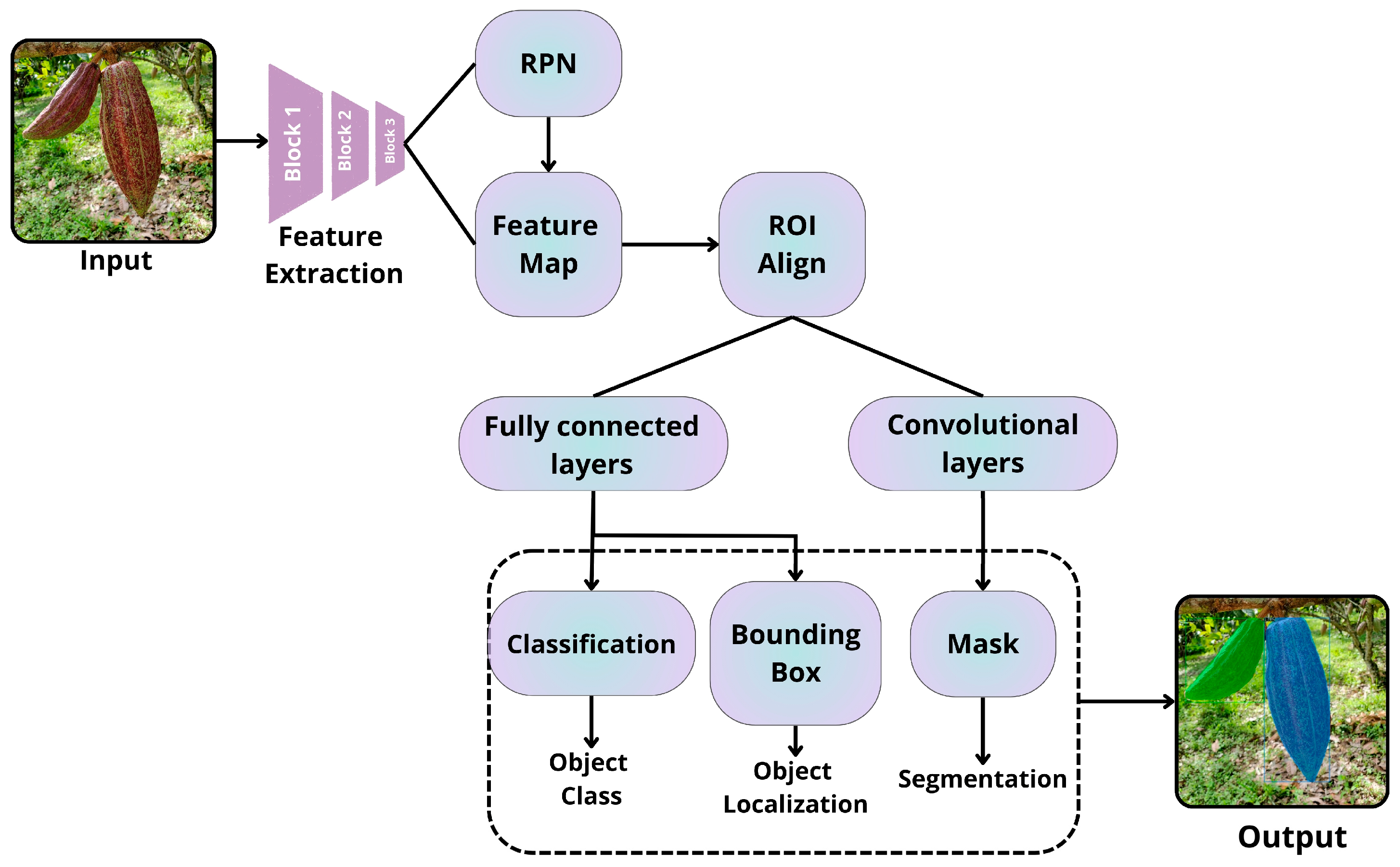

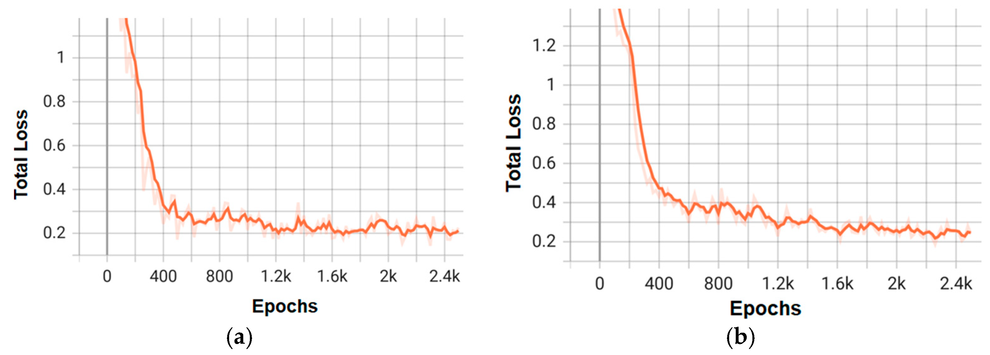
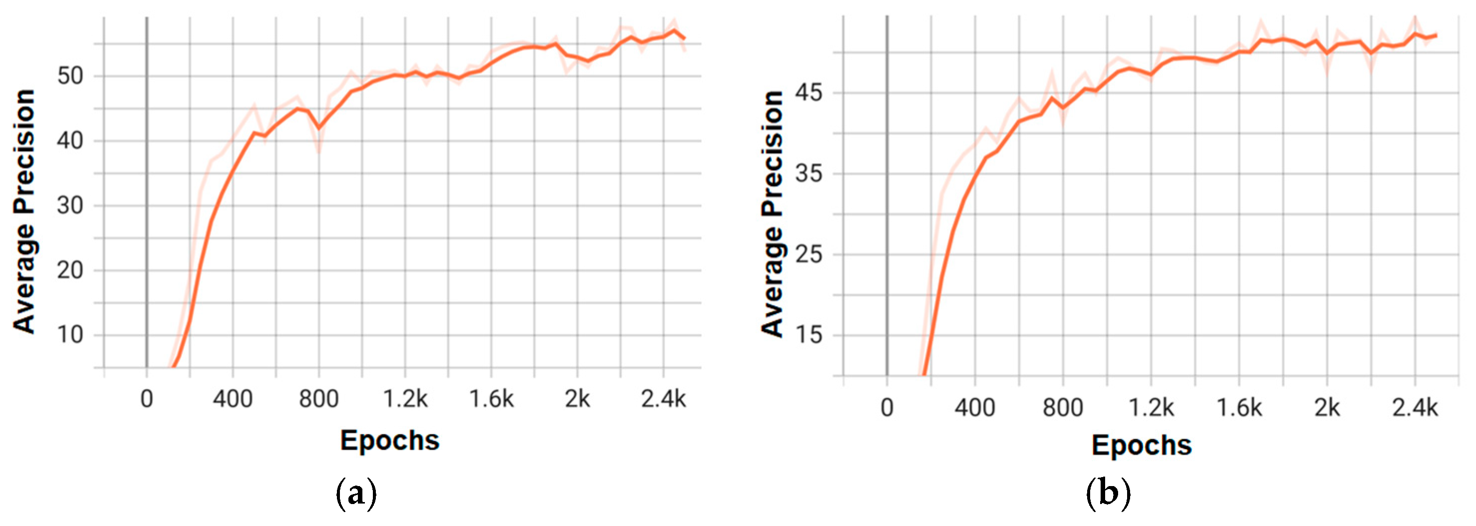
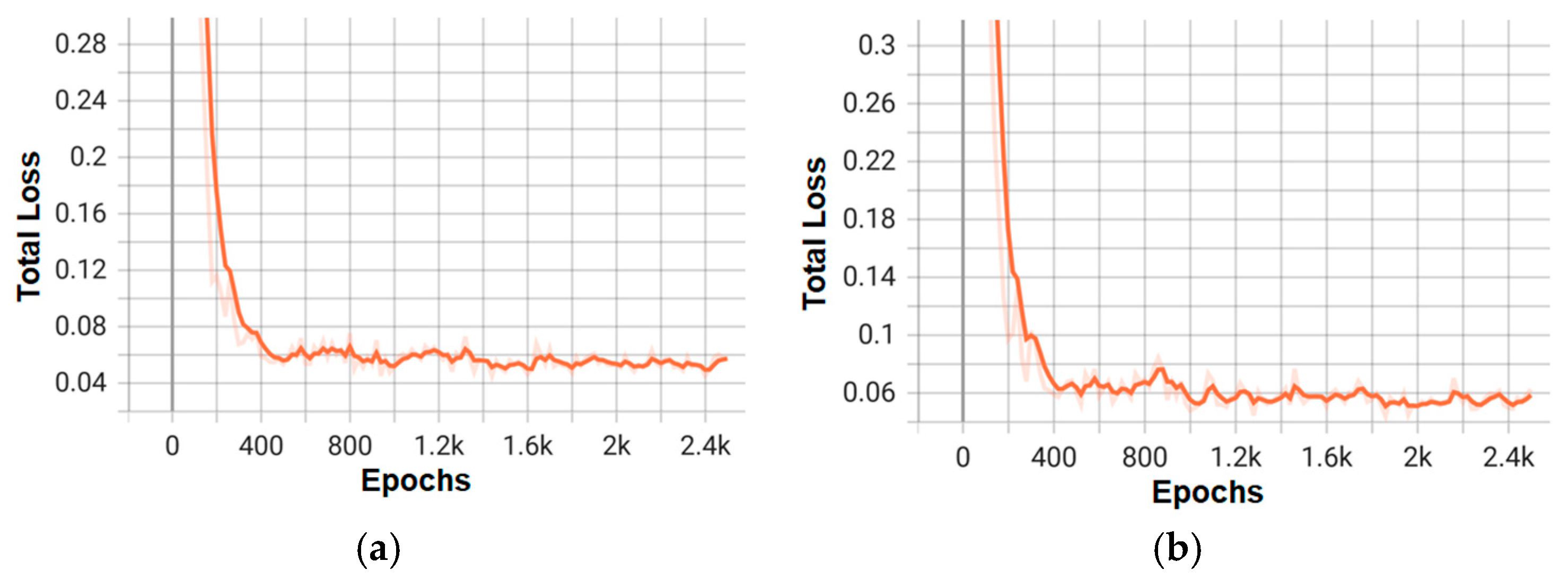
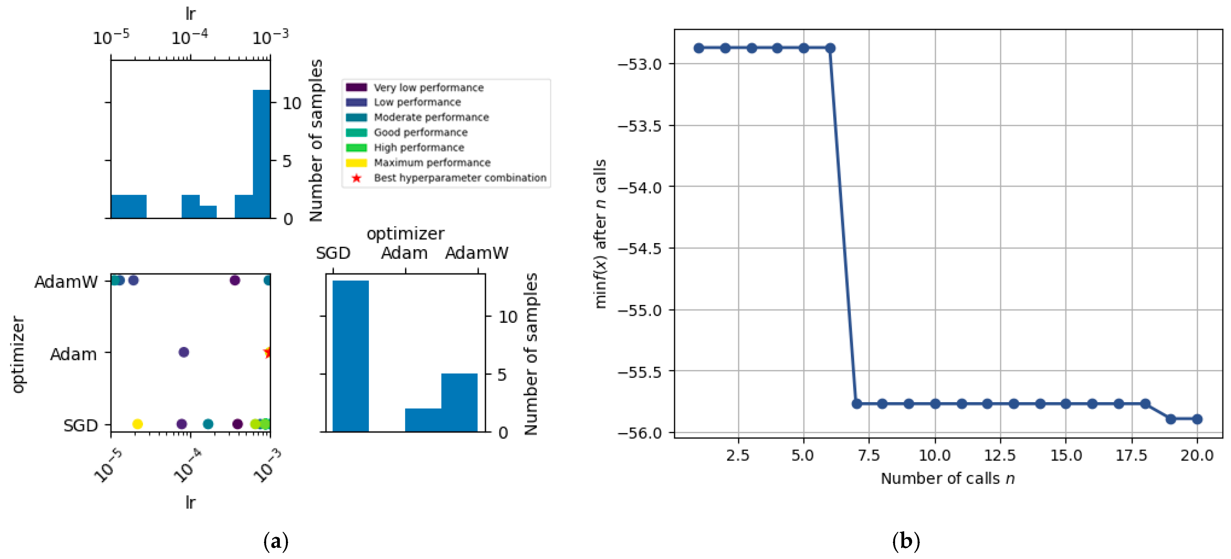
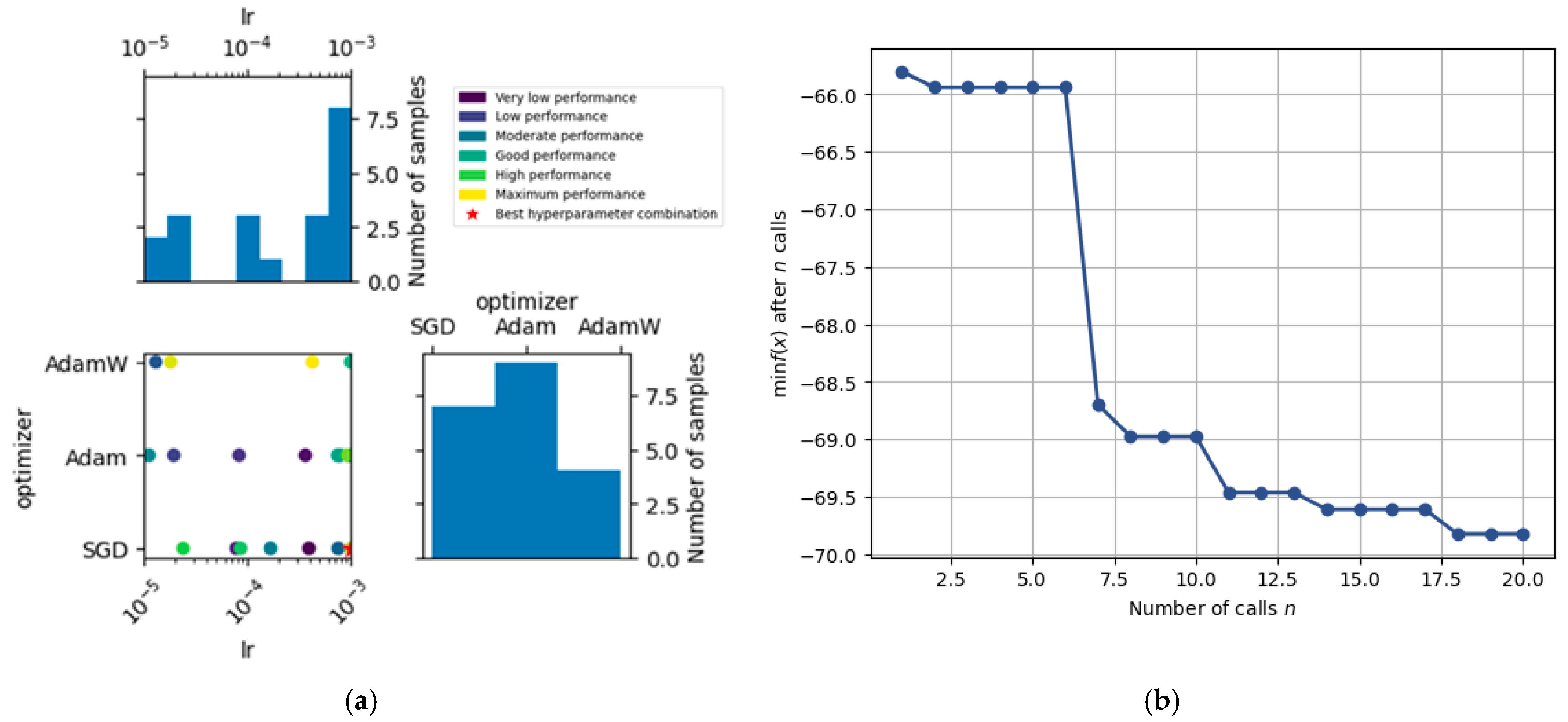
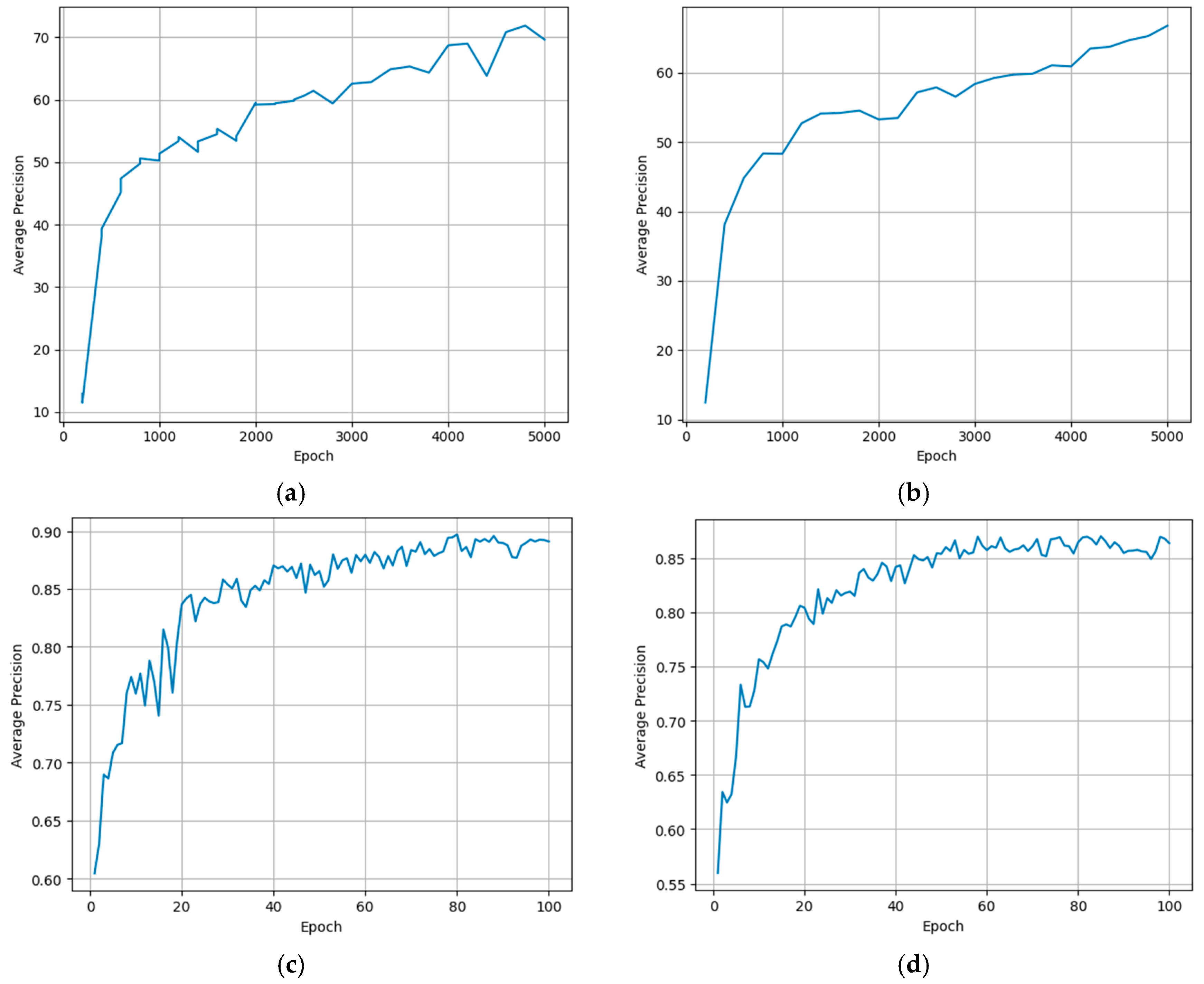
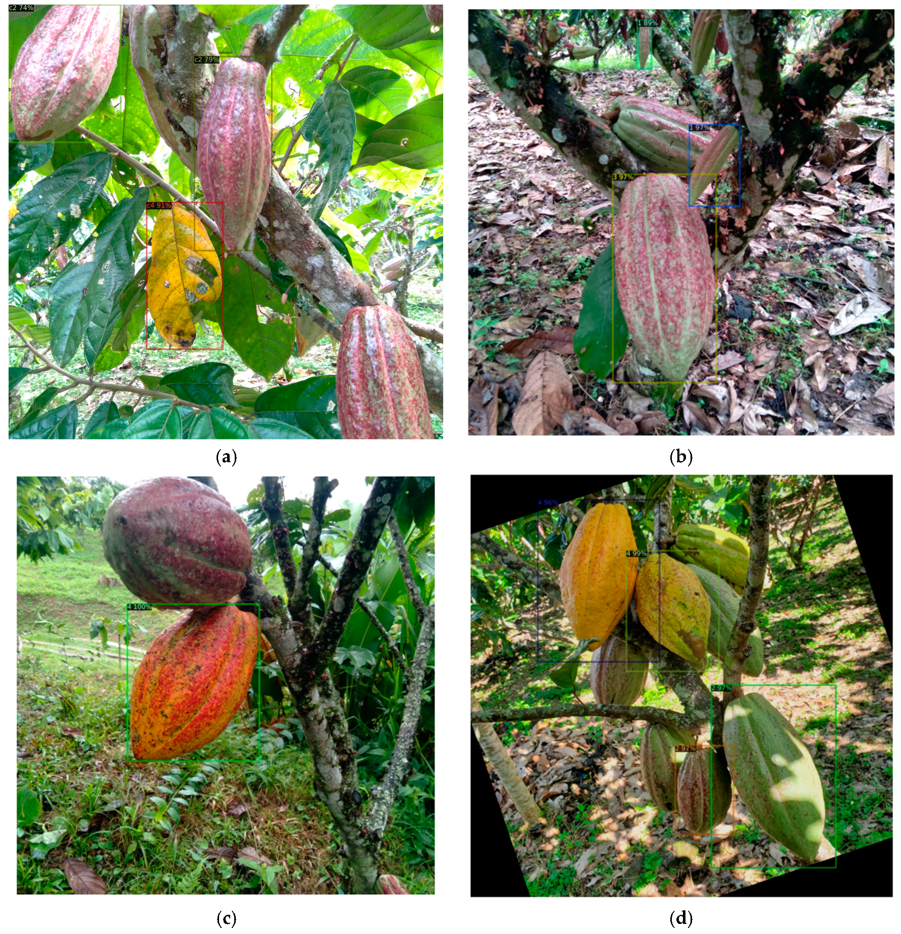
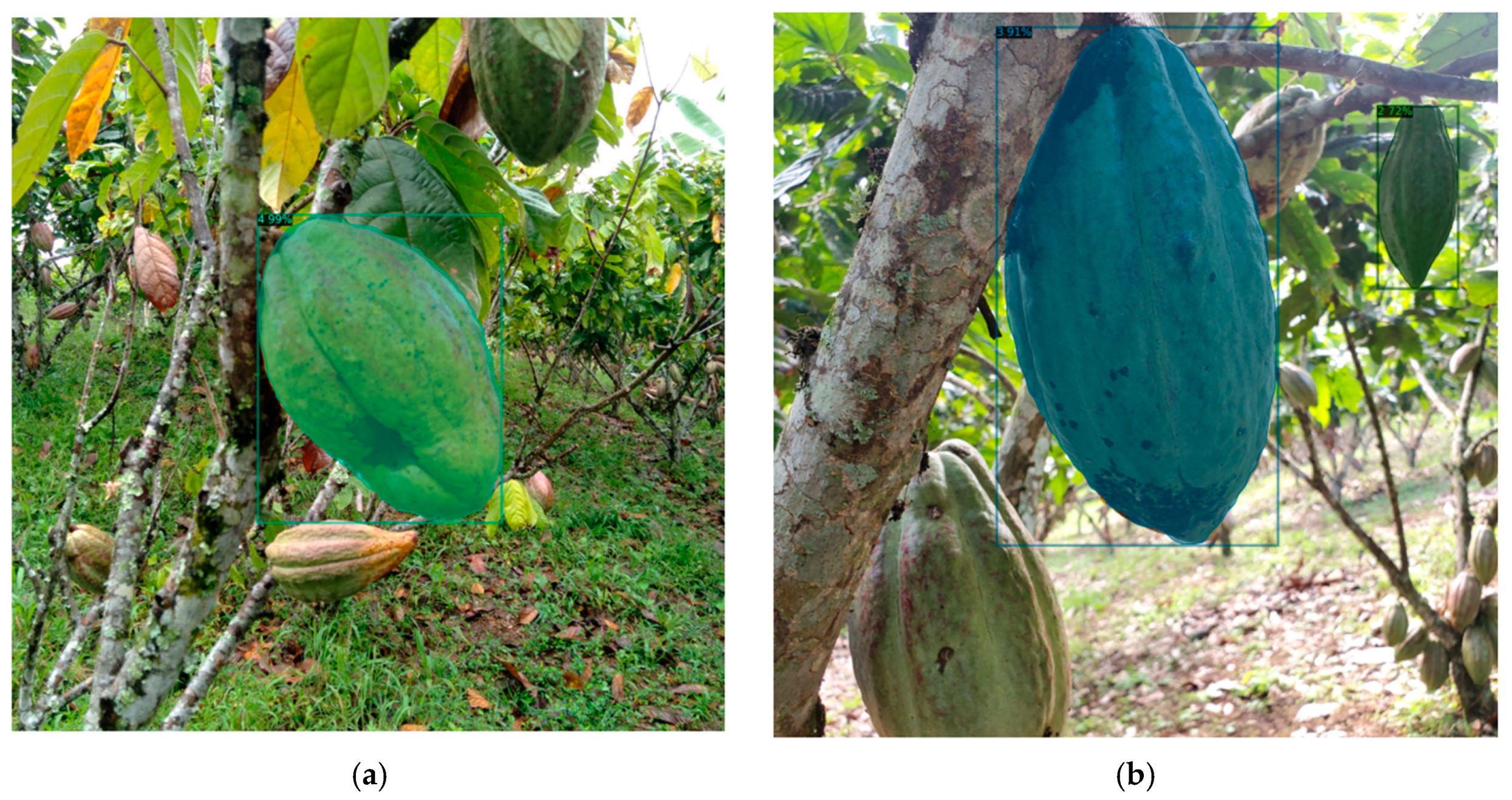
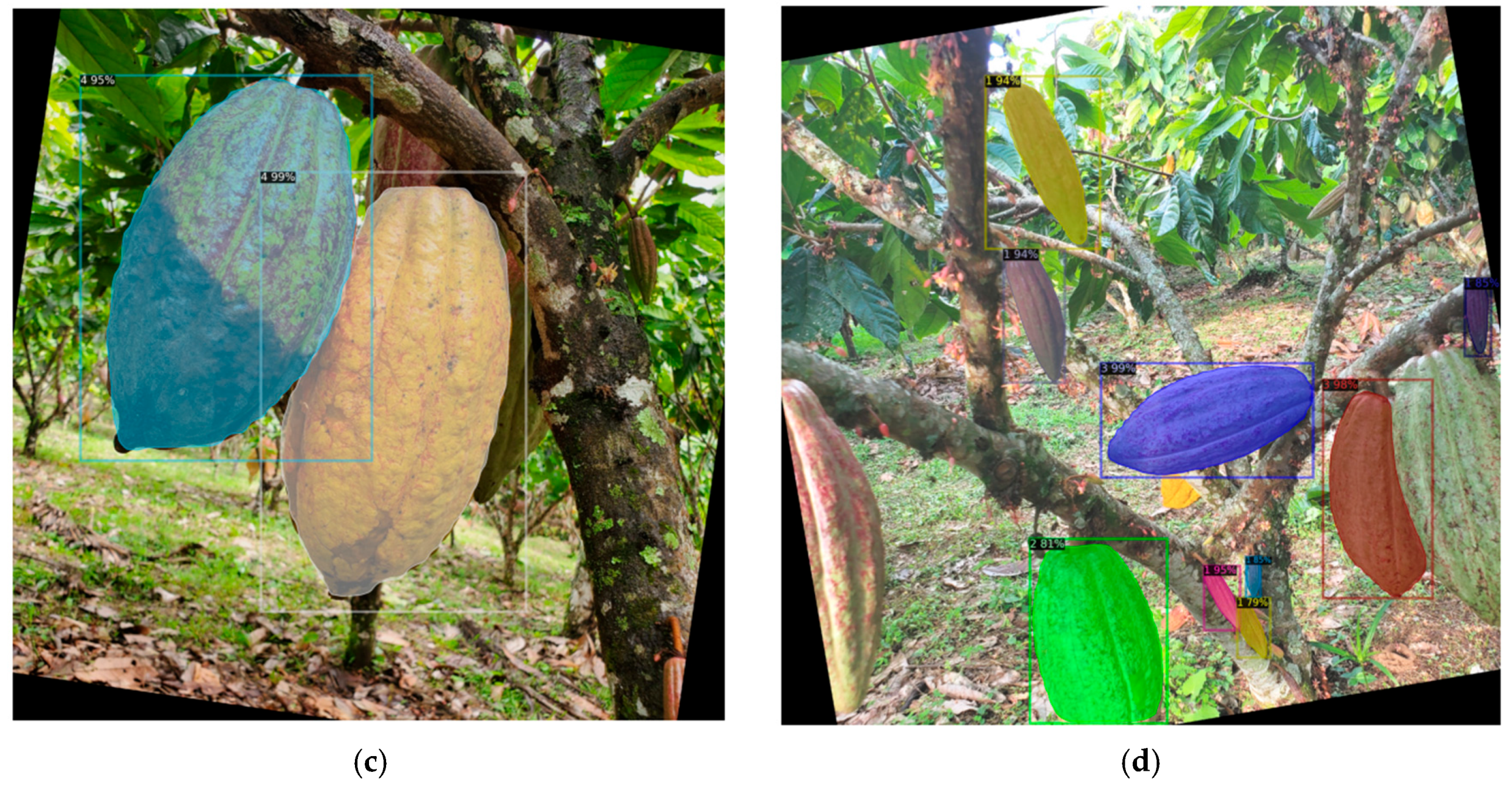
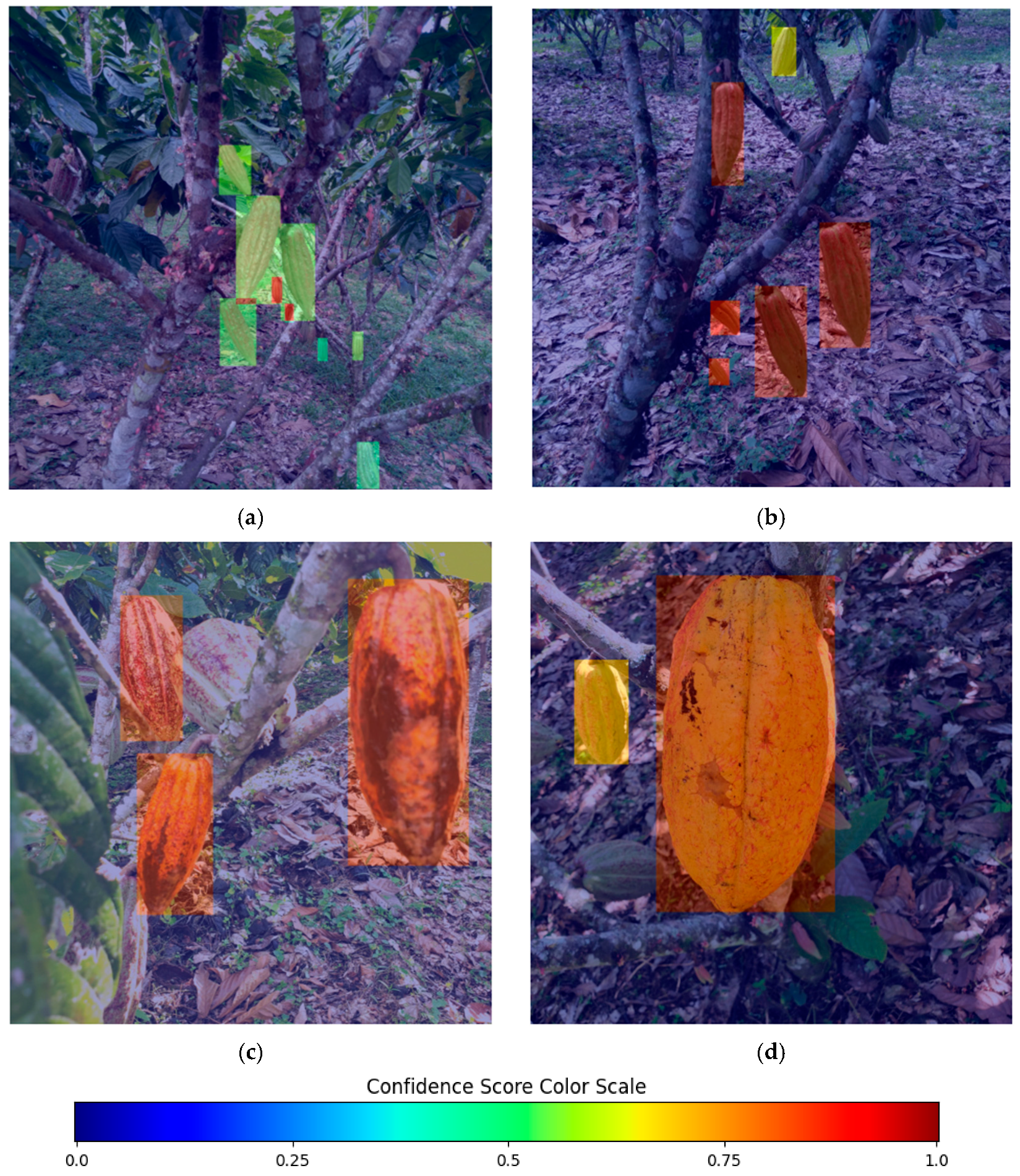
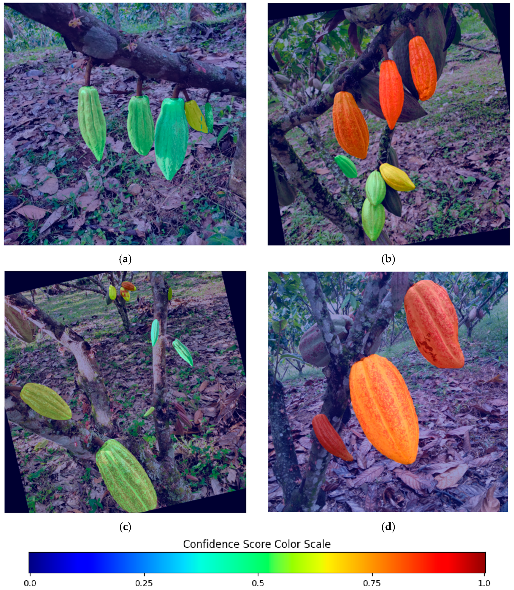
Disclaimer/Publisher’s Note: The statements, opinions and data contained in all publications are solely those of the individual author(s) and contributor(s) and not of MDPI and/or the editor(s). MDPI and/or the editor(s) disclaim responsibility for any injury to people or property resulting from any ideas, methods, instructions or products referred to in the content. |
© 2025 by the authors. Licensee MDPI, Basel, Switzerland. This article is an open access article distributed under the terms and conditions of the Creative Commons Attribution (CC BY) license (https://creativecommons.org/licenses/by/4.0/).