A New Approach to Topology Optimization with Genetic Algorithm and Parameterization Level Set Function

Abstract

In this paper, a new approach to topology optimization using the parameterized level set function and genetic algorithm optimization methods is presented. The impact of a number of parameters describing the level set function in the representation of the model was examined. Using the B-spline interpolation function, the number of variables describing the level set function was decreased, enabling the application of evolutionary methods (genetic algorithms) in the topology optimization process. The traditional level set method is performed by using the Hamilton–Jacobi transport equation, which implies the use of gradient optimization methods that are prone to becoming stuck in local minima. Furthermore, the resulting optimal shapes are strongly dependent on the initial solution. The proposed topology optimization procedure, written in MATLAB R2013b, utilizes a genetic algorithm for global optimization, enabling it to locate the global optimum efficiently. To assess the acceleration and convergence capabilities of the proposed topology optimization method, a new genetic algorithm penalty operator was tested. This operator addresses the slow convergence issue typically encountered when the genetic algorithm optimization procedure nears a solution. By penalizing similar individuals within a population, the method aims to enhance convergence speed and overall performance. In complex examples (3D), the method can also function as a generator of good initial solutions for faster topology optimization methods (e.g., level set) that rely on such initial solutions. Both the proposed method and the traditional methods have their own advantages and limitations. The main advantage is that the proposed method is a global search method. This makes it robust against entrapment in local minima and independent of the initial solution. It is important to note that this evolutionary approach does not necessarily perform better in terms of convergence speed compared to gradient-based or other local optimization methods. However, once the global optimum has been found using the genetic algorithm, convergence can be accelerated using a faster local method such as gradient-based optimization. The application and usefulness of the method were tested on typical 2D cantilever beams and Michell beams.

1. Introduction

Topology optimization is crucial in engineering because it enables the design of lightweight, strong, and efficient structures by optimally distributing material within a given domain, which is essential for applications such as aerospace, automotive, civil engineering, and additive manufacturing. The topology optimization process in structural mechanics aims to distribute material effectively to optimize load responses (bearing capacity). The literature on level set topology optimization encompasses several areas: geometry domain parameterization (SIMP [1], Level set [2]), interpolation methods (RBF, B-spline, NURBS [3]), equilibrium solving (FEM [1] and meshfree methods [4]), and optimization algorithms (gradient [1], non-gradient [5], evolutionary methods [6]).

Most existing methods rely largely on gradient-based optimization techniques, which tend to become trapped in local minima, especially for complex geometries. Furthermore, many of these approaches do not allow for the creation of new holes or topological features during the optimization process, which limits their ability to effectively explore the entire design space.

The process is primarily conceptual, with numerous papers ([1,3,7]) discussing various approaches and models. Effective shape parameterization is vital for geometry optimization. Traditional methods using FE node coordinates as shape variables led to numerous variables, gradient discontinuities, and challenges with mesh re-initialization. An alternative approach involves employing polynomials and parametric curves or surfaces, yielding a reduction in parameters introduced as optimization variables.

Various papers detail basic parameterization approaches and geometry modifications during optimization [8,9]. B-spline curves were utilized in parameterization and evolutionary methods, particularly genetic algorithms, which proved effective for shape synthesis ([8,9]). The homogenization method, which emphasizes mass distribution, is comprehensively detailed by Cappello and Mancuso [9], wherein genetic algorithms are employed to optimize material density to enhance stiffness while adhering to volume constraints.

However, such methods often require a high number of variables, especially with high geometric complexity, which affects the efficiency of the computation.

The complexity arises from solving displacement and geometry simultaneously, with critical reviews available [10]. The level set method has gained traction for efficiently changing model geometry. Introduced in [11], it allows dynamic adaptation, including 3D curve movement techniques [12].

Numerous studies have applied level set methods for contour description in various fields. The level set method, paired with RBF approximation, effectively describes implicit functions, facilitating geometry model adjustments through gradient optimization ([13,14,15]). A major limitation of gradient-based level set methods is their dependence on initial shapes and their inability to generate new topological features such as holes, making it difficult to explore more optimal configurations. Test cases, such as a 2D cantilever beam, employed RBF coefficients for surface change, permitting hole creation and merging during optimization based on the Hamilton–Jacobi transport equation.

In the work by Jia et al. [6], the evolutionary structural optimization (ESO) method combined with the level set approach enables novel geometries independent of initial configurations. Topology optimization of 3D structures utilizing genetic algorithms is discussed by Burczyński et al. [16], highlighting two parameterization methods: shape and material distribution. Additionally, the work by Ruiter and Keulen [17] introduces the Topology Description Function (TDF) method, utilizing genetic algorithms but maintaining high computational costs. Implicit TDF combined with level set methods allows for new hole creation during “Nucleation” optimization techniques presented in the paper [18].

While global optimization methods suit problems with fewer variables [5], studies focusing on parameterizing the level set method remain limited [19]. Interest in topology optimization within additive manufacturing has grown due to its ability to create complex geometries difficult for traditional methods. This optimization can enhance mechanical properties like stiffness and buckling resistance for specific manufacturing techniques (FDM, SLM) [20].

In most existing approaches, optimization relies heavily on gradient-based algorithms, which tend to become stuck in local minima and are unable to generate or modify topological features such as new holes or passages in the material on their own. This limitation restricts the search space, especially for complex geometries. Several evolutionary methods, e.g., [9], use homogenization theory in combination with genetic algorithms where the design variables are element densities, resulting in high dimensionality and computational complexity. Similarly, Ref. [6] proposes an evolutionary accelerated level set algorithm that combines ESO with level set methods and enables the automatic generation of new holes. However, such algorithms are often dependent on the initial topology and may have difficulties in finding the global optimum for complex structures.

The Smooth-Edged Material Distribution for Optimizing Topology (SEMDOT) method is developed within the context of meshless approximation in the paper [21].

In recent years, topology optimization has increasingly been applied to enhance additive manufacturing (3D printing) processes, aiming to improve material efficiency, mechanical performance, and design flexibility. Building on the advances in material modeling, paper [22] utilized structural analysis with a linear anisotropic material model within the topology optimization framework. Furthermore, a novel approach combining Rational Approximation of Material Properties (RAMP) and the Finite Element Method (FEM) was proposed in [23] to minimize peak stresses in multi-layer composite joints.

The work by Shin et al. [24] discusses using machine learning (ML) to mitigate conventional topology optimization (TO) computational costs. ML, especially deep learning (DL), accelerates the process and predicts optimal topology from intermediate stages, expediting time-consuming phases. The study by Deng and To [25] proposes a new parametric level set method utilizing deep neural networks (DNNs) to convert PDEs into parameterized ODEs for diverse designs. The integration of neural networks with genetic algorithms may significantly enhance data efficiency and solution quality in high-dimensional problems [26].

Topological optimization also has significant applications in civil engineering. Computer-aided methods have been developed for performance-based structural design, focusing on nonlinear pushover analysis—an inherently complex and iterative process [27]. The method targets 2D-braced steel frames, employing pushover analysis combined with optimization techniques, optimality criteria, and an ant colony metaheuristic algorithm to automate the design process. Its goal is to achieve optimal drift performance while minimizing total structural weight.

Another method applies a similar approach to reinforced concrete (RC) buildings, integrating pushover analysis with numerical optimization, optimality criteria, and an artificial bee colony algorithm [28]. This technique is used for the optimal design of concrete beams, columns, and shear walls.

In the context of civil engineering and structural design, the newly developed method presented in this paper complements existing approaches by introducing a robust topology optimization framework based on parameterized level set functions and genetic algorithms. It enhances the global search capacity and convergence speed (near global optimum), making it suitable for complex structural design problems where traditional gradient-based methods may struggle with local minima and initial solution dependency.

This paper presents an optimization method using a parameterized level set function with B-spline surfaces and genetic algorithms in MATLAB. Our research contributes to topology optimization, with potential acceleration through machine learning. DL, particularly convolutional neural networks (CNNs), could improve shape prediction and parameter optimization, enhancing both efficiency and accuracy.

A new topological optimization method, using genetic algorithms and B-splines, was tested on standard examples, reducing optimization parameters and dimensionality. Numerical efficiency benefits from substitution material formulations, eliminating remeshing. Maintaining a consistent range for objective functions and constraints is essential, using methods like standardization and logarithmic transformations to calibrate varying values. This paper introduces an extended objective function to enhance convergence with genetic algorithms and presents a novel penalty operator targeting similar individuals within each population generation, facilitating high-quality solutions in 2D topological optimization. The method presented in the chapter ‘Mathematical Formulations’ provides the detailed mathematical foundation and implementation details of this approach.

Most existing methods rely heavily on gradient-based algorithms, which tend to become trapped in local minima and generally do not facilitate the creation of new topological features such as holes or internal passages during the optimization process. As a result, these approaches often require favorable initial designs and have difficulty exploring the entire design space, especially for complex or highly non-convex structures.

The main contributions of this work can be summarized as follows:

• The proposed method uses a parameterized level set function in combination with genetic algorithms, enabling a global search that reduces the dependence on the initial topology.
• The method overcomes the limitations of local minima and allows topological changes, such as the creation of holes, during the optimization process.
• Although the method tends to have slower convergence rates, this can be mitigated by integrating local refinement techniques, including gradient-based fine-tuning or memetic algorithms, following the approximate identification of the global optimum.

These limitations can be observed in the images presented in the chapter, with the results.

2. Mathematical Formulations

2.1. Structural Topology Optimization

Typically, topology optimization problems involve minimizing compliance while considering displacement constraints and allowable material distribution, expressed using the material stiffness matrix E:

$$\begin{gathered} \underset{\begin{array}{c}\mathrm{u}\in \mathrm{U}\\ \mathrm{E}\in {\mathrm{E}}_{\mathrm{ad}}\end{array}}{\min }l\left(\nu \right) \\ {a}_B\left(u,\nu \right)=l\left(\nu \right), \mathit{for} all \nu \in U, E\in E_{ad} \end{gathered}$$

(1)

which represents a weak variation equation with U as virtual (kinematic permissible) displacements, where are E—stiffness matrix; $E_{ad}$—set of admissible stiffness tensors; $a\left(u,\nu \right)$—internal virtual work of an elastic body; $l\left(\nu \right)$—virtual work of external loads; $u$—equilibrium displacement field; $\nu$—virtual displacement (kinematic permissible) field. The index B indicates the bilinear form.

The linear form of the load $l\left(\nu \right)$ is the summation of the external load $f_v$ acting on the volume $\mathsf{\Omega }$ and the external load $f_s$ on boundary ${\Gamma }_s\subset \mathsf{\Gamma }\equiv \partial \mathsf{\Omega }$ (work of external load):

$$l\left(\nu \right)={\int }_{{\Gamma }_s}\nu ·f_s·d\Gamma +{\int }_{\Omega }\nu ·f_v·d\Omega$$

(2)

The internal virtual work of an elastic body can be expressed as follows:

$$a\left(u,\nu \right)={\int }_{\Omega }E\left(X\right)·\epsilon \left(u\right)·\epsilon \left(\nu \right)·d\Omega$$

(3)

where X is shape and topology variables (representing material distribution).

Linearized strain field are $\epsilon =L·u$, with L as the differential operator.

From virtual works, it becomes evident that by minimizing the bilinear form, we achieve the equilibrium state of the displacement field. This equilibrium of the bilinear form necessitates the optimization of material distribution to maximize stiffness:

$$\underset{E\in E_{\mathit{ad}}}{\mathit{max}}\left(\underset{uϵU,D}{\mathit{min}}\left\{a_B\left(u,\nu \right)-l\left(\nu \right)\right\}\right)$$

(4)

The objective function is the minimization of compliance to determine the optimal material distribution while ensuring equilibrium (using a nested approach). The formulation for minimum compliance in a discretized domain can be expressed as follows:

$$\begin{gathered} \underset{\mathrm{u},{\mathrm{E}}_{\mathrm{e}}}{\min }{f}^{T}u \\ K\left(E_e\right)u=f, E_e\in E_{ad} \end{gathered}$$

(5)

where u—displacement, f—load filed, K—stiffness matrix depending on material properties in element e ($E_e$). For N number of elements, the following applies:

$$K=\sum _{e=1}^N{K}_e\left(E_e\right)$$

(6)

$K_e$—element of global stiffness matrix.

The objective function can be expressed as a minimization of volume function with respect to the following stress constraints:

$$\begin{gathered} \underset{E_e}{\min }V \\ K\left(E_e\right)u=f, {\sigma }_e<{\sigma }_{ad} E_e\in E_{ad} \end{gathered}$$

(7)

We utilize a modified Level Set Method combined with the Topology Description Function (TDF). In dealing with shape-changing during optimization, two common methods for stress and strain calculations using FEM are substitute material method and remeshing. Due to the high computational cost of remeshing, we chose the substitute material method to significantly reduce computation time, applying it throughout all examples in this work.

2.2. B-Spline Parameterization of Level Set Function

The Level Set Method (LSM) relies on an implicit function that describes geometry. The level set function is an n + 1-dimensional function that represents n-dimensional geometry within an n-dimensional space through its isolines.

This characteristic of LSM allows for both geometry and topology changes during the optimization process. For instance, it can facilitate the creation of new holes within the domain without the need for establishing a new geometry parameterization.

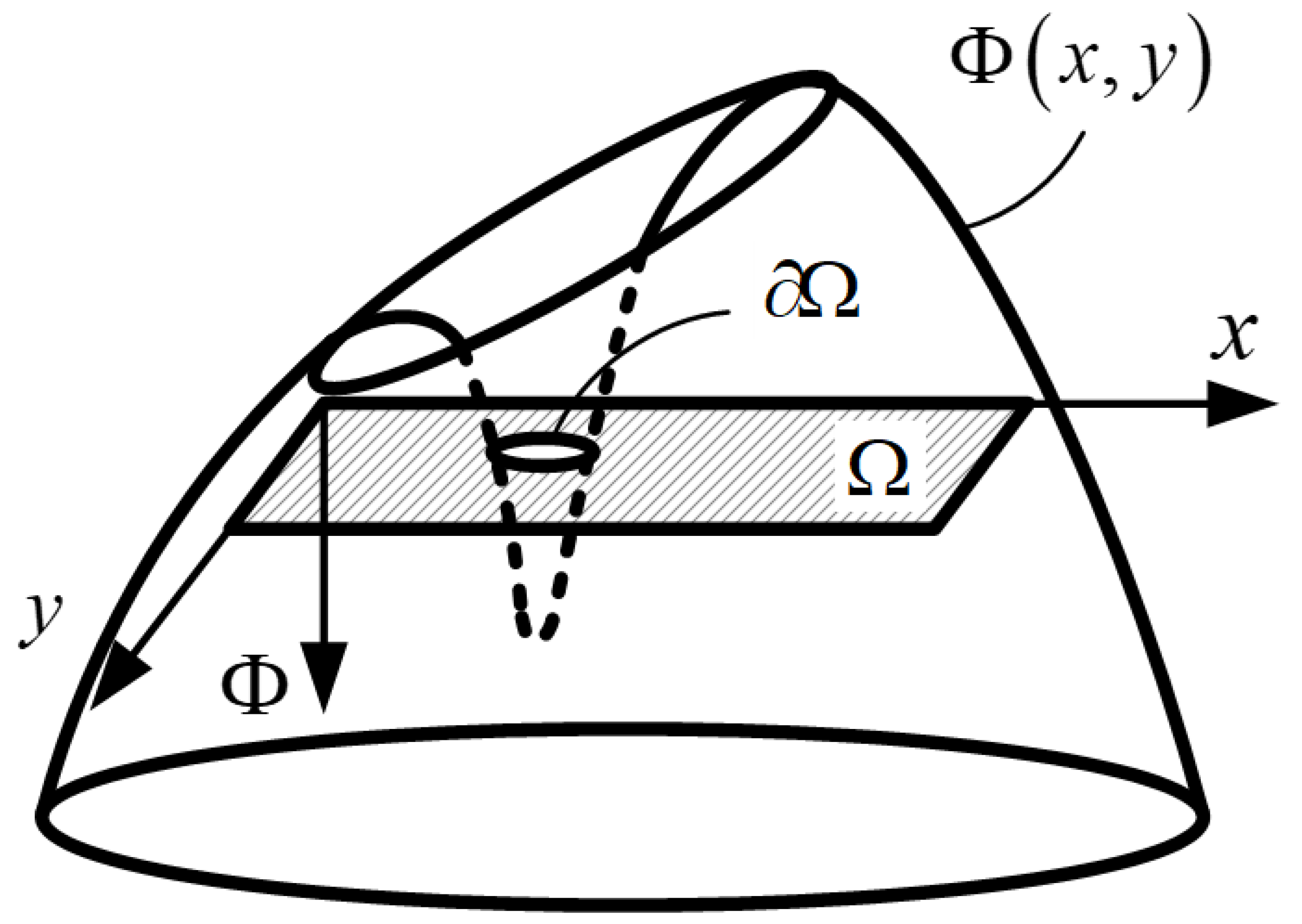
Figure 1 illustrates the 3D function $\mathsf{\Phi }$ (Level set function) used to describe the 2D problem. The level set function $\mathsf{\Phi }$ intersects the rectangular domain D (hatched area). When the rectangular domain D lies on the x-y surface, the cross-section of the function $\mathsf{\Phi }$ and the rectangular domain D together define a new domain $\mathsf{\Omega }\in \mathrm{D}$. There is a region with material defined as $\mathsf{\Phi }\left(\mathrm{x},\mathrm{t}\right)<0 \forall x\in \Omega \backslash \partial \Omega$, and region without material define as $\mathsf{\Phi }\left(\mathrm{x},\mathrm{t}\right)>0 \forall x\in \Omega \backslash \partial \Omega$. The zero-isoline of the level set function $\mathsf{\Phi }\left(\mathrm{x},\mathrm{t}\right)=0$ represent the contour $\partial \mathsf{\Omega }$, $\forall \mathrm{x}\in \partial \mathsf{\Omega }\cap \mathrm{D}$ on the x-y surface (boundary). Here, x denotes space variables. The change in the shape is numerically considered as a dynamical process, and it depends on the pseudo-time t.

The weight function H indicates whether the observed point is located inside or outside the following region:

$$H\left(\mathsf{\Phi }\left(\mathit{x}\right)\right)=\left\{\begin{array}{c}1 if \Phi \left(\mathit{x}\right)\le 0,\\ 0 if \Phi \left(\mathit{x}\right)>0,\end{array}\right.$$

(8)

The function $\mathsf{\Phi }$ is defined in 3D, while the observed shape is in 2D (i.e., in the n − 1 dimension). The isoline function $\mathsf{\Phi }$ at time t is currently as follows:

$$\mathsf{\Phi }\left(x,t\right)=0$$

(9)

All equations derived from expression (9) (such as the Hamilton–Jacobi equation) are only valid for the borders. However, the new approach to topology optimization involves the weight function H applied on a parametrized 3D B-spline surface, whose isoline represents the border of 2D geometry.

The B-curve is defined by Equation (10) through the points $P_i$:

$$P\left(t\right)=\sum _{i=0}^n{N}_{i,n}\left(t\right)·P_i,$$

(10)

where the basis function of the zero-degree B-curve is defined as follows:

$$N_{i,0}\left(t\right)=\left\{\begin{array}{cc}1,& t_i\le t<t_{i+1}\\ 0,& otherwise\end{array}\right.,$$

and, for the other degrees of the B-curve ($0\le i\le n+d$), as follows:

$$N_{i,j}\left(t\right)={\displaystyle \frac{t-t_i}{t_{i+j}-t_i}}{N}_{i,j-1}\left(t\right)+{\displaystyle \frac{t_{i+j+1}-t}{t_{i+j+1}-t_{i+1}}}{N}_{i+1,j-1}\left(t\right)$$

The degree of the curve falls within the range $1\le d\le n$, and each individual node is uniformly represented as follows:

$$t_i=\left\{\begin{array}{cc}0,& 0\le i\le d\\ {\displaystyle \frac{i-d}{n+1-d}},& d+1\le i\le n\\ 1& n+1\le i\le n+d+1\end{array}\right.$$

By multiplying two B-curves in x and y direction yields the 3D surface (B-spline):

$$P\left(u,v\right)=\sum _{i=0}^n\sum _{j=0}^m{N}_{j,d_n}\left(u\right)·N_{j,d_m}\left(v\right)·P_{ij}$$

(11)

Under this assumption B-spline surface (11) for n control nodes of the B-spline ($P_{ij}$), the interpolation of the implicit function can be written as follows:

$$\mathsf{\Phi }=\sum _i^n{\mathsf{\Phi }}_{\mathrm{i}}·P_{0i}={\mathsf{\Phi }}^T\left(x\right)·P_0\left(t\right),$$

(12)

Through Equation (11) (B-spline) and Equation (12) (level set function), the parameterized B-spline function is mathematically linked. In this process, the Pij optimization variable is defined, representing the priming variable P0, i.e., the variable that determines the shape of the B-spline surface and, ultimately, the topological structure.

All finite elements within the 2D domain D of the initial bearing structures, for which Equation (12) yields positive values, represent bearing elements with density ρ.

All finite elements within the domain located above the B-spline surface are designated as non-bearing elements, indicating a material density of zero. The number of variables used in traditional level set method optimizations was typically equal to the number of finite elements in the optimized structure.

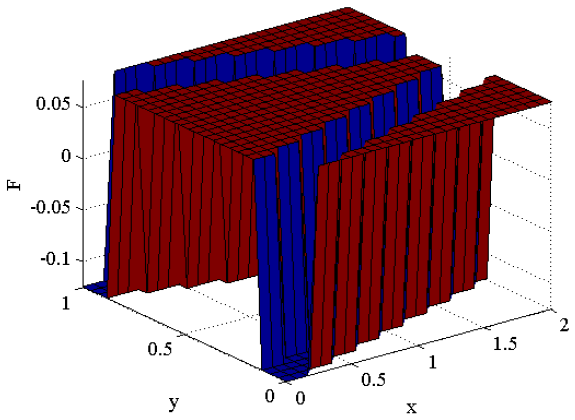
To assess the ability to describe geometry with a parameterized level set function, a step function with 676 control points is selected as the test function to be represented by a B-spline, as illustrated in Figure 2:

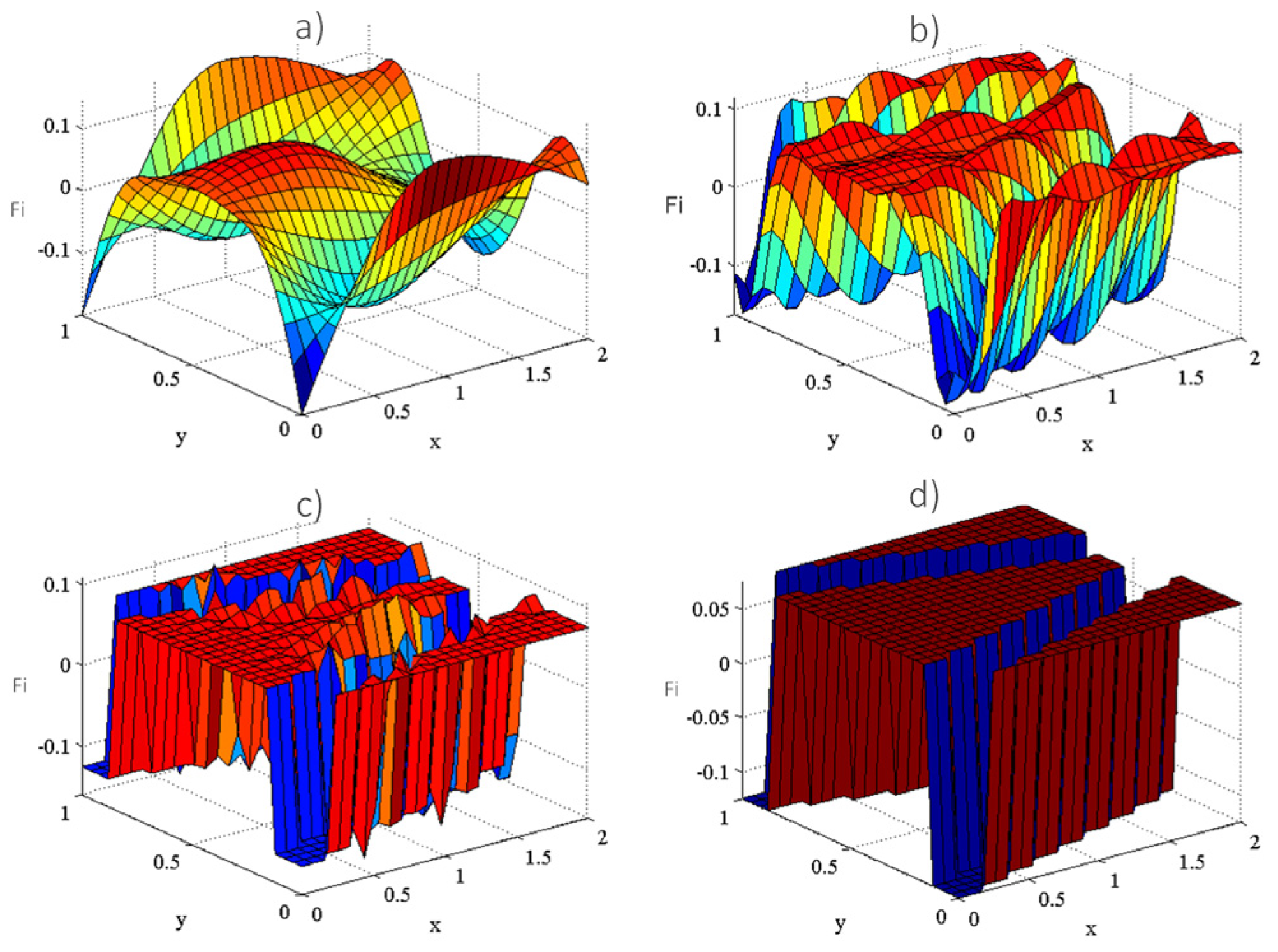
Appropriate parameterization of the level set surface using B-splines can significantly reduce the number of description variables, as illustrated by the results in

Table 1. Table of the influence of the node numbers and the degree of the B-spline.

B-Spline Nodes	2nd Degree	3rd Degree	4th Degree
	Error
6 × 6 (36)	1.457	1.504	1.517
12 × 12 (144)	0.415	0.417	0.429
24 × 24 (576)	0.0436	0.0405	0.079
48 × 48 (2304)	7.39 × 10−10	2.1 × 10−11	6.03 × 10−10

, and Figure 3.

In the optimization procedure for a beam, we used both 12 × 12 and 24 × 24 point grids to define the level set surface, resulting in 144 and 576 optimization variables, respectively. This larger number of variables helps mitigate the issues of local extrema that arise with fewer variables (36), necessitating a global search method like a genetic algorithm.

2.3. New Operators: Objective Function and Constraints

To achieve robust topology optimization results independent of the initial guess, we employed a genetic algorithm, an evolutionary global optimization method well-suited for finding the optimum of a function without becoming stuck in local optima. Our method modifies the traditional level set approach by allowing the creation of new holes, thus addressing its main limitation.

The functionality of this method was tested on cantilevers and Michell beams. We utilized a modified MATLAB finite element code based on Andreassen et al. [29] and Sigmund [30], employing a 2D finite element method for plane stress to analyze physical phenomena such as displacement, stress, and deformation.

Modifications included the incorporation of a B-spline parameterized surface, as described by Christensen [31], Equation (11), allowing the number of control points (P) to correspond to the number of optimization variables. This integration facilitated the use of objective functions and constraints to improve the optimizer’s sensitivity.

The objective function was formulated in two steps: minimizing compliance while respecting the volume constraint, Equation (5), and minimizing material volume under stress constraints, Equation (7).

To transform the discrete objective function into a continuous one, we introduced additional terms to enhance the optimizer’s sensitivity to variable changes, as shown in Equation (13):

$$F_c=B{r}_{elem}+\left(\sum \left|diff\left(Bspline\left(z\right)\right)\right|\right)$$

(13)

where $B{r}_{elem}$—number of elements that possess the mechanical characteristics of load-bearing structure materials, and $Bspline\left(z\right)$—values of the control points of the level set surface (F in Figure 2).

Furthermore, to improve convergence, we applied logarithmic transformations for stress constraints and utilized the arctangent function for deformation constraints. As stress values can reach magnitudes of 10⁷ MPa, a logarithmic transformation, Equation (14) was used to control these values within a range from 8 to 22.

$$Og{r}_{\sigma }=\sum _i^{n}log\left({\sigma }_i\right)$$

(14)

Excessive deformations were limited using the arctangent function, Equation (15), resulting in values now ranging from 0 to a maximum of 90, instead of very high values:

$$Og{r}_{\epsilon }=\sum _i^n\mathrm{a}\mathrm{r}\mathrm{c}\mathrm{t}\mathrm{a}\mathrm{n}\left({\epsilon }_i\right)$$

(15)

The optimization process began with an arbitrary design, focusing on minimizing the objective function. The findings highlight that the similarity in magnitudes of constraints facilitates their incorporation into a complex objective function, enhancing the optimization procedure’s effectiveness.

3. Numerical Examples, Results

To examine the proposed numerical procedure, several test examples were carried out. As described and examined in previous sections, we employed a uniform second-degree B-spline surface to describe the level set function during the topology optimization of a beam subjected to a 10 kN force applied to the right middle end.

The precision of the level set function representation by the B-spline was influenced by the number of control points. The z-coordinates of the B-spline nodes were treated as optimization variables. We selected two mesh sizes, 12 × 12 and 24 × 24 control points, for the B-spline surface. The total number of finite elements for all beam examples was 3200 (80 × 40).

The Young’s modulus of elasticity for the structural elements was set as $E=30 \left[GPa\right]$. In all tested examples, the maximum allowable Von–Mises stress was limited to 20 N/mm² to ensure the realism and safety of the structure. In the following figures, the colorbar displays the distribution of Von–Mises stress in N/mm². We conducted topological optimization of 2D cantilevers and Michell beams using a genetic algorithm. The number of elite individuals transferred to the next generation was 10. The recombination parameter for individuals was configured so that 80% of individuals from the previous generation (excluding elite individuals) underwent crossover using a random algorithm.

The mutation affected individuals who did not participate in the crossover, with approximately 5% of their chromosomes changed randomly (uniform mutation).

The range within which control points (optimization variables) could vary might influence the genetic algorithm’s convergence speed. In this case, the initial population range for optimization variables was selected between −2 and 2. We used real encoding for variables and the objective function during optimization with the genetic algorithm. All calculations were performed on a four-core Intel i5 3.10GH processor-based computer.

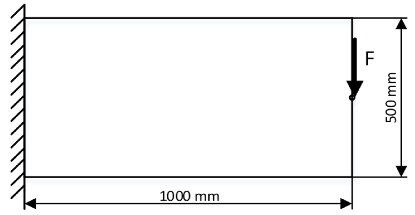
3.1. Test Case 1—Cantilever Beam

As a commonly used test case for topology optimization with the level set method, as documented in numerous references such as [4,13,32,33], a cantilever beam with a force acting at its free end was used, as shown in Figure 4:

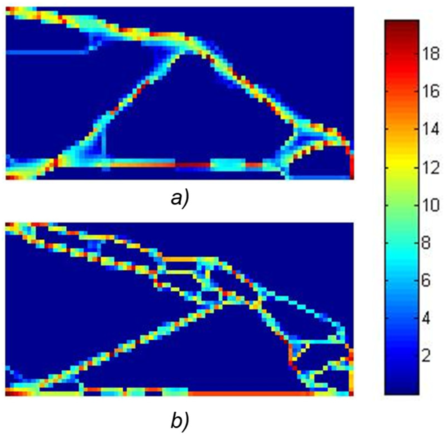
In this example, the objective function is set to the a minimum compliance, with the volume constraint at 20% of the initial design (640 elements), as shown in Figure 5:

Figure 5 shows the results of the test case 1 achieved using population of 5184 randomly generated individuals over 500 generations. The maximum Von–Mises stress was 20 [N/mm²], while the volume constraint was set at 640 elements, corresponding to 20% of the initial design. For 144 variables, the compliance was 6715 [Pa⁻¹], and the calculation time extended to 68 h. Remarkably, only for this case, 1000 generations were required to approach the global optimum (Figure 5a). In the case of 576 optimization variables, the objective function (compliance) amounted to 7776 [Pa⁻¹], with a calculation time of 42 h (Figure 5b). With fewer generations, the procedure yielded results that indicated local extrema, such as the optimum for the L/H ratio of 2.

For comparison, the minimum compliance according to [24], with the same parameters as in the previously described example Test case 1, is 5864 [Pa⁻¹]. We observe that the Evolutionary Algorithm did not converge to a solution; however, the proposed method came very close to the global optimum, which is the goal of the proposed approach.

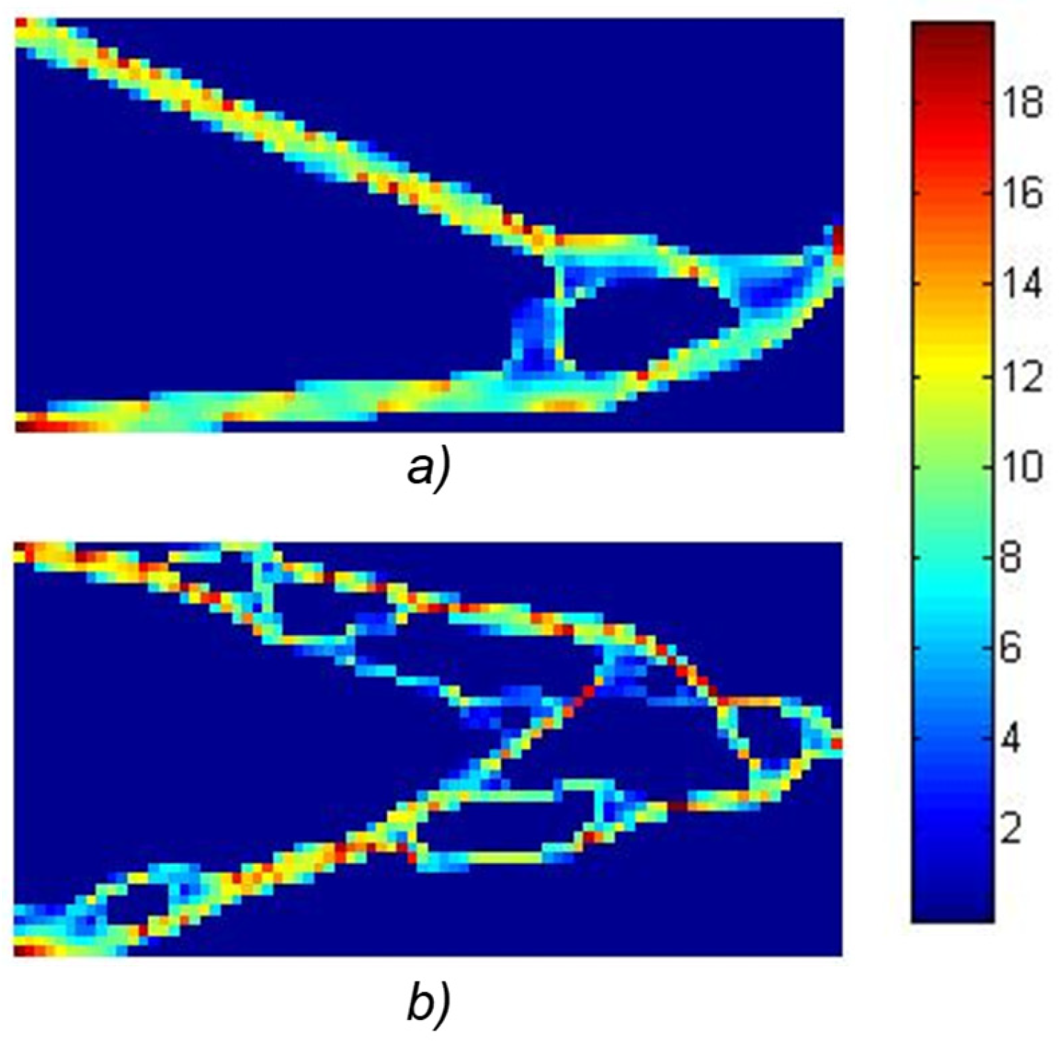
In the same test case, the objective function is formulated to minimize volume during topology optimization using the level set function and the genetic algorithm. We achieved the results as shown in Figure 6:

The results shown in Figure 6 represent optimal solutions obtained through the genetic algorithm procedure across 500 generations involving 5184 individuals. The computational process took approximately 35 h for 576 variables (Figure 6b), resulting in an objective function value of 657, corresponding to approximately 20.5% of the full plate volume. In the case of 144 variables, the objective function yielded a value of 663, with a calculation time of around 13 h.

As demonstrated in the preceding figure, achieving convergence was challenging. The genetic algorithm exhibited slow convergence in the vicinity of the solution. Therefore, the obtained results can serve as initial solutions for the gradient method, which offer fast convergence but may converge to local optima. This optimization approach grants the optimizer flexibility in generating the geometry and the capability to discover global optima.

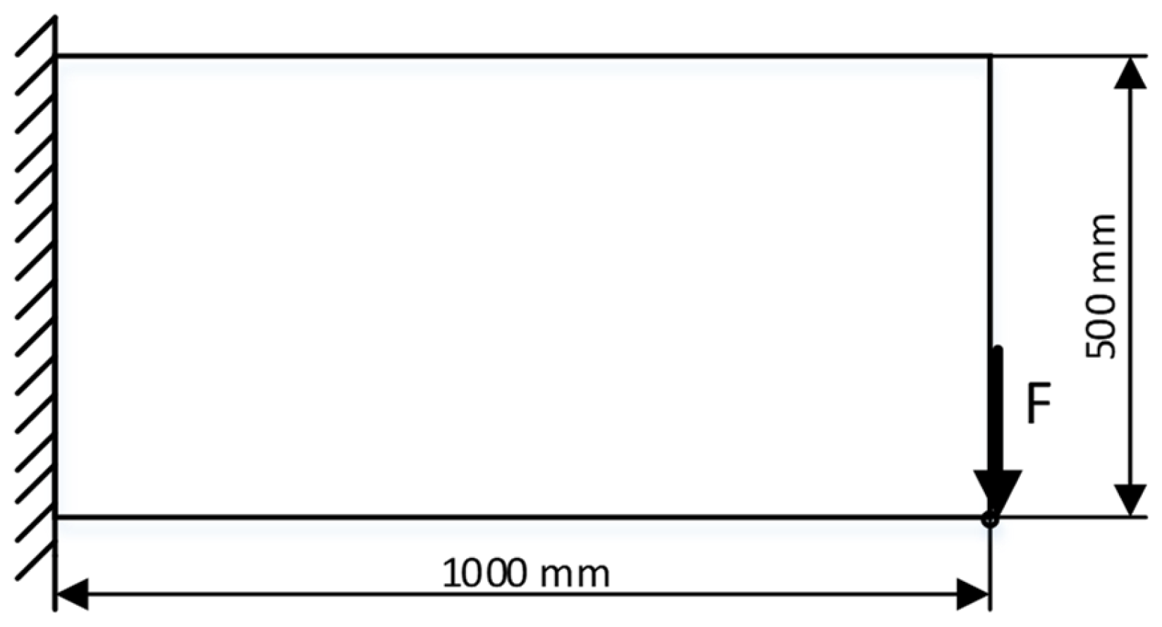
3.2. Test Case 2—Cantilever Beam

The second test example is also a cantilever beam with a force acting on the lower edge at its free end, as shown in Figure 7:

In the provided example, using the same parameters (such as force, material properties, genetic algorithm parameters, allowable stresses, etc.) as in the previous case, we applied the 2D level set method for topology optimization of a cantilever beam subjected to force at its free end, on the bottom side of Figure 8.

The proposed method with 144 optimization variables, targeting a volume of 20% of the initial volume (640 elements) with the specified genetic algorithm parameters, failed to converge. However, when targeting a volume of 30% of the initial volume (960 elements), the objective function (compliance) reached 4147 Pa⁻¹ Figure 8a). In the case of 576 optimization variables Figure 8b), and a target volume of 20% of the initial volume, the compliance reached 8519 Pa⁻¹.

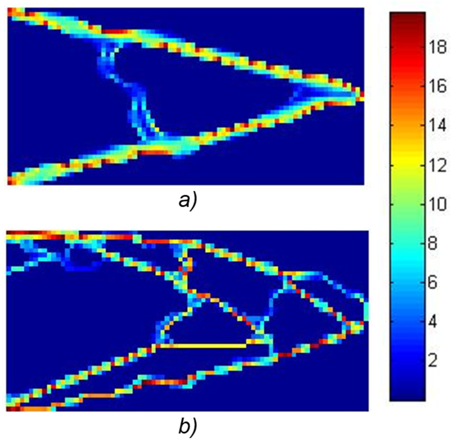
Again, a comparison with the work of [24] was conducted for Test case 2, where the minimum compliance with the same parameters is 3968 Pa⁻¹. It can be observed that the Evolutionary A more significant deviation from the optimal solution was observed precisely in the example with a higher number of variables. However, the primary goal of this study was to assess whether the proposed method is capable of finding the global minimum, which has been confirmed by the presented results. Future work will focus on developing a comprehensive topological optimization method that reliably identifies the global extremum. In formulating the objective function to minimize the volume of the cantilever beam (Figure 7), the following results were obtained (Figure 9):

In the second example of optimization using the proposed procedure with 144 optimization variables Figure 9a, the volume was reduced to 22% of the initial volume (707 elements). When increasing the number of optimization variables to 576, the volume was further reduced to 19% of the initial volume (614 elements). The parameters of the genetic algorithm and the allowed stress remained the same as in the previous example.

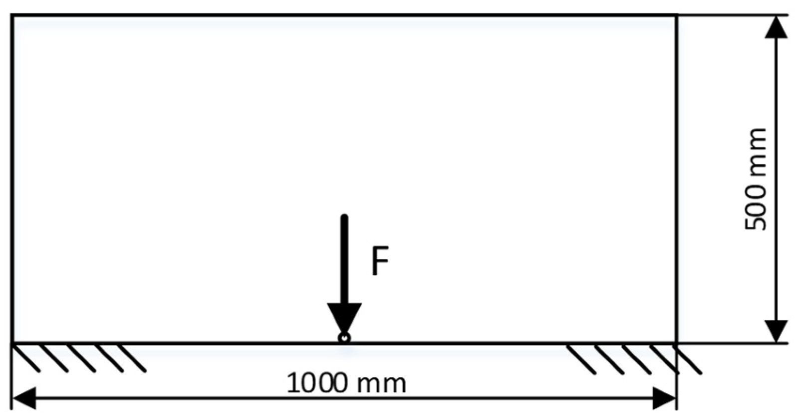
3.3. Test Case 3—Michell Beam

In the example illustrated in Figure 10—Michell beam, the objective function was set to minimize compliance while maintaining a volume constraint of 15% of the full plate.

The conditions for this optimization remained equal to those in the previous two examples, including parameters of the genetic algorithm and allowed stress. This led to the successful optimization of the Michell beam using the level set method, as demonstrated in Figure 11.

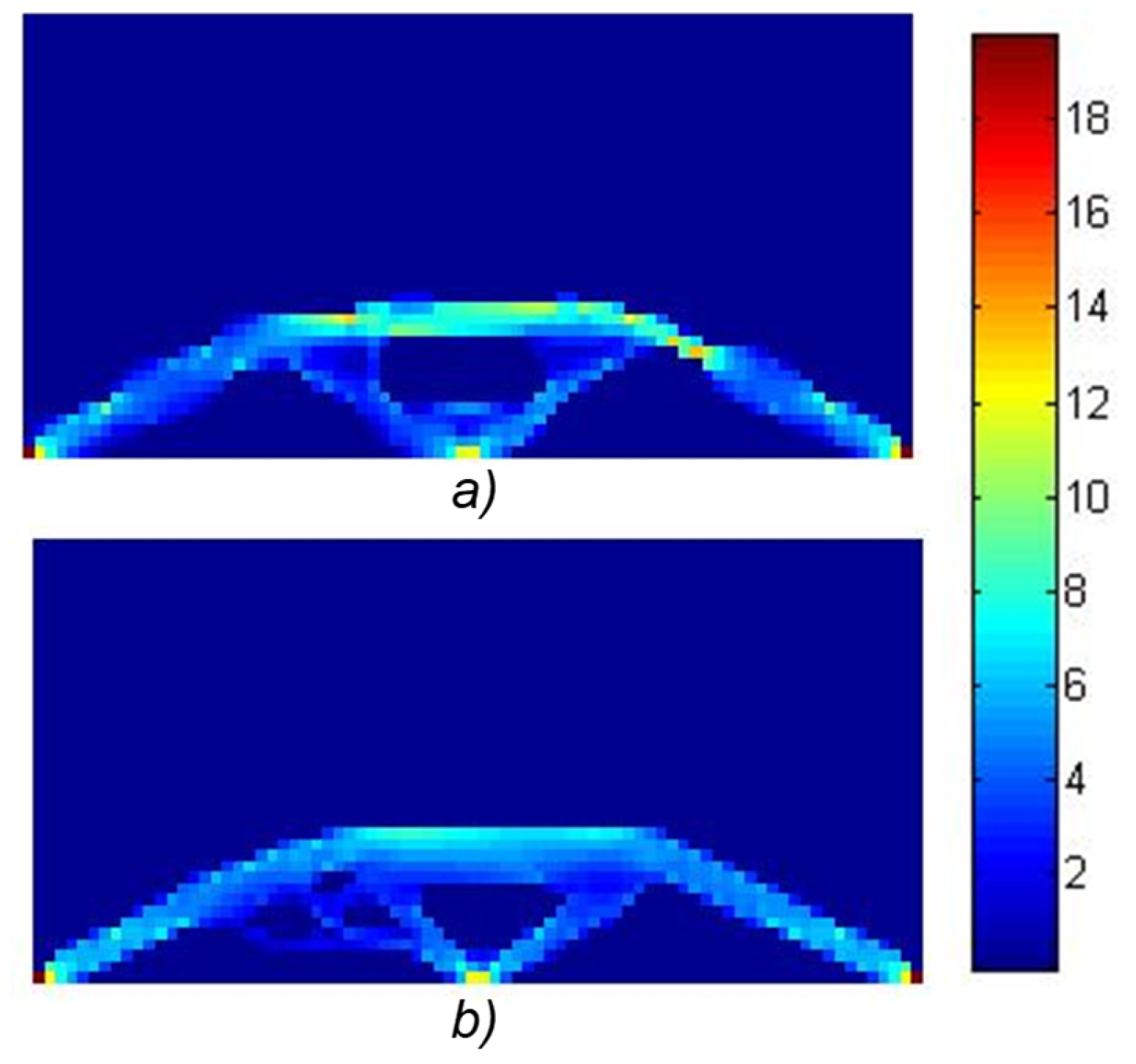
In the case of 144 optimization variables, for a specified volume of 15% of the initial volume (480 elements), with a population size of 5184 individuals and 200 generations of the genetic algorithm, convergence to a solution was achieved, as shown in Figure 11a, with a compliance objective function value of 1639 Pa⁻¹. When employing 576 optimization variables (as shown in Figure 11b), along with an increased number of generations set to 500, while maintaining the same parameters as in the previous example with 144 variables, a compliance objective function value of 1437 Pa⁻¹ was achieved. For test case 3, the minimum compliance according to [24], with the same parameters, is 996 Pa. As with the previous cases, the Evolutionary Algorithm did not fully converge to an exact solution; however, the proposed method achieved a result very close to the global optimum, fulfilling the primary objective of the approach. It is expected that in complex geometries and more challenging problems, the proposed method will be capable of finding the global minimum, since traditional topological optimization methods, such as those in [24], tend to be significantly influenced by the initial solution. In contrast, the proposed approach does not have such dependence, thereby increasing the likelihood of reliably locating the global extreme in complex scenarios. Therefore, the results confirm the method’s capability to approximate the global minimum, supporting the ongoing development of a comprehensive topological optimization procedure that can reliably detect the global extreme in future research.

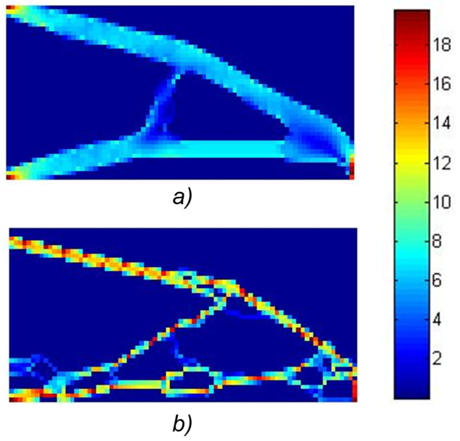
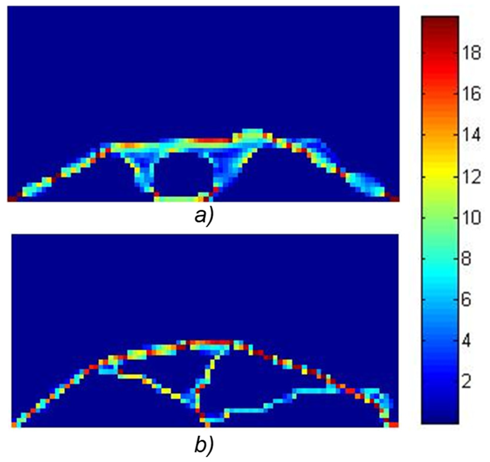
Regarding the formulation of the objective function for minimizing the volume of the Michell beam (Figure 10), the following solutions were obtained (Figure 12):

In the context of minimizing volume for the Michell beam example, optimization with 144 variables reduced the volume to 15% (354 elements) of the full plate, as illustrated in Figure 12a. When employing 576 variables, the volume was further reduced to 8% of the initial design (261 elements), as shown in Figure 12b.

The results demonstrate that a higher number of variables in the optimization process contributes to better convergence towards the global optimum, especially for structures with complex geometries. This is reflected in a finer and more precise material distribution, which allows for more efficient utilization of material resources and a reduction in the overall compliance of the structure. On the other hand, optimization with a smaller number of variables, while potentially enabling a faster identification of the global solution for less complex geometries, often requires the use of alternative methods or numerical techniques to achieve convergence towards a high-quality solution, since it may struggle to accurately represent intricate designs. The uneven stress distribution in the elements is primarily a consequence of the slow convergence towards the optimal solution when employing a global optimization method such as a genetic algorithm. While the addition of a penalty term to the objective function, designed to penalize similar individuals and promote diversity, has certainly improved the method, reaching the ideal optimum as presented in the extensive literature referenced in the introduction [1,3,13], etc., remains challenging. Furthermore, the method’s functionality was validated against an analytical solution for a length-to-width ratio of 1:1, where the method successfully identified the optimal solution. It is crucial to emphasize that the proposed method consistently achieves solutions that are very close to the global optimum, regardless of the initial starting solutions. This robustness is a significant advantage.

From the obtained results, we can see that the proposed method can be used as a generator of good initial solutions close to the global optimum for conventional methods for topology optimization.

4. Discussion

This study presents a novel approach to topology optimization using a parameterized level set function and genetic algorithms. The method demonstrates promising results in finding global optima, particularly when dealing with complex structures. The use of B-spline surfaces reduces the number of optimization variables, enhancing the efficiency of the genetic algorithm.

This paper also introduces a novel penalty operator designed to enhance convergence and ensure good sensitivity in the optimization process. While the penalty operator alone did not significantly improve convergence, when combined with the extended objective function, it facilitated the generation of high-quality solutions.

The presented method shows potential for accelerating the optimization process and finding more accurate solutions, but faces challenges related to computational cost, particularly when dealing with complex structures and large numbers of variables. Genetic algorithms, while effective for global search, can be computationally expensive. Future research should tackle these limitations by integrating the proposed approach with gradient-based optimization and exploring machine learning techniques for better efficiency and scalability. Additionally, applying the approach to 3D problems is worth investigating.

Topology optimization with the proposed method provides the advantage of finding good initial solutions for other topology optimization procedures, such as SIMP, ESO, and LS, where the selection of suitable initial solutions is crucial for convergence.

It is worth noting that very few papers address the formulation of minimum mass with stress/strain constraints in topology optimization using gradient-based procedures, mainly because achieving satisfactory results often relies heavily on having an excellent initial solution.

In this paper, a novel method for topology optimization, which combines a level set function with a genetic algorithm, is introduced. The developed optimization procedure was implemented using a custom MATLAB code based on the SIMP method for topology optimization, as described in references [29,30]. It is important to note that this code is specifically designed for 2D problems. The results of this study demonstrate the method’s capability to discover effective solutions for structural optimization tasks.

The results obtained demonstrate convergence to the global optimum in all examples, even with a smaller number of generations. Consequently, the proposed evolutionary topology optimization method can be employed as a generator of high-quality initial solutions for more computationally efficient gradient-based procedures.

The limitation of this proposed method is the duration of the optimization. However, considering that the method is based on the genetic algorithm, it is amenable to parallelization, which has the potential to significantly reduce the optimization time. In a study by [34], it was demonstrated that geometry optimization could be efficiently carried out using an ad-hoc cluster, resulting in a reduction in processing time proportional to the number of services.

During topology optimization using the proposed method, it was observed that at smaller numbers of individuals per generation, the optimizer identified local optima, leading to premature convergence of the genetic algorithm. Premature convergence can occur due to the following:

-

Poor sensitivity of the objective function;

-

Instances where multiple individuals produce the same objective function value (resulting in reduced population).

To improve the convergence of the genetic algorithm, an additional penalty operator can be introduced to penalize equivalent individuals during the optimization process. Equivalent individuals receive a specific penalty added to their objective function, promoting greater diversity within the population. In our study, we also conducted tests on penalizing similar individuals to increase diversity; however, this penalty did not contribute to faster convergence of the optimization process.

5. Conclusions

This paper presented a novel approach to topology optimization that integrates a parameterized level set function with genetic algorithms, demonstrating promising capabilities in identifying global optima for complex structures. The use of B-spline surfaces not only reduces the number of optimization variables but also enhances the efficiency of the genetic algorithm, yielding high-quality solutions.

While various penalty operators were investigated to improve convergence and sensitivity, the proposed set of operators proved effective in achieving convergence and generating high-quality solutions. When combined with the extended objective function, this method demonstrated significant potential for enhancing topology optimization processes. However, challenges remain, particularly regarding the computational costs associated with complex structures and large variable sets.

Furthermore, integrating machine learning and deep learning methods could further enhance the optimization process and scalability. Expanding the applicability of the method to 3D problems also represents a significant area for future exploration.

The proposed topology optimization method plays a crucial role in providing effective initial solutions for existing procedures such as SIMP, ESO, and LS, where selecting appropriate initial conditions is vital for achieving convergence.