1. Introduction
Queuing theory is an effective mathematical instrument for optimally scheduling restricted resources in a wide range of real-world systems and networks, like contact centers, manufacturing and logistical systems, wired and wireless telecommunication networks, healthcare, emergency help, administrative systems, banks, etc.
A lot of the research that has been carried out on the edges of queuing theory has focused on creating and using methods to analyze and improve systems that have a fixed configuration, such as a set number of channels, buffer capacity, and admission and service rules, as well as a fixed pattern of arrivals, service, retrials, breakdowns, repairs, impatience, and other processes. However, in many real-world systems, these configurations can vary over time. In particular, the information arrival rate is usually not constant during a day, and the transmission rate in many wireless networks may essentially vary due to various reasons (noise, interference, rain, fog, obstacles in the transmission thread, etc.). An important class of queuing models that account for the fact that the parameters of a system can randomly vary during its operation are so-called queuing systems operating in a random environment (). Usually, we refer to an as an external random process that influences the parameters of a queuing system. Usually, this process is Markovian (sometimes semi-Markovian) with a finite state space. The jump of an between states implies the instantaneous change in certain parameters of the distributions characterizing the system’s dynamics.
Motivation of the necessity of investigating queues operating in an RE. The simplest examples of queues operating in an (s) are unreliable queues, where one of the two states of the corresponds to the system’s working state, and the second state corresponds to the system state when the channels can be broken. Another trivial example of s is queues with a Markov arrival process () and/or a phase-type () distribution of service times. The directing process of arrivals and/or services plays the role of an in these examples. It is more common to speak about a when more than one directing process is influenced by the and when the jump of the process has a synchronous impact on the directing processes, e.g., simultaneously on the directing processes of service and arrivals.
Because the standard assumption that the system’s parameters are fixed and not altered during system operation is quite artificial, rarely holds in real-world systems, and is imposed only to make the analysis simpler and obtain nicer analytical or algorithmic results, it is evident that the investigation of s is significant for queuing theory, as well as its applications. This explains why the analysis of s has quite a long history.
A short overview of the relevant literature. As the earliest work in the field of
s, the works cited in [
1,
2,
3,
4,
5,
6] can be mentioned. A brief history of the theory of
s, a list of references, and examples of the application of
s in real-world systems are presented, for example, in the publications cited in [
7,
8,
9,
10,
11,
12,
13,
14,
15].
Most of the findings that have been obtained for s relate to the queues having a single channel or infinitely many channels. To simplify the survey of the existing extensive literature, we will mention here only publications related to the analysis of s that are closest to the system considered in our paper.
In particular, we mention only papers devoted to multi-channel queues having a finite number of channels larger than one.
QOREs with a Markov arrival process and phase-type service time distribution. Here we limit our study to the investigation of systems where the service time has a phase-type (PH) distribution and the arrival flow is characterized by a Markov arrival process (MAP) in a given state of the RE; see, e.g., [
6]. This decision is justified as follows.
A stationary Poisson arrival process that has been extensively explored in the literature over the years is already acknowledged to be inferior to the as a model of actual arrival processes. The was introduced by M. Neuts as a versatile arrival process.
The
allows fitting not only the mean arrival rate (or inter-arrival time) of a real flow, e.g., information flow in telecommunication networks, but also the values of the variance and higher moments and the possible correlation of inter-arrival times. The
is able to capture characteristic properties of arrival processes in contemporary communication networks and contact centers, such as overdispersion and positive correlations between arrival moments. This has made popular the use of the
for modeling real-world flows. For further details on the
, its attributes, and particular cases, see, e.g., [
16,
17,
18,
19,
20].
The phase-type
distribution (see [
6,
21,
22,
23]) is the essential generalization of the exponential distribution for which the analysis of queues with such a distribution in an analytical form is still possible. In contrast to the exponential distribution, which allows fitting only the expectation of a random variable, the
distribution allows fitting also the higher moments, the variance in particular.
The choice of the distribution for characterization of service times in real-world systems is justified by (i) the relative simplicity of the analysis of queues (especially multi-channel queues) with such a distribution, compared to the analogous systems with an arbitrary distribution, and (ii) the suitability of this distribution in order to suit any given distribution.
In the papers [
8,
9], an
retrial
with a finite source of requests is considered. In ref. [
8], the existence of an additional
arrival process for negative requests is supposed. In ref. [
8,
9], the analysis of the systems is implemented via consideration of a
with the finite state space. The stationary probabilities of the
are calculated. Primary performance metrics are acquired, and numerical examples are given.
In paper [
11], a
type
with retrials is investigated. The system lacks a buffer. When a request is unable to catch a free channel upon arrival, it is still able to try again to obtain a service by retrying from orbit. It is suggested that the
state also affects the rate of repeated attempts. In contrast to [
8,
9], the state space of the considered
in [
11] is infinite. Deriving a condition for the existence of the
’s stationary distribution becomes necessary as a result. The stationary distribution is computed, and the sufficient condition for ergodicity is proven. The numerical experiment’s findings demonstrate that simpler queuing models do not accurately represent the system’s key performance metrics. Both the impact of the retry intensity and the potential for traffic smoothing are displayed.
The above-mentioned models assume that all requests belong to one class. In some real-world setups, requests can be heterogeneous, having various requirements for service and different priorities. In ref. [
24], a
type
with two types of requests is under study. Under the fixed state of an
, the arrivals occur in an
(marked Markov arrival process); for details, see, e.g., [
25,
26]. One of the two types has non-preemptive priority.
In [
27], an
inventory-
was considered. Service to a request can be implemented only when there are inventory units that are stored in a storage facility of finite capacity.
QOREs with a varying number of channels. Most of the existing papers on multi-channel s do not assume a change in the number of channels. Such a change is supposed to occur in the unreliable multi-channel queuing systems, where channels can be broken and require repair. As a result, a random number of channels can be available at an arbitrary time.
However, usually, a simultaneous random change in the number of available channels and rates of the arrival flow and service process is not suggested. This is a significant flaw in the body of the current literature from the point of view of potential applications. This is because it is evident that an effective system manager has to immediately react to the increase or decrease in the arrival or service rate by appropriately increasing or decreasing the number of channels providing service. Consequently, the account of the potential to alter the number of channels along with changes in the traffic rate and service rate is vital for making correct managerial decisions. Unfortunately, the existing literature devoted to the analysis of
s with a variable quantity of channels is sparse. Only studies in [
28,
29] where the arrival and service process characteristics, as well as the number of accessible channels, are changed simultaneously with the state of an
changing can be mentioned.
In ref. [
28], an
type
is under study. The number of channels, arrival, service, and impatience rates for requests are among the system’s characteristics that are contingent on an
’s state and fluctuate in value throughout its leaps. The dynamics of the system are determined by a multidimensional asymptotically quasi-Toeplitz
(
), see [
19]. Using the results for
s, a steady-state distribution computation algorithm is given, along with the derivation of an ergodicity criterion. The system’s primary performance metrics are computed.
A variation in the number of channels was also assumed in the paper [
29]. An
type
with heterogeneous requests and non-preemptive priority is analyzed. In addition to the available number of channels, the thresholds defining the strategy of channel reservation for priority requests depend on an
as well.
Models considered in [
28,
29], and several other papers of the authors of this paper assuming the possibility of a random alternation of the channel number are valuable from the perspective of solving a wide range of problems in the examination of different real-world systems. The well-known occurrence of hours of low, intermediate, and peak load in communication and transportation networks explains fluctuations in the intensities of request arrivals and retrials in real-world systems, including contact centers, supermarkets, etc. Alternation of the number of channels and service rates can be triggered by the change in the bandwidth currently available for transmission and the used modulation schemes.
Contributions of the paper. The paper’s contributions consist of an exact algorithmic study of a more advanced model compared to [
28], where the dependence of a channel number on the state of an
is also assumed. The two essential advantages of this model are as follows.
In the listed models, the exponential distribution of service time, at a given state of an
, is assumed. Here, we suggest that such time has an essentially more general
distribution. The reason for the consideration of only the exponential distribution in [
28] is the following. The possibility of a random change in the channel number implies the necessity to sometimes break ongoing services or, conversely, to start several new services. When the service time is exponentially distributed, due to the famous memoryless property of this distribution, it can be carried out rather easily. In the case of a
distribution, essential difficulties arise due to the need to account for, along with transitions of directing processes in busy channels, additional transitions of these directing processes caused by the alternation of the channel number. Because of the potential for huge block sizes in a generator, there are challenges when constructing the
’s generator explicitly, as well as when implementing the computation of the stationary distribution using a computer. Here, we succeeded in overcoming these difficulties.
In the existing papers, it is suggested that in every state of the the state space of the directing process of the is permanent. The state of this process is not changed at the jump moment of the . Only the intensities of transitions in the directing process become different after this jump. Oppositely, we assume that the directing process may jump at the moment of the jump of the Accordingly, in various states, the state spaces of the directing process may have different cardinalities. An account of this possibility is important for applications because traces of real traffic at different states of the can be fitted by the s of different dimensions. For example, in some states, when inter-arrival times have a low correlation and a coefficient of variation of about 1, the flow may be fitted by a stationary Poisson process. In other states, when inter-arrival times have higher correlation and variation, the flow may be fitted by an . A more adaptable and sufficient model of the arriving process in the actual world may be constructed by taking into consideration the flexibility of the cardinality of the state space of the directing process.
Possible applications of the model. Some potential applications of s are as follows.
Various systems for the transmission of heterogeneous information. Certain kinds of data are tolerant of partial losses yet extremely sensitive to jitter and delay. Some other varieties can handle delays, but they become sensitive when a packet is lost. Elastic traffic can tolerate bandwidth fluctuations, but non-elastic traffic needs a steady bandwidth. As a result, several systems for dynamic bandwidth sharing across various information types are constantly evolving. They make the assumption that transmission of the delay-tolerant flows is delayed in the event of congestion to improve circumstances for delay-sensitive flows. A probabilistic analysis of the random processes describing the transmission process of various flows is necessary for the study of such systems. The intricacy of the mathematics frequently makes this analysis unfeasible.
Various systems with varying service rates. Such a fluctuation may result from the transmission thread’s random deterioration for technical reasons, as well as from external factors including weather, inversions in the atmosphere, interference, noise from enterprises and transportation, users’ mobility within a cell using different modulation techniques based on how far they are from a base station, etc.
Hybrid Free Space Optics/Radio transmission channels. In recent years, free space optics (
) technology has been extensively employed; for example, see [
30,
31]. The foundation of this technology is the transmission of data via the atmosphere using modulated radiation in the visible or infrared spectrum, followed by an optical photodetector device’s detection of the data. The two primary benefits of an optical communication link are (i) excellent digital communication quality and bandwidth and (ii) good channel security against stealth and illegal access.
Consequently, laser systems are frequently employed for diverse applications necessitating high data transmission confidentiality, as well as elevated noise immunity and non-interference.
The technology has two major disadvantages in addition to its advantages: (i) the channel’s accessibility is weather-dependent, and (ii) direct sight between a transmitter and a receiver is necessary. The range of a laser atmospheric communication line can be significantly reduced by unfavorable weather conditions like snow or fog. Therefore, to achieve acceptable dependability values for an communication channel, hybrid approaches are required.
The foundation of a hybrid radio–optical technology is the combination of an optical channel with redundant radio channels operating in the centimeter and/or millimeter range of radio waves. The weather has essentially no effect on how the radio channel operates in the centimeter band of radio waves. Fog has no effect on a millimeter-wave wireless channel’s performance. At the same time, severe rain significantly lowers the signal/noise ratio, which is a measure of how well a channel performs. The complementary characteristics of broadband radio channels and optical channels have allowed for the development of hybrid carrier systems, which are capable of dependable operation in all weather conditions.
In response to the significant need for high-speed and stable communication channels, several architectures of hybrid systems are employed to address the “last mile” issue. They utilize a high-speed laser channel allocated by a broadband radio channel functioning under the IEEE 802.11n protocol within the centimeter band of radio waves; a radio channel in the millimeter-wave E-band (71–76 GHz, 81–86 GHz); and a parallel-operating radio channel in the millimeter band reserved by an IEEE 802.11n channel. The functionality of such channels in diverse meteorological situations is accurately delineated by s.
Technologies 5G and 6G New Radio, in which significant variation of transmission rates may occur due to a dynamic blockage of propagation paths by various blockers (vehicles, human bodies, etc.) and the multipath transmission, see, e.g., [
32,
33,
34,
35].
Wireless local area networks serve people living in a certain area, such as a collection of buildings. It is popular among residents to use, along with access to external resources, the relatively inexpensive access to service provider’s internal resources, including computer games, music, video, and multimedia. A provider can collect statistics about the rate of generation of user requests that may essentially vary during the day and nighttime (which can be interpreted as the influence of an ). A provider may control the cost of access by raising it during times of high demand and lowering it at times when the servers (and wireless channels for access) are not being used to maintain a high standard of customer care. This should make the traffic smoother and increase the revenue of the service provider.
Wireless sensor networks with energy harvesting are designed for different needs, e.g., providing security for some objects. The rates of signal generation from the objects may fluctuate. Signals are generated more frequently during the dark period, while the rate of energy harvesting (if solar energy is used, see, e.g., [
36]) and, correspondingly, the signal transmission rate are lower during this period. Naturally, the performance analysis of such a network should account for these fluctuations and can be performed based on
s.
The rest of the text follows this structure. The mathematical model is explained in
Section 2. A
describing the system operation is constructed, and its block-structured infinitesimal generator is obtained. Considering that customers are impatient in at least one state of the
this process is analyzed in
Section 3.
Specifically, it is demonstrated here that the considered
is always ergodic. In
Section 4, this
is analyzed in the scenario when customers are patient in all states of the
In particular, the ergodicity constructive criterion is introduced. In
Section 5, expressions for the system’s performance measures are provided. In
Section 6, numerical examples are shown and examined. An analysis is conducted on the three-state system that operates in the
. In state 1 of the
, services are not rendered. It is demonstrated how performance metrics rely on the quantity of servers that are available in states 2 and 3 of the
.
Section 7 concludes the paper.
2. Mathematical Model
We consider a multi-channel
with an infinite buffer.
Figure 1 shows the layout of the system that is being studied.
The stochastic process which is an irreducible , is called an The ’s current state determines the system’s dynamics. The process is defined by the state space and an infinitesimal generator H, which is a square matrix of size is the invariant probability vector of the that represents the unique solution to the system of linear algebraic equations In this case, is a zero-row vector, and is a column vector of suitable size made out of 1s.
The system operates as a typical type queuing system, i.e., a multi-channel system with an infinite buffer, request arrival defined by an and a phase-type distribution of service times while the is in its fixed state. The following system parameters are instantaneously altered at the jump moments: (i) a quantity of available channels; (ii) the state space, state, and transition rates of the directing process of arrivals; (iii) parameters of the distribution of service times; and (iv) the impatience rate of requests waiting in the buffer. Here is a more thorough explanation of how the affects the system parameters.
For every state r of the , channels are available for service provision. We assume, without losing generality, that the states of the are enumerated according to the number of available channels in ascending order, i.e., the numbers are ordered as Note that the presented analysis is also valid when the number can be equal to 0. Therefore, the considered model includes, as a particular case, unreliable systems where all channels can be temporarily out of operation.
The following extension defines the arrival of requests. Here, the directing process of the is where is the ’s state, and the process has a state space depending on the state of the . The process walks as an irreducible in the fixed state r of the process With a parameter of , the period of stay of this chain in the state is exponentially distributed. At the end of the stay in the state , the process proceeds to the state without generating a request with the probability With the probability the process moves to the state , and a request is generated,
Thus, at a given state of the ,
the arrival process is characterized by a set of matrices
and
having the entries
the matrix is a generator of the process
the mean arrival rate is where the vector satisfies the system
the inter-arrival times’ squared coefficient of variation, , is provided by
the coefficient of correlation of the neighboring inter-arrival times is given by
Note that a new process defining request arrivals starts at the moment of the transition. If it jumps to the state then a new state of the process is chosen according to the vector
Let us provide the matrices below:
where
indicates a diagonal matrix with the diagonal blocks
and
is a square matrix of size
with the block structure. The blocks
have the following form:
The rate
of the requests input flow, averaged over all
states, is defined as
where
is the solution of the system
where
It can be checked that the vector
has the form
, and an alternative formula for the computation of the averaged intensity
is
It should be noted that there has already been extensive discussion of the issue of fitting real-world flows by an
in the literature. Popular methods for the
construction based on traces of such flows, see, e.g., [
20], usually fit several initial moments of inter-arrival times, the coefficient of correlation, and, sometimes, the correlation function of the counting process.
The service time of a request at a given state
r of the
has a
distribution that is defined by the directing
This
has the state space
and is defined by the pair of the probabilistic row vector
and the sub-generator
The vector
determines the state (phase) of the chain
at the service beginning moment, and the matrix
defines the transition rates of the process
inside the set
that do not lead to the end of service. The entries of the column vector
determine the rates of transitions leading to the end of service. See [
6,
19] for further details about the
, its properties, and its applicability to the approximation of any distribution. We suggest that the states of the
do not change at the moments of the
transitions; only the intensities of subsequent transitions of the
vary.
An incoming request initiates service if some channel is idle at an arrival point. The request is put in the buffer if every channel is busy.
If the jumps from r state to and , and the number of requests in service exceeds then the excessive requests interrupt service and return to the buffer.
To analyze the system, we have to explicitly specify service of which requests will be interrupted in such a situation at first. Without the loss of generality, we suggest that requests currently processed at phases having the minimal number return to the buffer at first. E.g., if the current phase of service of one request is 1 while the current phase of service of another request is 2, the service of, namely, the first request will be interrupted.
The intuitive explanation of such a choice of requests, which will be deleted from the service at first, is as follows. In such particular cases of the distribution as Erlangian or hypo-exponential distribution, the minimal phase of the service implies, on average, the minimal loss of system resources already spent for service of a request if its service is terminated. In case of an arbitrary distribution, any desired preference of the choice of requests to be deleted at first is achieved simply by enumeration of phases of service in the desired order. Therefore, the imposed assumption that, namely, the requests currently processed at phases having the minimal number return to the buffer at first does not restrict the generality of the model.
A request, the service of which was interrupted, enters the service again; its service will start from the beginning. If the quantity of channels that have to interrupt service is less than the quantity of channels having the minimal phase of service, the choice of channels that interrupt service is made with equal probabilities.
If the jumps from the state r to the state such that , additional channels, activate and the corresponding number of requests from the buffer, if any, begins service.
The requests that are currently in the buffer are impatient. When the state of the is , each request leaves the system (is lost) independently of other requests with the rate .
Let us examine the queuing model that has been presented.
3. The Markov Process That Characterizes the Behavior of the System
Let, at the instant
be the number of requests in the system,
be the state of the ,
be the state of the second entry of the directing process of request arrivals,
denotes the number of requests receiving service at the m-th phase,
It is simple to see that is a multidimensional irreducible . We enumerate the states of this in the components exact lexicographic order and the backward lexicographic order of entries of the vector By a macro-state, we mean the set of states with the value of the first two entries of the
Now, let us introduce the following notation:
the number
is a cardinality of the state space of the process
when
n requests simultaneously receive service. It is calculated as
the matrix of size defines the probabilities of the process transition at the instant when the service of one of n requests that is at the minimal phase of service is terminated,
The matrices
have the following form:
where
The symbol is an indicator of the event If the event A is true, it equals 1, and if not, it equals 0;
The Kronecker product and sum of matrices (for definition and properties, see [
37]) are denoted by the symbols ⊗ and ⊕, respectively;
If the is in the state r and n requests receive service, then
the matrix defines the intensities of the process transitions during the epoch when one of the busy channels finishes service,
the matrix defines the intensities of the process transitions during the epoch when a service phase is changed in one of the busy channels,
the matrix defines the probabilities of the process transitions during the epoch of new service beginning,
the matrix
is a diagonal matrix whose entries define the intensities of the process
leaving its states.
The matrices
, and
can be founded based on algorithms elaborated on in [
38,
39].
Let Q be the generator. The transition rates from the macro-state to the macro-state are defined by the entries of the matrices in the blocks . The matrix has negative diagonal elements. The intensity of departure from the corresponding state of the is defined by the modulus of each diagonal entry.
Lemma 1. The generator Q has a block-tridiagonal form. The following defines the non-zero blocks :where If , the second summand in (12) is omitted.
Proof of Lemma 1. This is evident if the above-explained probabilistic interpretation of the matrices participating in Formulas (1)–(12) is taken into account. □
The study of the stationary distribution of this chain may be implemented after the explicit form of its generator is known.
Such a study for any usually includes two phases: verification of whether or not the stationary distribution exists and analytical or algorithmic computation of this distribution, conditional if it exists in the given values of the transition probabilities. In the study of the implementation of these phases is different depending on values of the impatience rates
The case when at least one of the impatience rates
is strictly positive is essentially more difficult to study. However, due to the extensive experience of the authors in the analysis of the asymptotically quasi-Toeplitz Markov chains (
s), see [
19], this analysis is implemented easily and is presented in the short
Section 4.
The case when impatience rates
are equal to zero, i.e., requests never depart from the system due to the impatience, formally is much easier to study because
belongs to the class of level-independent quasi-birth-and-death processes (
s) exhaustively analyzed by M. Neuts (see [
6]). However, the ergodicity condition for
s is given in the form of an inequality up to the value of some vector that is a solution of the system of linear algebraic equations. Thus, the ergodicity condition can be verified only by means of the solution of this system on a computer. In other words, the ergodicity condition does not have an analytical form.
At the same time, due to the specific features of the generator of the
sometimes it is possible to succeed in solving the above-mentioned system of linear algebraic equations analytically and obtain a nice scalar form of the ergodicity condition. Such a condition is obtained for the considered
in the case of the exponential distribution of service time in
Section 5.
4. Ergodicity Condition and the Stationary Distribution Calculation: Case of Impatient Requests
As it is outlined above, at first, we address the situation in which there is a strictly positive impatience rate at least once. In this situation, the blocks and depend on i, and therefore, the is a level-dependent process and cannot be analyzed using the results by M. Neuts.
Fortunately, it may be demonstrated that the following limits exist:
where
and ∘ is the Hadamard product of the matrices symbol, see [
40]. It stems from this fact that the
is a member of the class of the
s.
The sufficient condition for ergodicity of the has different forms depending on whether or not the matrix is irreducible.
It is easy to verify that for the under study, the matrix is reducible. In this case, the ergodicity condition is defined as follows.
Let
represent the collection of integers corresponding to the states of the
for which the impatience rate is strictly positive. Then, the number of irreducible stochastic blocks in the canonical normal form of this matrix is equal to the cardinality of the set
Denote these blocks as
For the matrices
and
, let the corresponding blocks be
and
. The sufficient condition for the ergodicity of the
provided in [
19] is the realization of disparities
where the vector
satisfies the system
It is easy to verify that for and Thus, the required inequalities are fulfilled. Therefore, we proved the following statement.
Theorem 1. If for at least one value of then the is ergodic for any values of the system’s parameters.
If the
is ergodic, then for
, the stationary probabilities of the
’s states exist:
By enumerating these probabilities in the backward lexicographic order of the entries
we form the row vectors
Subsequently, we denote
and
The set of equilibrium (balance) equations
is satisfied by the vectors
In the considered case when some impatience rates are positive, the is a level-dependent process, and the solution of the infinite system of equilibrium equations is a difficult task. Most frequently, such systems in the literature are solved approximately via truncation of the system.
Instead of using this rough method or its very popular clever modification in the existing literature by Neuts and Rao from [
41], we apply for computing the vectors
the numerically stable algorithms for
s presented in [
19,
42].
5. Ergodicity Condition and the Stationary Distribution’s Calculation: Case of the Patient Requests
Now, let us examine the scenario in which all impatience rates are equal to zero. In this scenario, all the blocks and do not depend on i, and therefore, the is a level-independent process. The probability vectors for are recursively computed via multiplication of the previous vector by a constant matrix. The vectors are computed as the solution of a finite system of equations. Therefore, the theoretical interest in this case is only the criterion of ergodicity for the considered .
Let us introduce the matrices as follows:
The matrix
consists of the blocks
where
that are defined as
where
The matrices
and
are equal to an identity matrix
I of size
if
If some values of
are equal to zero, the corresponding diagonal block in the matrix
is equal to
Theorem 2. If all impatience rates are equal to zero, the has a stationary distribution of the states ifwhere the vector can be found as a single solution to the system Proof of Theorem 2. This immediately stems from the theory of the level-independent
s, see [
6]. □
Under any fixed set of system parameters, system (16) of the finite size can be solved on a computer. By substituting this solution into (15), it is simple to verify whether or not the is ergodic.
Remark 1. It would be tempting to try to find the solution of (16) analytically. The matrix can be shown aswhere Looking at this representation of the matrix
we may guess that the solution of system (15) has the form
where the vectors
satisfy equations
Let us substitute this vector into system (16) with the matrix
given by Formula (17). Utilizing the mixed product rule and the relation
we obtain a zero vector from multiplication of the first summand in (17) by the vector
Analogously, taking into account Formula (19) for the vector
we obtain a zero vector from multiplication of the second summand in (17) by the vector
Now, we need to obtain a zero vector from multiplication of the third summand in (17) by the vector
with account of the equation
However, we succeed in doing this only if the following relations hold:
In general, these relations do not hold, and therefore, our guess that the vector is defined by Formula (18) is wrong. We do not have an analytical formula for the vector and need to calculate it numerically as a solution to system (16).
However, relations (20) become true if the service time distribution in all states of the
is a particular case of
distribution, namely, the exponential distribution. In this case, expression (18) for the vector
transforms to
By substituting this vector into inequality (15), we obtain the following statement.
Corollary 1. In the case of the exponential service time distribution with the parameter in the state r of the for all the is ergodic if and only if This means that the averaged (over the states of the ) service rate in the overloaded system is greater than the mean arrival rate.
Therefore, instead of complicated matrix form (15) and (16) of the ergodicity condition, we succeeded in obtaining the ergodicity condition in a nice analytical form that is easily tractable intuitively.
If the chain is ergodic, its stationary distribution is easily computed, as it is outlined at the beginning of this section, in a matrix-geometric form with the probabilities of several boundary states computed numerically.
6. System Performance Metrics
It is possible to implement the computation of the queuing system’s essential performance metrics after computing the probability vectors The formulas needed to calculate a few of them are presented below.
The mean quantity of requests in the system is
The mean quantity of requests in the buffer is
The mean quantity of requests in the buffer, conditional that the
is in the
r-th state,
is
where
is the
rth entry of the vector
of the stationary distribution of the
The mean quantity of busy channels is
The mean quantity of busy channels conditioned that the
is in the
r-th state is
The rate of the output flow of serviced requests is
The rate of output of serviced requests in the
r-th state of the
is
The loss probability for a request is
The joint probability that a request loss occurs during the stay of the
in the state
r is
The rate of the service termination of requests due to the decrease in the number of available channels caused by the change in the state of the
is
7. Numerical Results
Assume that the queuing system operates in a three-state
with the generator
The invariant vector of the ’s distribution is
We suppose the following:
In state 1 of the the is given by the matrices This arrival flow is a stationary Poisson arrival flow. It has the arrival rate 0.5, and the coefficients of correlation and variation are and ;
in state 2 of the
the
flow is determined by the matrices
This has the mean arrival rate 1.16667, and the coefficients of correlation and variation are and ;
in state 3 of the
the
flow is determined by the matrices
This has the mean arrival rate 1.34818, , and .
The averaged (over all states of the ) mean arrival rate is
the service time distribution of a request in state 2 of the
is determined by the sub-generator
and the stochastic vector
The mean service time is
.
the service time distribution of a request in state 3 of the
is determined by the sub-generator
and the stochastic vector
The mean service time is
The impatience intensities are fixed as and
In this numerical example, we fix (all channels are not available, e.g., are broken or under maintenance) and investigate the impact of the numbers and of available channels in states 2 and 3 of the . To carry this out, we alter throughout the range and along the interval with step 1.
Note that the obtained theoretical and numerical results are new, and we do not have experience of their application to a real communication system yet, while such an application is planned to be carried out in the future. The choice of the parameters in this example is made from common sense reasoning, taking into account the computer realization aspects.
The size of the blocks of the generator Q of infinite size for is equal to In this example, for and the size of the blocks is pretty large (equal to 7916). The increase in the value of should cause the larger size of the blocks and the longer computation time. Therefore, we restricted ourselves by the values of the parameters given above.
The dependencies of the mean number of requests in the system
L, the rate of the flow of serviced requests
and the intensity
of the service termination of requests due to the decrease in the number of channels on the parameters
and
are presented in
Figure 2,
Figure 3 and
Figure 4.
To draw these figures, it was necessary to compute the stationary distribution of the system and the values of the performance measures at 105 various points . Using Wolfram Mathematica 12.2, the calculations were performed on a Lenovo notebook with an Intel(R) Core(TM) i7-1165G7 2.80 GHz and 16 GB RAM. The total computation time was 2226.4 s (about 37 min).
The mean quantity
L of requests represented in
Figure 2 is very large (about 122.5) when only one channel is available in states 2 and 3 of the
The increase in
and
implies a sharp decrease in
When
and
the value of
L is 94.3. When both
and
are equal to 2, the value of
L is 71.17. When
and
admit the maximal values (
and
),
.
Figure 2 (and the results of the computations made to plot this figure) helps us easily find the values of
and
for which
L will not exceed a number fixed in advance. For example, if
is less than 5, it is impossible to guarantee that
L will be less than 10. If
then only
will provide the value of
L less than 10. If
the minimal possible value of
is 5. If
the minimal possible value of
is 4.
The rate of the flow of serviced requests is one of the most important economic characteristics of the system.
It is obvious to us instinctively that
is small if the numbers of channels are small (because requests renege due to long waiting). The rate
quickly increases with the growth of these numbers. Therefore, the shape of the surface in
Figure 3 is as anticipated. However, this figure supports the intuitive consideration with concrete numbers. If only one channel is used in both states of the
then
If
and
then
is about three times larger:
Recalling that the arrival rate of
is 1.11575, we see that if
and
, only 0.5 percent of requests are lost. If
then 69.5 percent of requests are lost.
Using the data corresponding to
Figure 3, various problems related to choosing the number of channels can also be solved. For example, if one would like to have
, he/she has to have
and any
or
and
As anticipated, the rate
presented in
Figure 4 is minimal when
In this case, service terminations happen only when the
jumps to state 1, and it does not occur during the transition of the
from state 3 to state 2. The rate
increases when
and
and the difference between them increase.
Figure 5,
Figure 6,
Figure 7 and
Figure 8 illustrate the dependence of the mean number of requests in the buffer
and the mean numbers of requests in the buffer conditional that the
resides in the
r-th state,
As expected, the values of and are maximal when and quickly decrease when the values of and increase. For the system is permanently overloaded, and the relative difference between the values of and is not very large.
The maximal value is reached when the state of the is 1. This is expected because, although in this state the arrival rate is minimal, the service is not provided.
For and the relative difference between the values of and becomes more essential: Such a large spread of values has to be taken into account via the differentiation of the quality of the request’s service promised in service level agreements.
Figure 9,
Figure 10 and
Figure 11 demonstrate the dependence of the mean number of busy channels
and the mean number of busy channels
, under the condition that the
is in the
r-th state, on the parameters
and
The range of values of is not very wide. The following information clarifies this: (i) a channel does not work during the stay of the in state 1; (ii) when the numbers and are small, the number of busy channels cannot be large; (iii) when the numbers and become larger, the growth of the number of busy channels is not very large because the request’s arrival rate is not very high, and available channels may stay idle. The conditional mean number of busy channels in states 2 and 3 of the varies in a wider range as the account is not used during the times when all channels are unavailable and the number of busy channels is set to zero by default.
Figure 12,
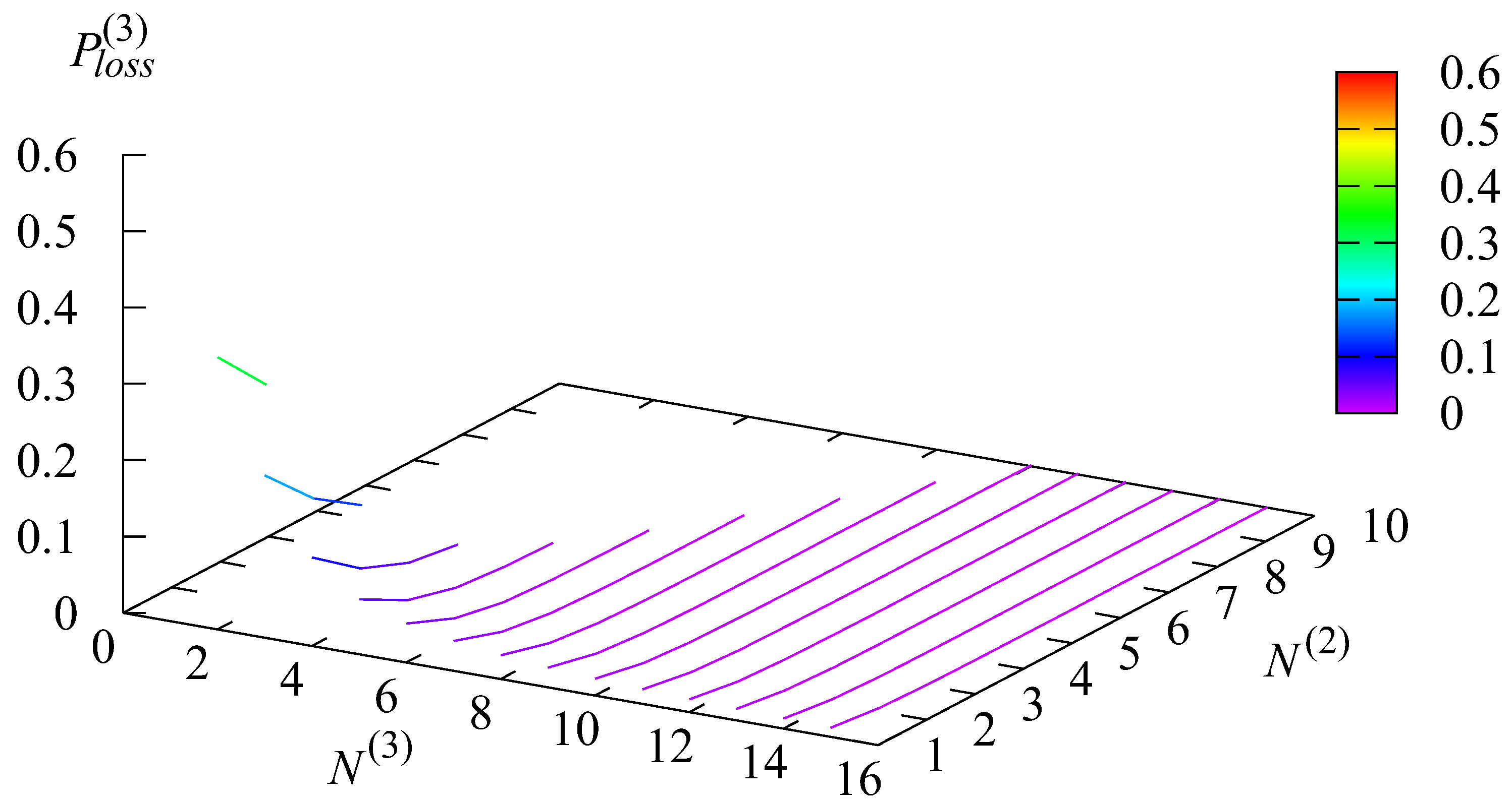
Figure 13,
Figure 14 and
Figure 15 illustrate the dependencies of the loss probability
and the joint loss probabilities
that the
stays in the state
r and a request is lost on the parameters
and
The probability
is the sum of the joint probabilities
Above, we stated that the economical quality of the system’s functioning is mainly defined by the output rate
of the serviced requests. We noted the obvious fact that
increases when the numbers of channels
and
increase. In applications of the considered model, it is necessary to take into account that the purchasing or leasing as well as the maintenance of the channels require expenditures. As a result, the following revenue criterion may be used to assess the system’s operational quality:
where
are the costs for one channel maintained in states 2 and 3 of the
,
b is the fee paid by the system in the event that a request is lost, and
a is the system’s income for one request’s service.
A pair that optimizes the criteria E must be defined. In this numerical example, we set the cost coefficients’ values to the following:
Figure 16 shows the surface that relates the criterion’s dependency on
and
values.
For all values of from 1 to 4, the optimal value of is equal to For from 5 to 15, the optimal value of is equal to 3. The optimal value of the cost criterion E is 2.28548 when and Note that and Thus, the optimal value of the cost criterion is essentially greater than its values in cases where only one channel is exploited in states 2 and 3 of the and when 10 and 15 channels are used, respectively.
Note also that similar optimization problems can be easily solved in more general settings, e.g., when some restrictions on the values of some performance measures, e.g., the mean number of requests in the buffer or the rate of request service termination, are imposed. Such types of problems arise in many real-world service systems, and the outcomes acquired can be used to achieve managerial objectives.
8. Conclusions
In this paper, an type with possible impatient requests is analyzed. An may have an influence on the number of available channels, request arrival and service processes, as well as impatience rates. The results can be useful for a performance analysis of this type of queue under various sets of queue parameters. It is important to remember that occasionally, only a part of the system parameters randomly changes. The other parameters can be varied by a system manager aiming to obtain more revenue or a better service experience. For example, under the known pattern of request arrivals, the service provider can dynamically vary the number of active channels. The number of channels can be increased during periods of peak arrival rates and decreased during periods when the arrival rate is low. Conversely, if the random mechanism of changing the number of channels is known (e.g., if the channels are shared with another service provider and his schedule of channels is known), the service provider can manage the procedures of requests, admitting or rejecting them. Requests can be offered (e.g., via the flexible tariffs) to reduce their arrival rate or service time when the number of channels is small. The findings of the analysis can be useful for optimal decision-making in such and similar situations.
The results can be extended, e.g., to systems with different strategies of admission control and request retrials, systems with heterogeneous requests, priorities, and various channel reservation schemes.


