
A Computational Methodology Based on Maximum Overlap Discrete Wavelet Transform and Autoencoders for Early Prediction of Sudden Cardiac Death

 , ,
, ,  , and
, and 
Abstract
1. Introduction
2. Data and Methods
2.1. ECG Data
2.1.1. Data Used
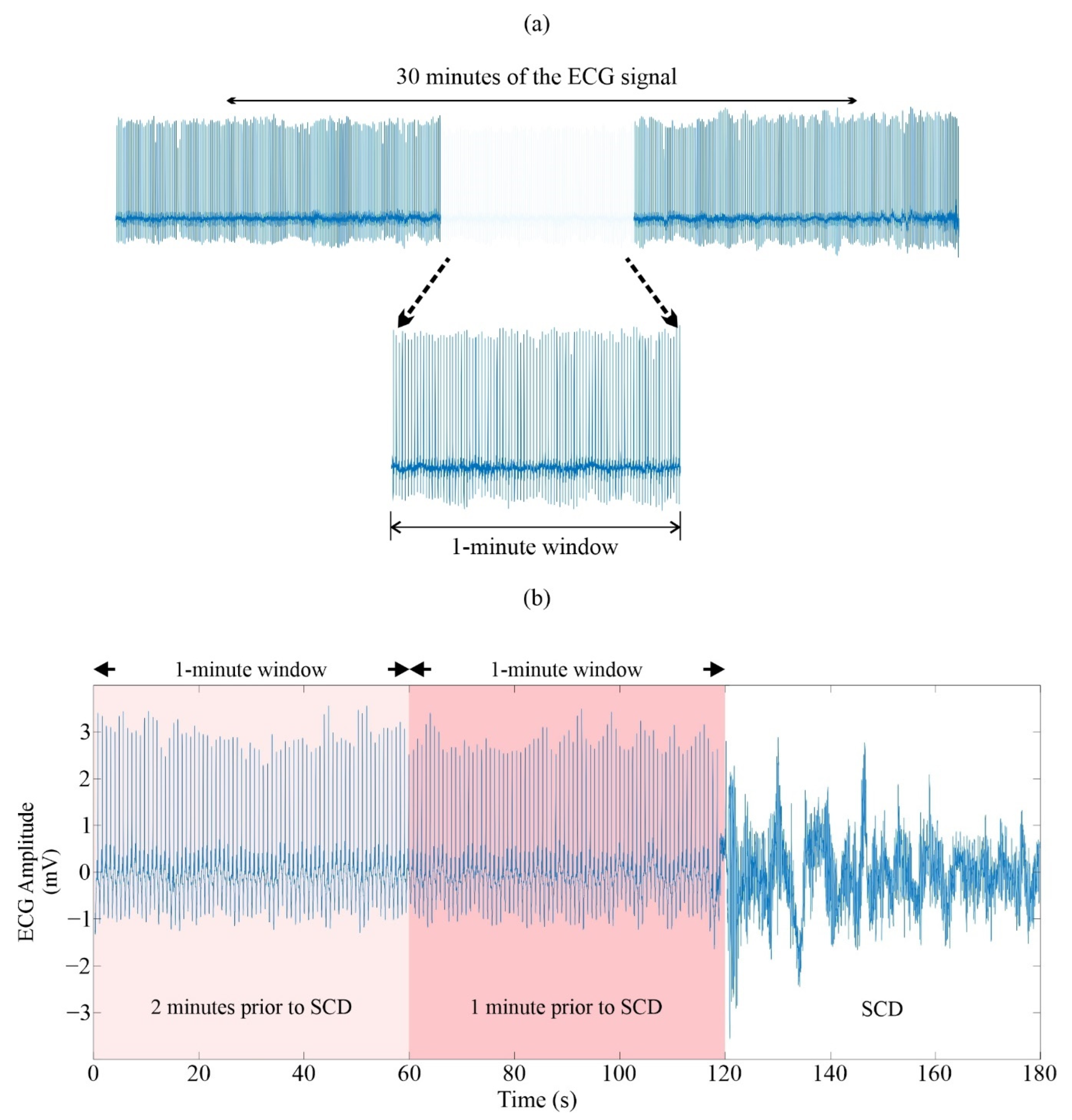
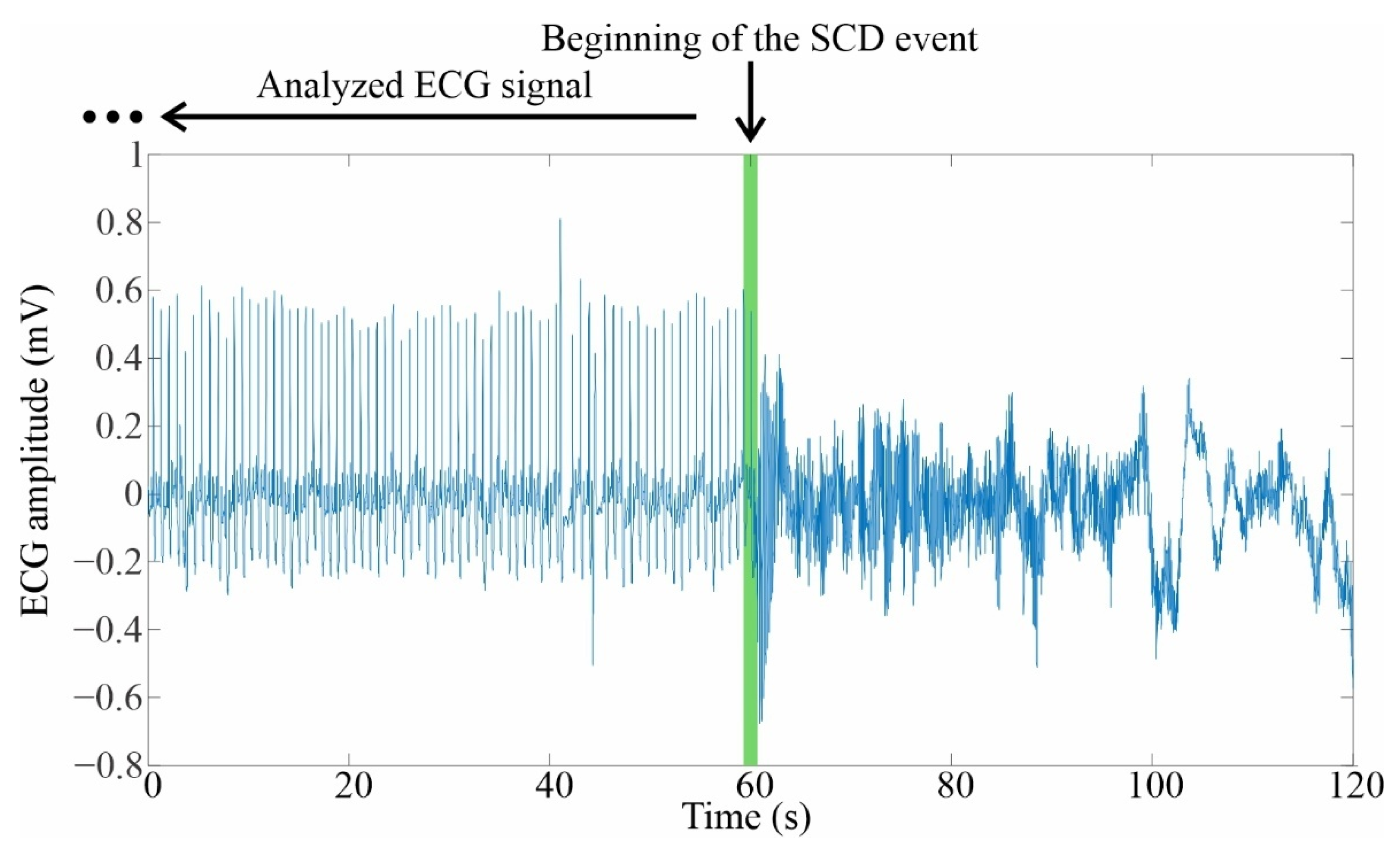
2.1.2. Selection and Preparation of ECG Signals
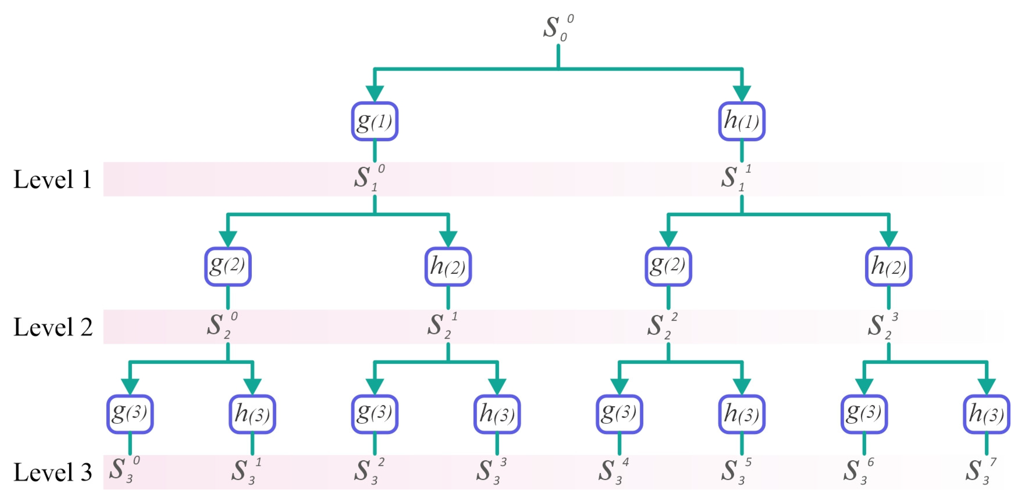
2.2. Maximal Overlapped Discrete Wavelet Packet Transform
2.3. Classifier
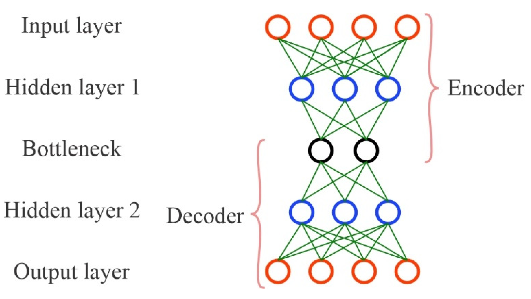
2.3.1. Autoencoder
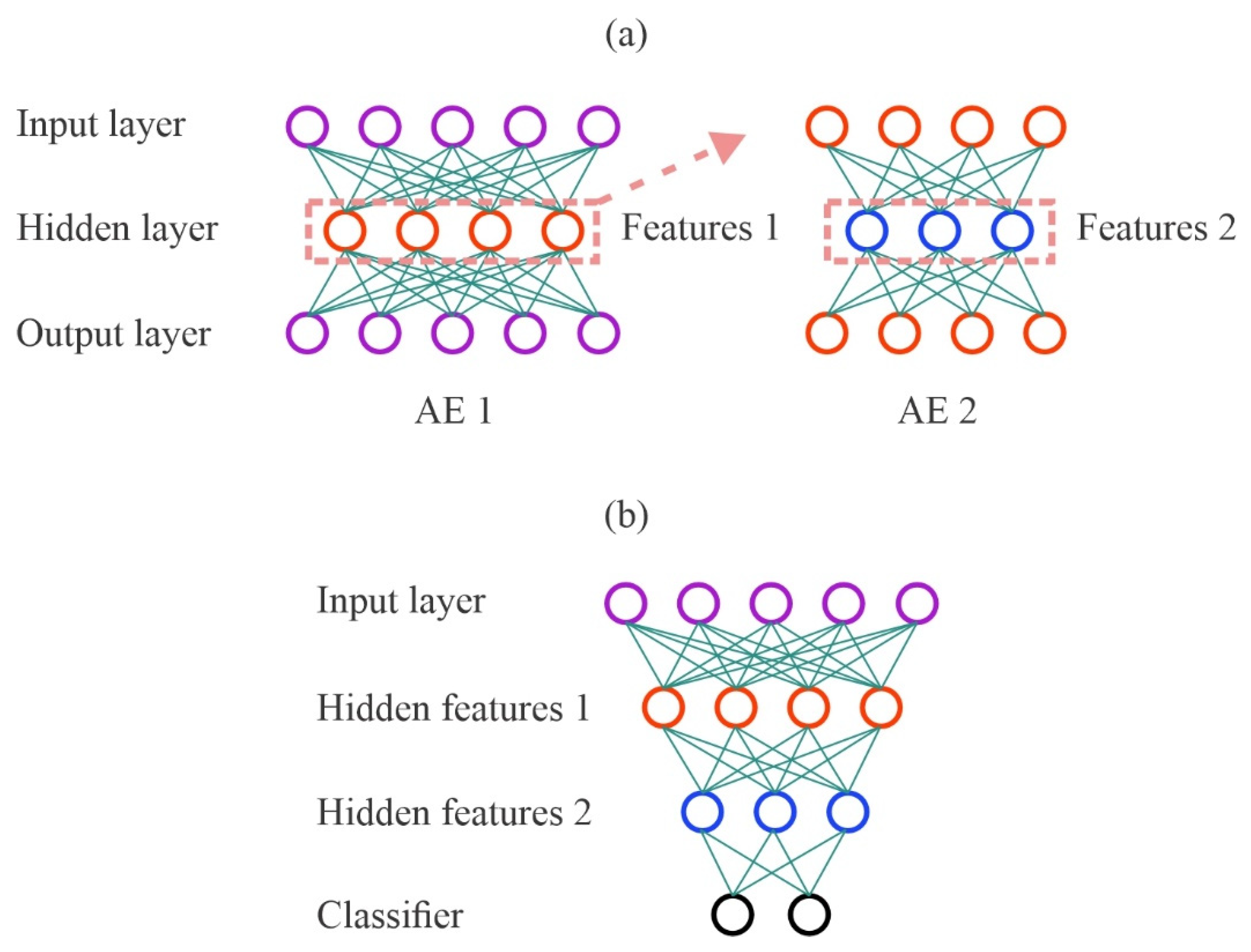
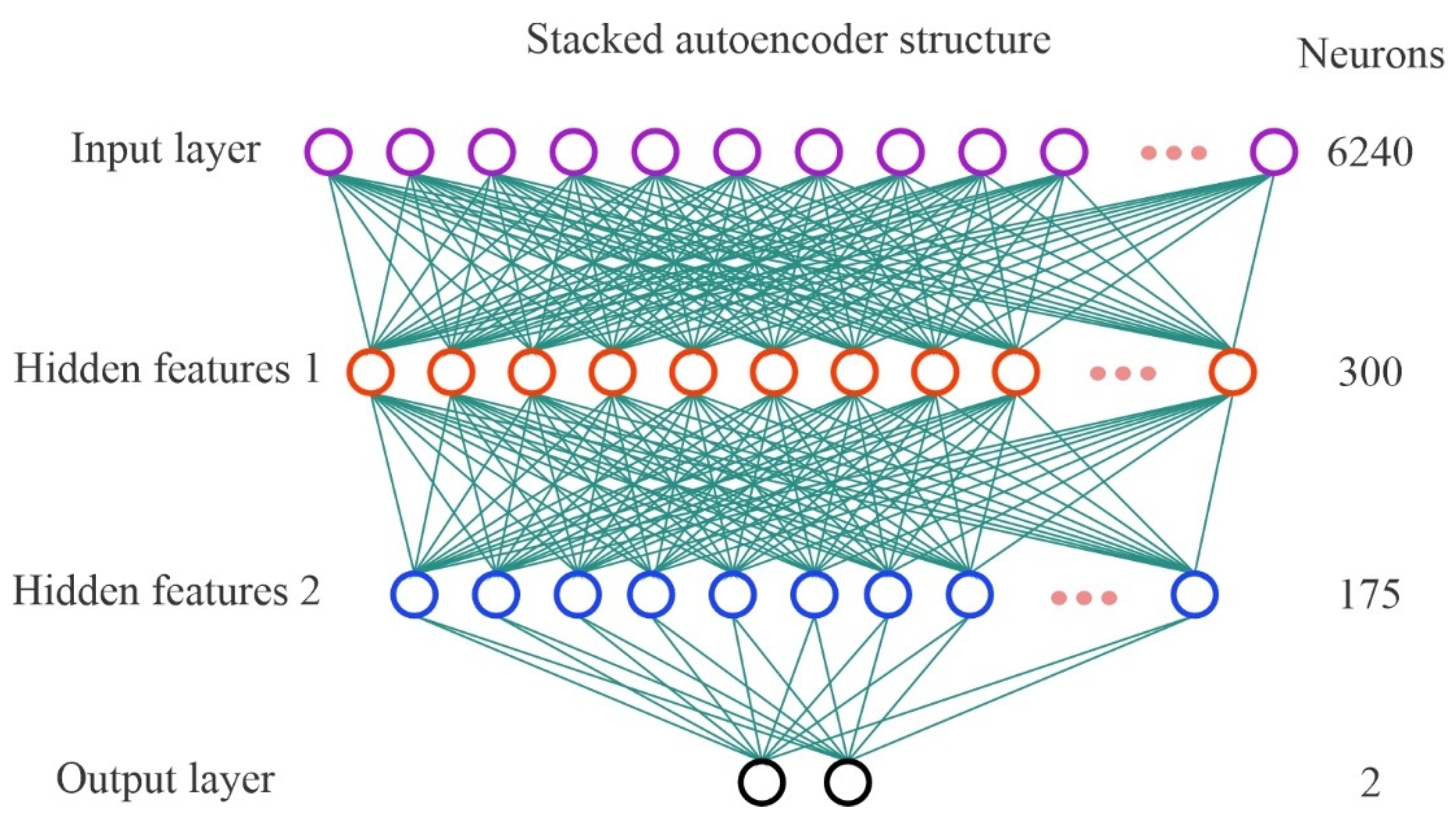
2.3.2. Stacked Autoencoder
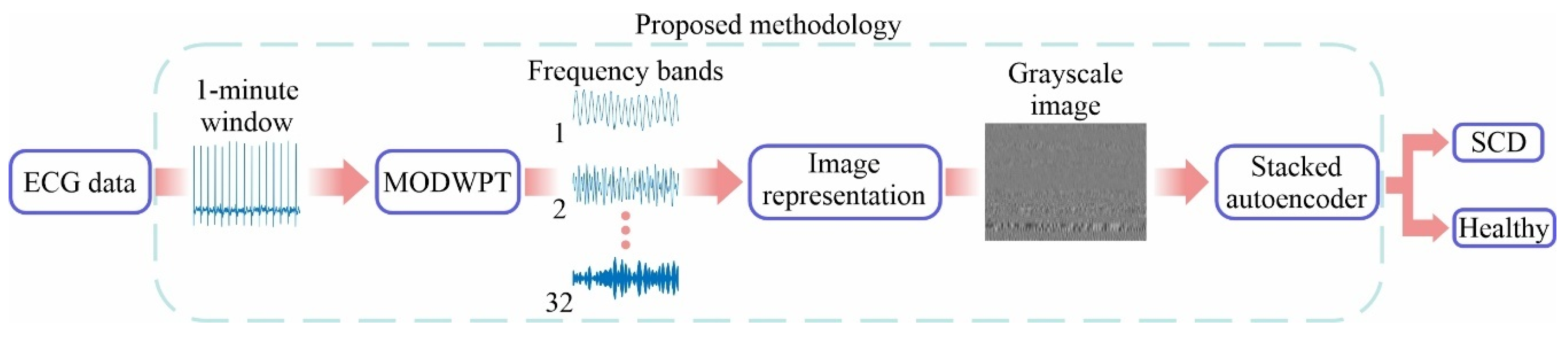
3. Methodology
4. Experimentation and Results
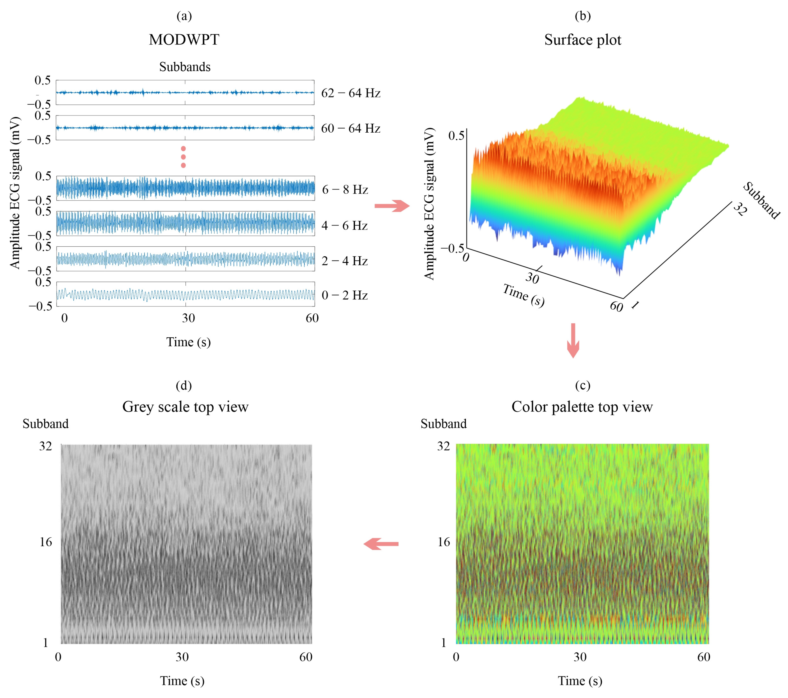
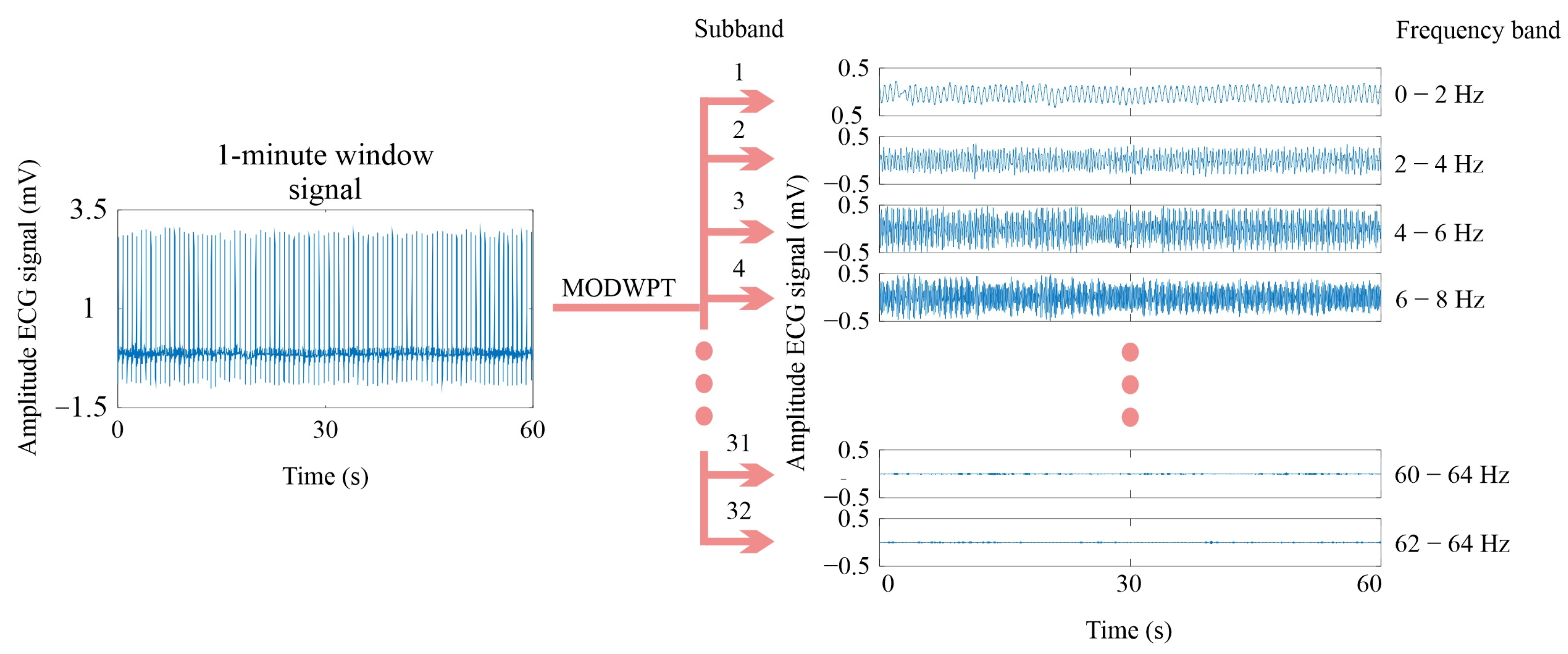
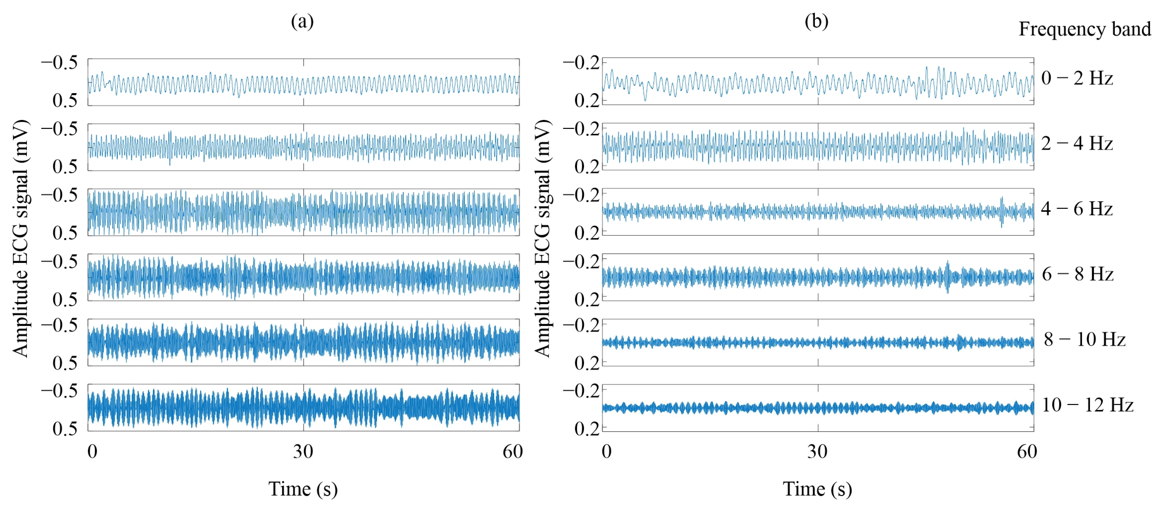
4.1. Signal Decomposition
4.2. Data Classification
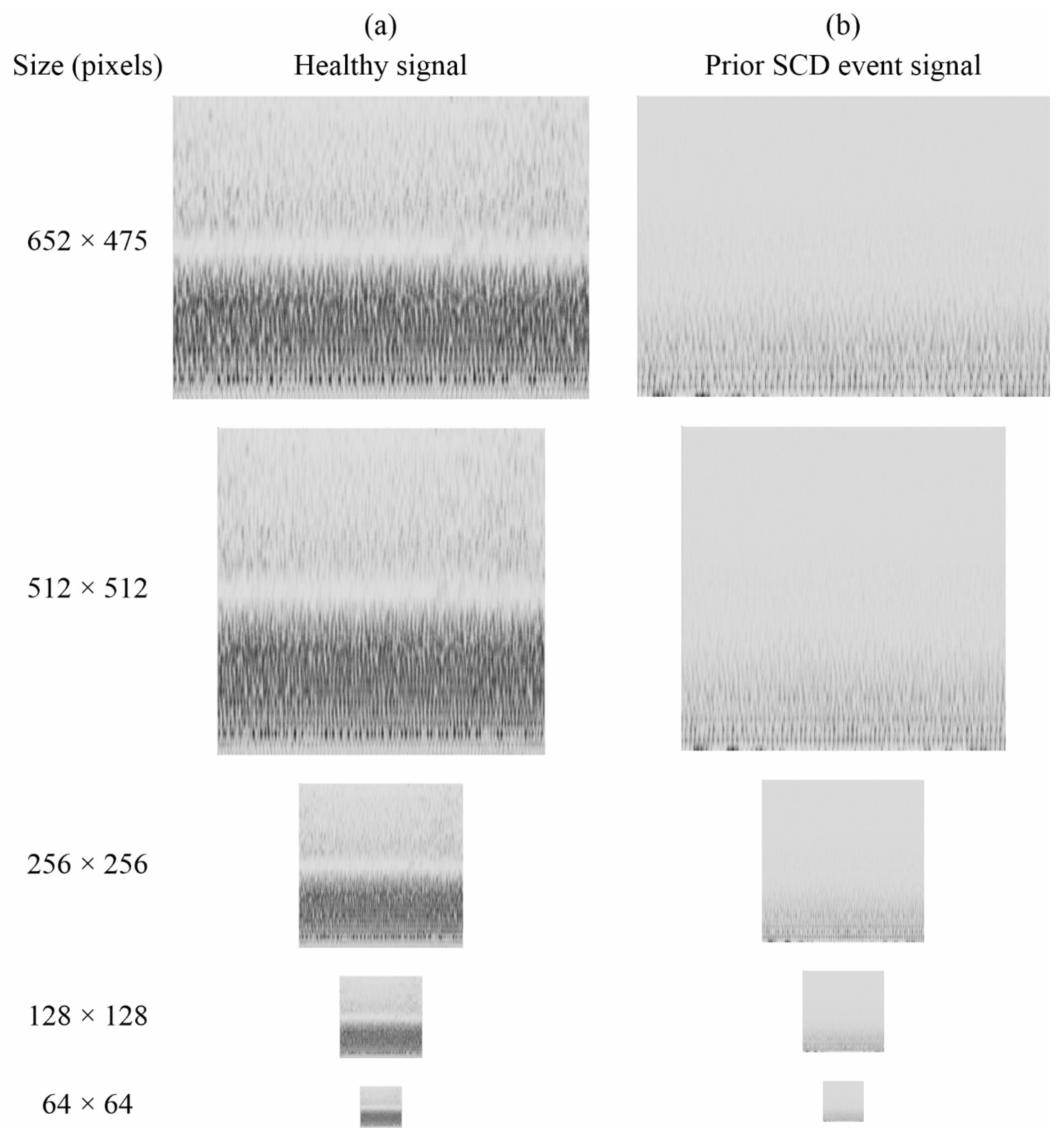
4.2.1. Testing Different Image Sizes
4.2.2. Testing the Number of the Hidden Layer Neurons
5. Discussion
6. Conclusions
Author Contributions
Funding
Institutional Review Board Statement
Informed Consent Statement
Data Availability Statement
Conflicts of Interest
Abbreviations
| AE | Autoencoder |
| CEEMD | Complete Ensemble Empirical Mode |
| CNN | Convolutional Neural Networks |
| DL | Deep Learning |
| DWPT | Discrete Wavelet Packet Transform |
| ECG | Electrocardiogram |
| EMD | Empirical Mode Decomposition |
| FBs | Frequency Bands |
| HHT | Hilbert–Huang Transform |
| LSTM | Long Short-Term Memory Networks |
| ML | Machine Learning |
| MLP | Multilayer Perceptron |
| MODWPT | Maximal Overlap Discrete Wavelet Packet Transform |
| NSR | Normal Sinus Rhythm |
| SAE | Stacked Autoencoders |
| SCD | Sudden Cardiac Death |
| SCDH | Sudden Cardiac Death Holter |
| SVM | Support Vector Machine |
| WPT | Wavelet Packet Transform |
| WT | Wavelet Transform |
References
- Srinivasan, N.T.; Schilling, R.J. Sudden cardiac death and arrhythmias. Arrhythm. Electrophysiol. Rev. 2018, 7, 111–117. [Google Scholar] [CrossRef] [PubMed]
- Paratz, E.D.; Rowsell, L.; Zentner, D.; Parsons, S.; Morgan, N.; Thompson, T.; James, P.; Pflaumer, A.; Semsarian, C.; Smith, K.; et al. Cardiac arrest and sudden cardiac death registries: A systematic review of global coverage. Open Heart 2020, 7, e001195. [Google Scholar] [CrossRef] [PubMed]
- Wong, C.X.; Brown, A.; Lau, D.H.; Chugh, S.S.; Albert, C.M.; Kalman, J.M.; Sanders, P. Epidemiology of Sudden Cardiac Death: Global and Regional Perspectives. Heart Lung Circ. 2019, 28, 6–14. [Google Scholar] [CrossRef]
- Katritsis, D.G.; Gersh, B.J.; Camm, A.J. A clinical perspective on sudden cardiac death. Arrhythm. Electrophysiol. Rev. 2016, 5, 177–182. [Google Scholar] [CrossRef]
- Jazayeri, M.A.; Emert, M.P. Sudden Cardiac Death: Who Is at Risk? Med. Clin. N. Am. 2019, 103, 913–930. [Google Scholar] [CrossRef]
- Myat, A.; Song, K.J.; Rea, T. Out-of-hospital cardiac arrest: Current concepts. Lancet 2018, 391, 970–979. [Google Scholar] [CrossRef]
- Alfarhan, K.A.; Mashor, M.Y.; Zakaria, A.; Omar, M.I. Automated Electrocardiogram Signals Based Risk Marker for Early Sudden Cardiac Death Prediction. J. Med. Imaging Health Inform. 2019, 8, 1769–1775. [Google Scholar] [CrossRef]
- Ebrahimzadeh, E.; Manuchehri, M.S.; Amoozegar, S.; Araabi, B.N.; Soltanian-Zadeh, H. A time local subset feature selection for prediction of sudden cardiac death from ECG signal. Med. Biol. Eng. Comput. 2018, 56, 1253–1270. [Google Scholar] [CrossRef] [PubMed]
- Vargas-Lopez, O.; Amezquita-Sanchez, J.P.; De-Santiago-Perez, J.J.; Rivera-Guillen, J.R.; Valtierra-Rodriguez, M.; Toledano-Ayala, M.; Perez-Ramirez, C.A. A new methodology based on EMD and nonlinear measurements for sudden cardiac death detection. Sensors 2020, 20, 9. [Google Scholar] [CrossRef]
- Ebrahimzadeh, E.; Foroutan, A.; Shams, M.; Baradaran, R.; Rajabion, L.; Joulani, M.; Fayaz, F. An optimal strategy for prediction of sudden cardiac death through a pioneering feature-selection approach from HRV signal. Comput. Methods Programs Biomed. 2019, 169, 19–36. [Google Scholar] [CrossRef]
- Khazaei, M.; Raeisi, K.; Goshvarpour, A.; Ahmadzadeh, M. Early detection of sudden cardiac death using nonlinear analysis of heart rate variability. Biocybern. Biomed. Eng. 2018, 38, 931–940. [Google Scholar] [CrossRef]
- Amezquita-Sanchez, J.P.; Valtierra-Rodriguez, M.; Adeli, H.; Perez-Ramirez, C.A. A Novel Wavelet Transform-Homogeneity Model for Sudden Cardiac Death Prediction Using ECG Signals. J. Med. Syst. 2018, 42, 176. [Google Scholar] [CrossRef] [PubMed]
- Singhal, A.; Agarwal, M. An automatic risk assessment system for sudden cardiac death using look ahead pattern. Multimed. Tools Appl. 2024, 83, 27243–27258. [Google Scholar] [CrossRef]
- Centeno-Bautista, M.A.; Perez-Sanchez, A.V.; Amezquita-Sanchez, J.P.; Valtierra-Rodriguez, M. Sudden cardiac death prediction based on the complete ensemble empirical mode decomposition method and a machine learning strategy by using ECG signals. Measurement 2024, 236, 115052. [Google Scholar] [CrossRef]
- Trayanova, N.A.; Topol, E.J. Deep learning a person’s risk of sudden cardiac death. Lancet 2022, 399, 1933. [Google Scholar] [CrossRef]
- Barker, J.; Li, X.; Khavandi, S.; Koeckerling, D.; Mavilakandy, A.; Pepper, C.; Bountziouka, V.; Chen, L.; Kotb, A.; Antoun, I.; et al. Machine learning in sudden cardiac death risk prediction: A systematic review. Europace 2022, 24, 1777–1787. [Google Scholar] [CrossRef]
- Eleyan, A.; Alboghbaish, E. Electrocardiogram Signals Classification Using Deep-Learning-Based Incorporated Convolutional Neural Network and Long Short-Term Memory Framework. Computers 2024, 13, 55. [Google Scholar] [CrossRef]
- Seitanidis, P.; Gialelis, J.; Papaconstantinou, G.; Moschovas, A. Identification of Heart Arrhythmias by Utilizing a Deep Learning Approach of the ECG Signals on Edge Devices. Computers 2022, 11, 176. [Google Scholar] [CrossRef]
- Acharya, U.R.; Fujita, H.; Oh, S.L.; Hagiwara, Y.; Tan, J.H.; Adam, M. Application of deep convolutional neural network for automated detection of myocardial infarction using ECG signals. Inf. Sci. 2017, 415–416, 190–198. [Google Scholar] [CrossRef]
- Shilla, W.; Wang, X. Wavelet Transform and Convolutional Neural Network Based Techniques in Combating Sudden Cardiac Death. EMITTER Int. J. Eng. Technol. 2021, 9, 377–389. [Google Scholar] [CrossRef]
- Kwon, J.M.; Kim, K.H.; Jeon, K.H.; Park, J. Deep learning for predicting in-hospital mortality among heart disease patients based on echocardiography. Echocardiography 2019, 36, 213–218. [Google Scholar] [CrossRef] [PubMed]
- Kwon, J.M.; Lee, Y.; Lee, Y.; Lee, S.; Park, J. An algorithm based on deep learning for predicting in-hospital cardiac arrest. J. Am. Heart Assoc. 2018, 7, 13. [Google Scholar] [CrossRef]
- Saragih, Y.V.; Isa, S.M. CNN performance improvement using wavelet packet transform for sca prediction. J. Theor. Appl. Inf. Technol. 2022, 100, 5458–5468. [Google Scholar]
- Kaspal, R.; Alsadoon, A.; Prasad, P.W.C.; Al-Saiyd, N.A.; Nguyen, T.Q.V.; Pham, D.T.H. A novel approach for early prediction of sudden cardiac death (SCD) using hybrid deep learning. Multimed. Tools Appl. 2021, 80, 8063–8090. [Google Scholar] [CrossRef]
- Telangore, H.; Azad, V.; Sharma, M.; Bhurane, A.; Tan, R.S.; Acharya, U.R. Early prediction of sudden cardiac death using multimodal fusion of ECG Features extracted from Hilbert–Huang and wavelet transforms with explainable vision transformer and CNN models. Comput. Methods Programs Biomed. 2024, 257, 108455. [Google Scholar] [CrossRef] [PubMed]
- Centeno-Bautista, M.A.; Rangel-Rodriguez, A.H.; Perez-Sanchez, A.V.; Amezquita-Sanchez, J.P.; Granados-Lieberman, D.; Valtierra-Rodriguez, M. Electrocardiogram Analysis by Means of Empirical Mode Decomposition-Based Methods and Convolutional Neural Networks for Sudden Cardiac Death Detection. Appl. Sci. 2023, 13, 3569. [Google Scholar] [CrossRef]
- Alves, D.K.; Costa, F.B.; Ribeiro, R.L.D.A.; Sousa Neto, C.M.D.; Rocha, T.D.O.A. Real-time power measurement using the maximal overlap discrete wavelet-packet transform. IEEE Trans. Ind. Electron. 2017, 64, 3177–3187. [Google Scholar] [CrossRef]
- Yang, D.M. The detection of motor bearing fault with maximal overlap discrete wavelet packet transform and teager energy adaptive spectral kurtosis. Sensors 2021, 21, 6895. [Google Scholar] [CrossRef]
- Zhang, T.; Chen, W.; Li, M. Classification of inter-ictal and ictal EEGs using multi-basis MODWPT, dimensionality reduction algorithms and LS-SVM: A comparative study. Biomed. Signal Process. Control 2019, 47, 240–251. [Google Scholar] [CrossRef]
- Han, C.; Shi, L. Automated interpretable detection of myocardial infarction fusing energy entropy and morphological features. Comput. Methods Programs Biomed. 2019, 175, 9–23. [Google Scholar] [CrossRef]
- Al-Naami, B.; Fraihat, H.; Owida, H.A.; Al-Hamad, K.; De Fazio, R.; Visconti, P. Automated Detection of Left Bundle Branch Block from ECG Signal Utilizing the Maximal Overlap Discrete Wavelet Transform with ANFIS. Computers 2022, 11, 93. [Google Scholar] [CrossRef]
- Perez-Sanchez, A.V.; Amezquita-Sanchez, J.P.; Valtierra-Rodriguez, M.; Adeli, H. A new epileptic seizure prediction model based on maximal overlap discrete wavelet packet transform, homogeneity index, and machine learning using ECG signals. Biomed. Signal Process. Control 2024, 88, 105659. [Google Scholar] [CrossRef]
- Balasubaramanian, S.; Cyriac, R.; Roshan, S.; Maruthamuthu Paramasivam, K.; Chellanthara Jose, B. An effective stacked autoencoder based depth separable convolutional neural network model for face mask detection. Array 2023, 19, 100294. [Google Scholar] [CrossRef] [PubMed]
- Soleymani, F.; Paquet, E. Financial portfolio optimization with online deep reinforcement learning and restricted stacked autoencoder—DeepBreath. Expert Syst. Appl. 2020, 156, 113456. [Google Scholar] [CrossRef]
- Wang, L.; You, Z.H.; Chen, X.; Xia, S.X.; Liu, F.; Yan, X.; Zhou, Y.; Song, K.J. A computational-based method for predicting drug-target interactions by using stacked autoencoder deep neural network. J. Comput. Biol. 2018, 25, 361–373. [Google Scholar] [CrossRef]
- Idowu, O.P.; Ilesanmi, A.E.; Li, X.; Samuel, O.W.; Fang, P.; Li, G. An integrated deep learning model for motor intention recognition of multi-class EEG Signals in upper limb amputees. Comput. Methods Programs Biomed. 2021, 206, 106121. [Google Scholar] [CrossRef]
- Yin, Z.; Zhao, M.; Wang, Y.; Yang, J.; Zhang, J. Recognition of emotions using multimodal physiological signals and an ensemble deep learning model. Comput. Methods Programs Biomed. 2017, 140, 93–110. [Google Scholar] [CrossRef]
- Goldberger, A.L.; Amaral, L.A.N.; Glass, L.; Hausdorff, J.M.; Ivanov, P.C.; Mark, R.G.; Mietus, J.E.; Moody, G.B.; Peng, C.-K.; Stanley, H.E. PhysioBank, PhysioToolkit, and PhysioNet. Circulation 2000, 101, E215–E220. [Google Scholar] [CrossRef] [PubMed]
- Chinara, S. Automatic classification methods for detecting drowsiness using wavelet packet transform extracted time-domain features from single-channel EEG signal. J. Neurosci. Methods 2021, 347, 108927. [Google Scholar] [CrossRef]
- Shrifan, N.H.M.M.; Akbar, M.F.; Mat Isa, N.A. Maximal overlap discrete wavelet-packet transform aided microwave non-destructive testing. NDT E Int. 2021, 119, 102414. [Google Scholar] [CrossRef]
- Dai, X.; Cheng, J.; Guo, S.; Wang, C.; Qu, G.; Liu, W.; Li, W.; Lu, H.; Wang, Y.; Zeng, B.; et al. Optimization Strategy of a Stacked Autoencoder and Deep Belief Network in a Hyperspectral Remote-Sensing Image Classification Model. Discret. Dyn. Nat. Soc. 2023, 2023, 9150482. [Google Scholar] [CrossRef]
- Bai, Y.; Sun, X.; Ji, Y.; Fu, W.; Zhang, J. Two-stage multi-dimensional convolutional stacked autoencoder network model for hyperspectral images classification. Multimed. Tools Appl. 2024, 83, 23489–23508. [Google Scholar] [CrossRef]
- Rafiee, J.; Rafiee, M.A.; Prause, N.; Schoen, M.P. Wavelet basis functions in biomedical signal processing. Expert Syst. Appl. 2011, 38, 6190–6201. [Google Scholar] [CrossRef]
- Dong, G.; Liao, G.; Liu, H.; Kuang, G. A Review of the Autoencoder and Its Variants: A Comparative Perspective from Target Recognition in Synthetic-Aperture Radar Images. IEEE Geosci. Remote Sens. Mag. 2018, 6, 44–68. [Google Scholar] [CrossRef]
- Yang, Z.; Xu, B.; Luo, W.; Chen, F. Autoencoder-based representation learning and its application in intelligent fault diag-nosis: A review. Measurement 2022, 189, 110460. [Google Scholar] [CrossRef]
- Gadhiya, T.; Tangirala, S.; Roy, A.K. Stacked Autoencoder Based Feature Extraction and Superpixel Generation for Mul-tifrequency PolSAR Image Classification. In Lecture Notes in Computer Science (Including Subseries Lecture Notes in Artificial Intelligence and Lecture Notes in Bioinformatics); Springer: Berlin/Heidelberg, Germany, 2019; pp. 331–339. [Google Scholar] [CrossRef]
- Liu, S.; Zhang, C.; Ma, J. Stacked auto-encoders for feature extraction with neural networks. In Communications in Computer and Information Science; Springer: Berlin/Heidelberg, Germany, 2016; pp. 377–384. [Google Scholar] [CrossRef]
- Li, D.; Fu, Z.; Xu, J. Stacked-autoencoder-based model for COVID-19 diagnosis on CT images. Appl. Intell. 2002, 51, 2805–2817. [Google Scholar] [CrossRef]
- Zhou, P.; Han, J.; Cheng, G.; Zhang, B. Learning Compact and Discriminative Stacked Autoencoder for Hyperspectral Im-age Classification. IEEE Trans. Geosci. Remote Sens. 2019, 57, 4823–4833. [Google Scholar] [CrossRef]
- Vareka, L.; Mautner, P. Stacked autoencoders for the P300 component detection. Front. Neurosci. 2017, 11, 302. [Google Scholar] [CrossRef] [PubMed]
- Willigenburg, N.W.; Daffertshofer, A.; Kingma, I.; van Dieën, J.H. Removing ECG contamination from EMG recordings: A comparison of ICA-based and other filtering procedures. J. Electromyogr. Kinesiol. 2012, 22, 485–493. [Google Scholar] [CrossRef]
- Walden, A.T.; Contreras Cristan, A. The Phase-Corrected Undecimated Discrete Wavelet Packet Transform and Its Application to Interpreting the Timing of Events. Available online: https://royalsocietypublishing.org/ (accessed on 24 April 2025).
- Hagara, M.; Stojanović, R.; Bagala, T.; Kubinec, P.; Ondráček, O. Grayscale image formats for edge detection and for its FPGA implementation. Microprocess. Microsyst. 2020, 75, 103056. [Google Scholar] [CrossRef]
- Dhanya, L.; Chitra, R. A novel autoencoder based feature independent GA optimised XGBoost classifier for IoMT mal-ware detection. Expert Syst. Appl. 2024, 237, 121618. [Google Scholar] [CrossRef]
- Singh, J.P.; Kumar, M. Chaotic whale-atom search optimization-based deep stacked auto encoder for crowd behaviour recognition. J. Exp. Theor. Artif. Intell. 2024, 36, 187–211. [Google Scholar] [CrossRef]
- Alwahedi, F.; Aldhaheri, A.; Ferrag, M.A.; Battah, A.; Tihanyi, N. Machine learning techniques for IoT security: Current research and future vision with generative AI and large language models. Internet Things Cyber-Phys. Syst. 2024, 4, 167–185. [Google Scholar] [CrossRef]

| Image Size (Pixels) | Average Accuracy (%) |
|---|---|
| 652 × 475 | 96.04 |
| 512 × 512 | 95.17 |
| 256 × 256 | 95.70 |
| 128 × 128 | 98.15 |
| 64 × 64 | 96.14 |
| First AE Hidden Layer Neurons | Average Accuracy (%) |
|---|---|
| 400 | 97.89 |
| 300 | 98.68 |
| 200 | 98.15 |
| 100 | 94.91 |
| 75 | 91.40 |
| Second AE Hidden Layer Neurons | Average Accuracy (%) |
|---|---|
| 200 | 98.85 |
| 175 | 98.94 |
| 150 | 98.85 |
| 125 | 98.68 |
| 100 | 98.68 |
| 75 | 96.68 |
| 50 | 98.68 |
| 25 | 98.5 |
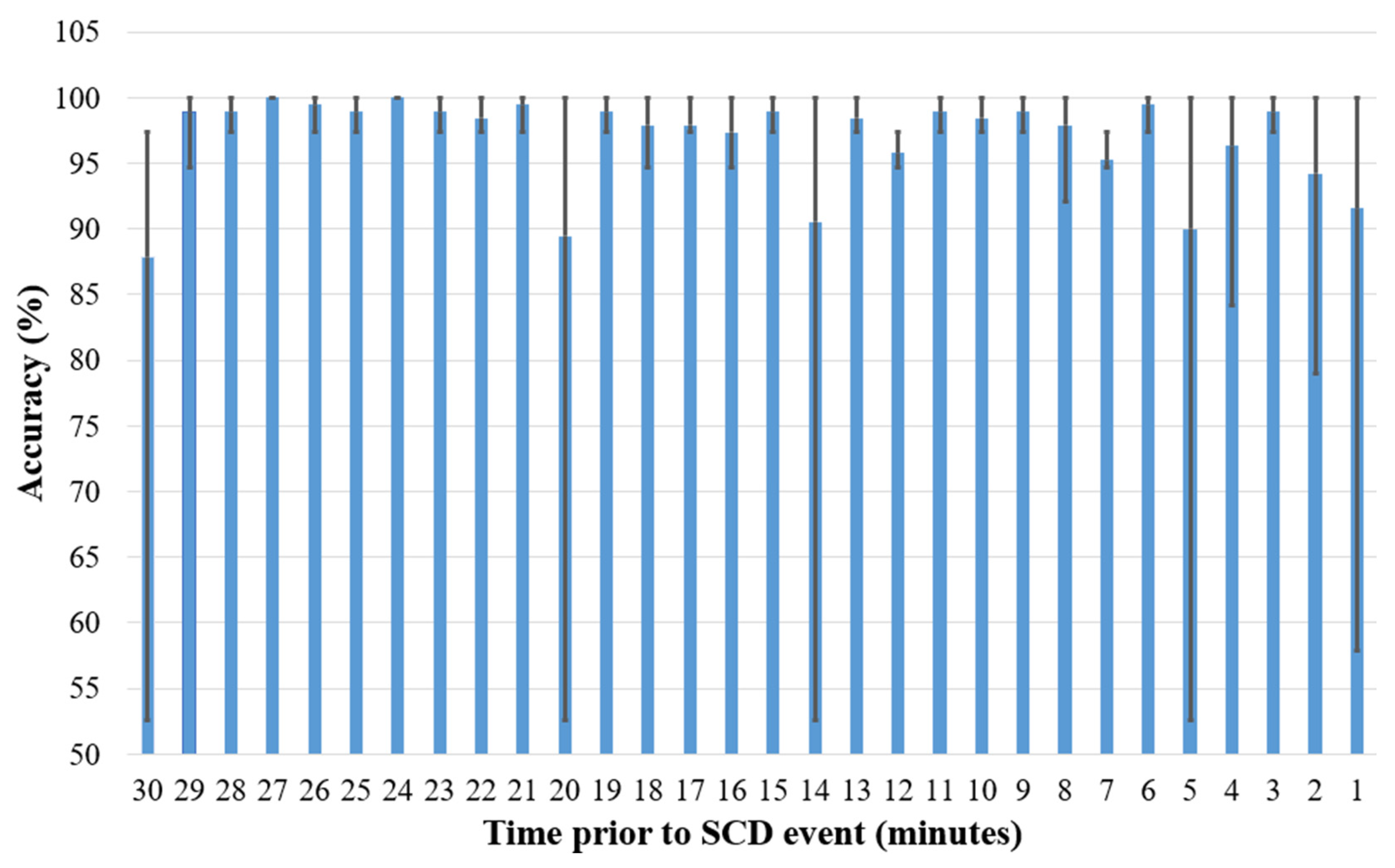
| Minutes Prior to SCD Event | Accuracy (%) | Minutes Prior to SCD Event | Accuracy (%) |
|---|---|---|---|
| 1 | 100 | 16 | 100 |
| 2 | 100 | 17 | 100 |
| 3 | 100 | 18 | 97.36 |
| 4 | 97.36 | 19 | 100 |
| 5 | 100 | 20 | 100 |
| 6 | 97.36 | 21 | 97.36 |
| 7 | 97.36 | 22 | 97.36 |
| 8 | 100 | 23 | 100 |
| 9 | 100 | 24 | 100 |
| 10 | 97.36 | 25 | 100 |
| 11 | 97.36 | 26 | 100 |
| 12 | 97.36 | 27 | 100 |
| 13 | 97.36 | 28 | 97.36 |
| 14 | 100 | 29 | 100 |
| 15 | 100 | 30 | 97.36 |
| Work | Data Processing | Classifier | Accuracy/Prediction Time |
|---|---|---|---|
| Alfarhan et al. [7] | Mean, standard deviation | K-nearest neighbor | 97%/10 min |
| Ebrahimzadeh et al. [8] | First derivative feature | MLP | 83%/12 min |
| Vargas-Lopez et al. [9] | EMD, Higuchi fractal | MLP | 94%/24 min |
| Ebrahimzadeh et al. [10] | Standard deviation from variability heart rate | MLP | 90.18%/13 min |
| Khazaei et al. [11] | Recurrence quantification analysis | Decision tree | 95%/6 min |
| Amezquita-Sanchez et al. [12] | WPT, homogeneity index | Probabilistic neural network | 95.8%/20 min |
| Singhal and Agarwal [13] | Fourier-based decomposition technique | min | 100%/10 min |
| Centeno-Bautista et al. [14] | CEEMD | SVM | 97.28%/30 min |
| Saraghi and Isa [23] | WPT | CNN | 95.89%/30 min |
| Kaspal et al. [24] | Recurrence complex network | CNN | 90.6%/30 min |
| Telangore et al. [25] | HHT, WT | CNN | 98.81%/30 min |
| Centeno-Bautista et al. [26] | CEEMD | CNN | 97.5%/30 min |
| Proposed work | MODWPT | Stacked autoencoders | 98.94%/30 min |
Disclaimer/Publisher’s Note: The statements, opinions and data contained in all publications are solely those of the individual author(s) and contributor(s) and not of MDPI and/or the editor(s). MDPI and/or the editor(s) disclaim responsibility for any injury to people or property resulting from any ideas, methods, instructions or products referred to in the content. |
© 2025 by the authors. Licensee MDPI, Basel, Switzerland. This article is an open access article distributed under the terms and conditions of the Creative Commons Attribution (CC BY) license (https://creativecommons.org/licenses/by/4.0/).
Share and Cite
Centeno-Bautista, M.A.; Perez-Sanchez, A.V.; Amezquita-Sanchez, J.P.; Camarena-Martinez, D.; Valtierra-Rodriguez, M. A Computational Methodology Based on Maximum Overlap Discrete Wavelet Transform and Autoencoders for Early Prediction of Sudden Cardiac Death. Computation 2025, 13, 130. https://doi.org/10.3390/computation13060130
Centeno-Bautista MA, Perez-Sanchez AV, Amezquita-Sanchez JP, Camarena-Martinez D, Valtierra-Rodriguez M. A Computational Methodology Based on Maximum Overlap Discrete Wavelet Transform and Autoencoders for Early Prediction of Sudden Cardiac Death. Computation. 2025; 13(6):130. https://doi.org/10.3390/computation13060130
Chicago/Turabian StyleCenteno-Bautista, Manuel A., Andrea V. Perez-Sanchez, Juan P. Amezquita-Sanchez, David Camarena-Martinez, and Martin Valtierra-Rodriguez. 2025. "A Computational Methodology Based on Maximum Overlap Discrete Wavelet Transform and Autoencoders for Early Prediction of Sudden Cardiac Death" Computation 13, no. 6: 130. https://doi.org/10.3390/computation13060130
APA StyleCenteno-Bautista, M. A., Perez-Sanchez, A. V., Amezquita-Sanchez, J. P., Camarena-Martinez, D., & Valtierra-Rodriguez, M. (2025). A Computational Methodology Based on Maximum Overlap Discrete Wavelet Transform and Autoencoders for Early Prediction of Sudden Cardiac Death. Computation, 13(6), 130. https://doi.org/10.3390/computation13060130