Abstract
Addressing unemployment is essential for formulating effective public policies. In particular, socioeconomic and monetary variables serve as essential indicators for anticipating labor market trends, given their strong influence on employment dynamics and economic stability. However, effective unemployment rate prediction requires addressing the non-stationary and non-linear characteristics of labor data. Equally important is the preservation of interpretability in both samples and features to ensure that forecasts can meaningfully inform public decision-making. Here, we provide an explainable framework integrating unsupervised and supervised machine learning to enhance unemployment rate prediction and interpretability. Our approach is threefold: (i) we gather a dataset for Colombian unemployment rate prediction including monetary and socioeconomic variables. (ii) Then, we used a Local Biplot technique from the widely recognized Uniform Manifold Approximation and Projection (UMAP) method along with local affine transformations as an unsupervised representation of non-stationary and non-linear data patterns in a simplified and comprehensible manner. (iii) A Gaussian Processes regressor with kernel-based feature relevance analysis is coupled as a supervised counterpart for both unemployment rate prediction and input feature importance analysis. We demonstrated the effectiveness of our proposed approach through a series of experiments conducted on our customized database focused on unemployment indicators in Colombia. Furthermore, we carried out a comparative analysis between traditional statistical techniques and modern machine learning methods. The results revealed that our framework significantly enhances both clustering and predictive performance, while also emphasizing the importance of input samples and feature selection in driving accurate outcomes.
1. Introduction
Unemployment persists as a deep-rooted structural challenge in economies worldwide, with its impact especially acute in emerging markets [1]. From a macroeconomic perspective, elevated unemployment rates lead to substantial production losses, often reflected in a negative output gap—where actual output lags behind potential, even amid periods of economic growth [2]. This persistent underutilization of resources can trigger a cycle of economic contraction, leading to deeper recessions and potentially prolonged depressions, especially in vulnerable emerging economies [3]. Furthermore, rising unemployment exacerbates socio-economic challenges by diminishing both individual and collective incomes, thereby escalating poverty rates and worsening financial inequality [4]. For instance, in response to the unfavorable economic climate of 2023, central banks worldwide implemented aggressive monetary policies, marking the most rapid escalation of intervention interest rates since the 1980s [5].
Specifically for Colombia, the unemployment rate has reached alarming levels, peaking at a historical high of 26% during the 1999 financial crisis and remaining elevated at 13.25% throughout 2023. This contrasts sharply with the global unemployment rate, which was 5.1% in 2023, revealing a stark employment dissatisfaction gap that affected nearly 435 million people worldwide [6]. Despite numerous policy initiatives, Colombia’s unemployment rate has consistently remained near 10%, underscoring the limited effectiveness of existing employment generation strategies in fostering meaningful improvements in national labor market outcomes. This sustained high level of unemployment points to deeper structural deficiencies, where prevailing policies have failed to disrupt the cycle of joblessness. As a result, a substantial segment of the population continues to be excluded from formal labor market participation, reinforcing patterns of economic marginalization and social inequality [7].
Hence, accurately predicting unemployment rates is essential for governments to formulate effective policies that enhance well-being and foster sustainable development. Precise forecasts enable policymakers to foresee economic difficulties and formulate ways to alleviate the detrimental impacts on society and economy [8]. Such information is especially critical in countries characterized by diverse and rapidly changing socio-economic conditions, i.e., Colombia, where reliable forecasting plays a central role in shaping responsive and effective policy interventions [9]. The success of these policies is intrinsically linked to the accuracy of unemployment projections, as robust forecasts enable more informed decision-making and efficient allocation of public resources [10]. Therefore, enhancing the precision of unemployment forecasting is not merely a technical endeavor but a strategic imperative for sound economic planning and policy design [11].
Nevertheless, accurate unemployment forecasting necessitates the integration of both monetary and socioeconomic variables, as these indicators capture key labor market dynamics and the broader impact of economic policies [12]. Moreover, incorporating data from multiple, heterogeneous sources is essential, as it provides critical insights into economic activity, inflation, interest rates, and employment conditions. To ensure the robustness and reliability of predictive models, it is also vital to harmonize data both spatially and temporally—aligning measurements across consistent geographic regions and timeframes to preserve coherence and comparability [13]. The quality and accessibility of these data sources are pivotal for building comprehensive and representative datasets to support the development of more targeted and effective policy responses [14].
In Colombia, the Departamento Administrativo Nacional de Estadística (DANE) produces official labor market statistics using methodologies aligned with international standards, thereby ensuring consistency and cross-national comparability [15]. However, the absence of binding regulations mandating the synchronization of statistical data across governmental entities poses a risk to the reliability and coherence of unemployment rate predictive models. As the principal authority of the Sistema Estadístico Nacional (SEN), DANE is entrusted with coordinating, regulating, and modernizing national statistical processes. While it holds the mandate to oversee data review and methodological updates, the lack of explicit institutional requirements for inter-agency data harmonization continues to hinder the consistency and integration of labor market information [16].
On the other hand, unemployment forecasting is inherently challenged by the non-stationary and non-linear nature of economic data [17,18]. Non-stationarity implies that key statistical properties—such as the mean and variance of the unemployment rate—vary over time, making it difficult to develop stable and consistently reliable predictive models [19]. As a result, forecasting models may perform well during certain periods but lose accuracy under different economic conditions [20]. Additionally, the presence of linear and non-linear data behaviors indicates that the relationships between unemployment and its driving factors are not fixed, but instead adapt over time in response to shifting macroeconomic conditions [21,22]. This complexity underscores the need for adaptive and explainable modeling approaches that can capture such temporal and structural variations. Therefore, comprehending and surmounting these obstacles is crucial for formulating effective policies intended to decrease unemployment and mitigate its socio-economic effects [23].
In economic science, classical statistical methods for unemployment prediction primarily involve time series models and econometric techniques that have been fundamental in economic forecasting [24]. Traditional approaches, such as the Autoregressive Integrated Moving Average (ARIMA) and its variants, have been widely used to predict unemployment data due to their ability to capture trends and seasonality [25]. Likewise, Vector Autoregression (VAR) and structural equation models provide insights into the relationships between unemployment and macroeconomic variables [26]. Despite their widespread use, these techniques often face limitations in handling the non-stationarity and non-linearity issues [27]. Then, recent advancements have focused on improving these classical models by incorporating techniques such as unit root tests to assess stationary and co-integration strategies to explore long-term equilibrium relationships [28]. While these algorithms remain valuable for their interpretability and simplicity, they are increasingly being integrated with modern computational techniques to enhance predictive performance in complex economic environments.
The increasing demand to simulate intricate and dynamic economic phenomena has hastened the implementation of machine learning methodologies for predictive endeavors [29]. These methodologies have demonstrated significant efficacy in identifying non-linear correlations, accommodating structural shifts in labor markets, and improving forecasting accuracy across various geographies and temporal spans [30]. Furthermore, incorporating various economic indicators into machine learning frameworks has enhanced the capacity to discern causal links and augment the interpretability of predictions [31]. Therefore, Support Vector Machines (SVM), Random Forest (RF), and Gaussian Processes (GP), have been extensively utilized in predictive modeling due to their solid theoretical foundations and adaptability to diverse data structures [32]. SVMs determine an optimal hyperplane in a reproducing kernel Hilbert space; however, their effectiveness may decline with large datasets due to increased computational complexity and sensitivity to kernel hyperparameter selection [33]. Furthermore, RF, as an ensemble method that mitigates overfitting through the aggregation of multiple decision trees, enhances both robustness and interpretability [34]. However, its efficacy often diminishes in high-dimensional settings, and it may face generalization challenges with limited datasets [35]. Moreover, GPs furnish a probabilistic framework that not only provides flexibility but also quantifies uncertainty, making them especially advantageous in contexts where model interpretability is essential and data are limited; nonetheless, their computational cost escalates cubically with the number of samples, significantly constraining their applicability to large-scale issues [36]. Although these methods exhibit considerable benefits, they encounter obstacles in feature selection, hyperparameter optimization, and scalability, frequently necessitating extensive preprocessing and carefully designed optimization strategies [37].
Recently, Deep Learning models have been proposed to improve the accuracy of forecasts [38]. Namely, Long Short-Term Memory (LSTM) networks have shown promise in capturing complex patterns and dependencies in unemployment data due to their ability to handle large datasets and non-linear relationships [39]. Additionally, hybrid models, which combine ARIMA with machine learning techniques like GARCH corrections or Markov chains, address issues like heteroscedasticity and non-stationarity [40]. Recent studies demonstrate that hybrid models outperform traditional approaches in managing the dynamic nature of unemployment trends across different economic contexts and specific geographic regions [41]. This progress indicates a growing recognition of the importance of advanced analytical tools in informing economic policies and strategies to mitigate unemployment [42]. Nevertheless, Deep Learning approaches are often prone to overfitting and suffer from a lack of transparent interpretability, which can hinder their applicability in policy-driven contexts where model explainability is crucial [43].
In this work, we propose an explainable and integrative machine learning framework that combines both unsupervised and supervised approaches to improve the prediction and interpretability of unemployment rates in Colombia. Our methodology unfolds in three main stages:
- We construct a comprehensive dataset tailored for unemployment rate prediction in Colombia, incorporating monetary and socioeconomic indicators.
- We apply a local biplot technique based on the widely adopted unsuperviseed non-linear dimensionality reduction method, the Uniform Manifold Approximation and Projection (UMAP), enriched with local affine transformations, to capture non-stationary and non-linear data patterns in a low-dimensional and interpretable space.
- We deploy a Gaussian Process regressor enhanced with kernel-based relevance analysis to perform accurate predictions and assess feature importance within the supervised learning component.
Our framework is evaluated through extensive experiments on a curated database of Colombian unemployment indicators. We also conduct a comparative analysis between conventional statistical models and modern machine learning techniques. Results show that our approach not only outperforms traditional methods in terms of clustering quality and predictive error but also provides valuable insights into the contribution of individual features and data samples, fostering transparency and informed decision-making.
2. Materials and Methods
2.1. Colombian Unemployment Rate Prediction Dataset
We constructed a comprehensive database comprising statistical records from January 2005 to December 2023, aimed at predicting unemployment rates in Colombia by integrating both monetary and socioeconomic variables. Monetary indicators, such as interest rates and inflation, play a pivotal role in shaping economic cycles and influencing labor market demand, making them essential components for forecasting unemployment trends [44]. In parallel, socioeconomic factors—including educational attainment, household income, and other structural indicators—offer valuable insights into the long-term dynamics of labor market participation and worker mobility [45]. Despite the acknowledged relevance of these variables, their joint inclusion in predictive unemployment models remains limited in the literature. Our methodology addresses this gap by combining macroeconomic and social dimensions, enabling a more holistic understanding of the multifaceted drivers of unemployment [46].
First, we include two principal labor market indicators—the Unemployment Rate (UR) and the General Participation Rate (GPR)—which are released monthly by the Labor Market Statistics of DANE and are publicly accessible [25,47]. Second, additional economic indicators are incorporated: the Real Salary (RS), as reported by the Ministerio de Trabajo; the Economic Monitoring Index (EMI), supplied by DANE to evaluate national economic growth; and the Monetary Policy Intervention Rate (MPIR), used as a price regulation mechanism in the national market. In accordance with its constitutional mandate, the Banco de la República serves as the sole institution responsible for formulating and executing monetary policy, ensuring price stability, and overseeing fiscal instruments such as income taxation. Third, time series related to Real Income Tax (RIT) and Real Value-Added Tax (RVT) are constructed using official data sourced from the Departamento Administrativo Nacional de Planeación (DNP) [48].
Notably, the selection of monetary and socioeconomic variables for unemployment forecasting is supported by a growing body of literature emphasizing the importance of incorporating multiple economic indicators to enhance predictive accuracy [49,50]. Specifically, variables associated with the labor market, macroeconomic stability, and fiscal conditions have exhibited significant predictive capability across several methodological frameworks [51,52]. Research comparing classic econometric methods and hybrid machine learning techniques continually emphasizes the importance of incorporating both cyclical and structural elements to accurately represent the complex dynamics affecting unemployment rates [53]. As a result, our Colombian Unemployment Rate Prediction Dataset comprises seven key variables distributed across 228 records. These include two labor market indicators, one economic monitoring metric, and four monetary variables (see Figure 1). These indicators were selected based on their demonstrated relevance in influencing labor market dynamics, either directly or indirectly, and their measurable impact on unemployment trends. Furthermore, this variable set offers the potential to yield deeper insights into the perceived effects of governmental policies on employment outcomes [54,55].
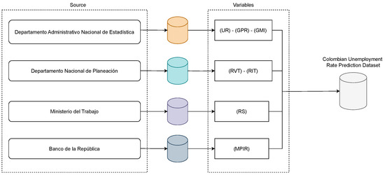
Figure 1.
The Colombian Unemployment Rate Prediction Dataset, which includes Real Salary (RS), Real Income Tax (RIT), Real Value-Added Tax (RVT), Monetary Policy Intervention Rate (MPIR), General Participation Rate (GPR), Economic Monitor Index (EMI), and Unemployment Rate (UR).
The primary values of RS, RIT, and RVT are deflated based on the 2018 level, as recommended by DANE. No missing values were found in the dataset. A detailed summary of the variable notation and their respective data sources is provided in Table 1.

Table 1.
Colombian Unemployment Rate Prediction Dataset notation and sources.
An exploratory description of the dataset has been incorporated to enhance the analysis. The dataset descriptive statistics are presented in Table 2, which enables the characterization of their magnitude, dispersion, and central tendency over the 2005–2023 period. Heterogeneous economic dynamics and the potential presence of structural effects are suggested by the high variance of variables such as RS, RIT, and RVT. In contrast, UR maintains an average of 11.0% and a moderate standard deviation, which indicates that the economy is susceptible to economic disruptions and that unemployment is persistent.
Table 2.
Colombian Unemployment Rate Prediction Dataset descriptive statistics.
Finally, the scatterplot matrix among the studied variables is illustrated in Figure 2, which facilitates the identification of bivariate relationships and marginal distributions. Variables such as GPR and EMI are known to concentrate within specific ranges along the diagonals, while others, such as RIT and RVT, exhibit asymmetries or the prevalence of long tails. Additionally, the bivariate analysis demonstrates positive correlations between RS and EMI, as well as between RIT and RVT, which are in accordance with the interaction between fiscal revenue and economic activity. In contrast, variables such as RS or EMI are associated with an inverse relationship with UR.
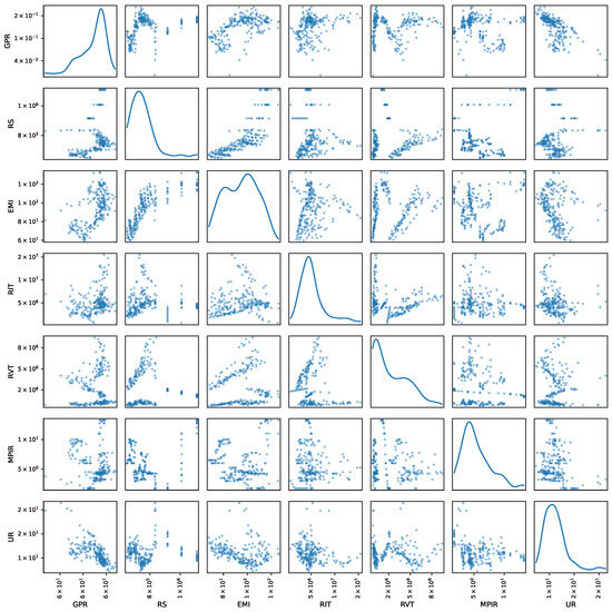
Figure 2.
Pairwise relationships between the socioeconomic and monetary variables (Colombian Unemployment Rate Prediction Dataset). Diagonal elements show univariate distributions, while off-diagonal elements display bivariate scatter plots.
2.2. Nonlinear Unsupervised Relevance Analysis Using UMAP-Based Local Biplots
Given an input feature matrix, (with , P-dimensional features and N samples), a lower-dimensional UMAP-based embedding, , with , is performed in the following two steps: (i) Constructing a weighted k-nearest neighbor (k-NN) graph from a given pairwise Euclidean distance matrix, , to measure the relationships between instances . (ii) Estimating a low-dimensional embedding that preserves the input data structure. Namely, the k-NN graph is initially built from , holding edges defined by a local connectivity through the following weight matrix with elements:
where serves as a normalization factor to define a local measure at point , and rules outlier distances within the n-th neighborhood. To ensure a symmetric diffuse measure, the weights in Equation (1) are normalized as:
In turn, a low-dimensional weight matrix is computed as:
where denote points in the low-dimensional embedding space, and are hyperparameters—typically set to 1—that control the trade-off between preserving local and global structures. The UMAP optimization objective can then be formulated as a cross-entropy loss function:
UMAP allows clustering in the lower-dimensional latent variable space, where clusters may be more apparent, particularly through the K-means clustering algorithm [43]:
where is the number of disjoint sets with , and is d-th partition center.
For enabling a better understanding of UMAP clustering, the SVD biplots are employed in this study to combine the partition set with a reduced representation of the high-dimensional original feature matrix, linearly projecting a d-th cluster as:
where is the low-dimensional representation computed by the 2D singular value decomposition, as follows:
where notation stands for the Frobenius norm. So, the projection term is computed as where is the diagonal matrix holding the singular value decomposition. Nonetheless, we ensure that the non-linear UMAP technique preserves the feature structure during the reduction process using an affine-like transformation [56]:
where and the terms encode a composition of rotation, dilation, shears, and translation-based linear functions. Lastly, a localized feature ranking vector can be computed as:
2.3. Autoregressive Models and Machine Learning Regression
A range of autoregressive and machine learning approaches are employed to investigate the relationships between dependent variables and their corresponding independent indicators. The most commonly used models include:
- Autoregressive Integrated Moving Average (ARIMA): An ARIMA model is utilized to detect stationary correlations within time series data. The mathematical representation is articulated by the subsequent equation, wherein, for simplicity, it is presumed that both the autoregressive and moving average components possess identical lags:In this formulation, represents the time series at time t, whereas signifies a constant. The collection of observations encompassing the pertinent delays is denoted by . Furthermore, the series’ lags are represented by , while the associated coefficients of the autoregressive component are organized in , where signifies the quantity of lags under consideration.Conversely, denotes a white noise process and gathers the moving average coefficients.The ARIMA model can be expressed in matrix notation as follows:where and . The model coefficients are represented as , where .When the aforementioned approach is adapted to encompass seasonal patterns, the ARIMA model is converted into a Seasonal Autoregressive Integrated Moving Average (SARIMA). This comprehensive approach encompasses both stationary correlations and seasonal changes within the data. The general form, assuming that the seasonal components display the same lag as the non-seasonal components, yields:Next, the matrix-based representation is as follows:where and signify the seasonal autoregressive component, with indicating the number of lags. Likewise, and represent the seasonal moving average white noise process and its corresponding coefficients. In both instances, denotes the quantity of periods employed to illustrate seasonality.Also, the SARIMA model can be represented in its concise version as: , with , where . Simultaneously, the parameter vector yields: , where .Notably, ARIMA and SARIMA models are typically optimized using Maximum Likelihood Estimation (MLE), where the parameter estimation process is often carried out via the Limited-memory Broyden–Fletcher–Goldfarb–Shanno with Box constraints (L-BFGS-B) algorithm—a quasi-Newton method well-suited for high-dimensional problems with bound constraints [57].
- Ordinary Least Squares (OLS): This methodology presupposes a linear correlation between the exogenous variables , consisting of N samples and P features, and a target variable . Then, a linear relationship is fixed as , where the coefficient vector represents the parameters that characterize the linear influence of each feature on the target variable. A commonly employed method for estimating the OLS coefficients involves the Moore–Penrose pseudoinverse, leading to the closed-form solution:A regularized extension of the OLS method can be derived by solving the following optimization problem:Notably, when and , OLS yields to L1 regularization, or Least Absolute Shrinkage and Selection Operator (LASSO). Likewise, when the combination of L1 and L2 regularization—commonly referred to as Elastic Net regression—emerges as the resulting formulation [43].
- Random Forests (RF): Let be the target vector and denote the exogenous input feature matrix. An RF-based non-linear prediction is defined as:where the j-th tree codes whether the observation is associated with a node l and tree j. Conversely, the parameters linked to each node are denoted as , representing the coefficients connected with each node in the respective trees. Then: holds the set , delineating the input space partitions created by each tree. The matrix consolidates the indicator functions of all trees and represents the aggregation of the coefficients.RF determines the optimal split criteria and decision thresholds by leveraging the Classification and Regression Trees (CART) algorithm, which iteratively partitions the data to minimize the following classification or regression error [58]:
- Support Vector Regression (SVR): Given an input sample , the non-linear SVR’s predictive function is formulated as follows:where is a coefficients vector and denotes the function that transforms the data into a higher-dimensional space, with . This transformation presents a computational burden, which is mitigated by the kernel trick, allowing the computation of the inner product in the transformed space without direct evaluation [59]. Thus, for two samples, the kernel function is delineated as:The resultant matrix is represented as . Subsequently, a dual optimization formulation is employed to derive the SVR prediction function, enabling efficient computation in high-dimensional feature spaces:In this context, and represent the support coefficients. SVR employs the Sequential Minimal Optimization (SMO) approach to tackle a quadratic programming optimization, articulated as follows [60]:where
Consequently, the formulation of the minimization problem associated with each regression varies depending on the selected modeling strategy, e.g., linear vs. non-linear, and the type of regularization applied. These elements significantly influence both the computational complexity of the solution and the model’s capacity to generalize when exposed to unseen data. Moreover, the relevance of each input feature is typically reflected in the model parameters, whose interpretation depends on the specific supervised framework employed. In the case of ARIMA and SARIMA linear models, feature relevance is inferred from the seasonal and non-seasonal autoregressive coefficients, which encapsulate the influence of past observations on the temporal dynamics of the series.
In contrast, OLS regression provides an explicit quantification of the influence that each exogenous variable exerts on the dependent variable through the estimated coefficients. This approach stands in opposition to autoregressive models, which primarily capture the intrinsic temporal dependencies within the series itself. In the case of RF, interpretability is achieved through the analysis of variable importance, typically measured by either the reduction in node impurity or the change in predictive accuracy resulting from the inclusion or exclusion of each feature [61]. Conversely, SVR does not inherently offer a straightforward mechanism for evaluating variable importance due to its reliance on margin-based optimization and kernel functions [62]. As a result, auxiliary interpretability techniques—such as Shapley value decomposition or sensitivity analysis—are often required to estimate the individual contribution of each feature [63].
2.4. Supervised Kernel-Based Relevance Analysis Using Gaussian Processes
Considering an input involving exogenous variables and a target variable , a Gaussian Process (GP) regression fixes a prior on the coefficient vector , where represents a covariance matrix. The mean and variance of the prediction function are calculated as:
and:
As a result:
where notation stands for a Gaussian-based probability function.
In GP-based regression, the observed outputs are modeled as noisy realizations of an underlying latent function. Assuming additive Gaussian noise, the model is expressed as: , where represents independent and identically distributed Gaussian noise. Consequently, the marginal likelihood of the observed outputs , conditioned on the input matrix , follows a multivariate normal distribution:
where is the covariance matrix defined by the GP kernel, and accounts for the observation noise covariance.
Given a new input , GP regression computes the predictive probability distribution by conditioning the joint Gaussian prior on the observed data. This results in a closed-form expression: , with predictive mean and variance as follows:
where
Of note, the GP regression typically finds the kernel hyperparameters by maximizing the marginal likelihood (also called the evidence) of the observed data. This process balances model fit and complexity in a principled, probabilistic way. Thereby, the L-BFGS-B algorithm is used to solve the following optimization problem:
where notation highlights the kernel dependency on the hyperparameter set
To enable non-linear and supervised regression within a probabilistic framework that leverages kernel-based mappings and prior-informed weight regularization, we enhance input feature relevance analysis to improve a GP-based model’s interpretability. Specifically, we employ a squared exponential kernel—a.k.a. radial basis function (RBF)—with distinct lengthscales assigned to each input dimension:
where and . Then, each lengthscale can be optimized as in Equation (26) to quantify the p-th feature relevance regarding the GP’ predictions. In this context, the p-th feature supervised relevance value is defined as the reciprocal of , yielding:
where a reduced value of indicates the model’s enhanced capacity to detect local fluctuations in the associated feature. Conversely, a bigger value indicates a more diffuse effect, signifying diminished influence on the forecast.
Figure 3 depicts the key principles discussed in this section. This graphic representation highlights both unsupervised (UMAP-based local biplots) and supervised (GP-based regression) approaches for explainable unemployment rate prediction. Notably, the UMAP-Base Local Biplot (UL-Biplot) method is utilized during the unsupervised phase, whereas GP-based regression with kernel relevance analysis is employed in the supervised stage. This strategy facilitates a comparative assessment of interpretability across both paradigms: UL-Biplot uncovers latent patterns and underlying structures without supervised constraints, while GP offers an interpretation grounded in the target variable, the unemployment rate.
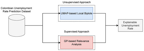
Figure 3.
Explainable framework for unemployment rate prediction in Colombia. (Top): UMAP-based Local Biplot (unsupervised). (Bottom): GP-based relevance analysis (supervised).
3. Experimental Set-Up
3.1. Assessment and Method Comparison
To test our dual framework for explainable unemployment rate prediction, we compute the Pearson’s correlation coefficient to quantify feature relevance from UL-Biplot, defined for two features, p and , as follows:
where denotes the p-th column of the data matrix , while refers to the -th row of the matrix , see Equation (6), which comprises features derived from the UL-Biplot. The vector is utilized to center the data by subtracting the mean .
Now, in the supervised phase, a GP is utilized to forecast the unemployment rate, emphasizing the importance of the hyperparameter set as a tool for interpretability. These lengthscale-related hyperparameters enable the assessment of each feature’s relative contribution to the variability of the economic phenomenon. Then, to assess the efficacy of the supervised models, conventional measures are utilized, contrasting the reference with the prediction , defined as follows:
SVD-based Biplot (SVD-Biplot) is incorporated as a method comparison for unsupervised explainablity [64]. This approach facilitates the visualization and examination of feature significance within the latent framework of the data.
Furthermore, to assess the efficacy of our GP-based unemployment prediction and supervised relevance analysis, its outcomes are compared with the following techniques:
- Autoregresive approaches: ARIMA and SARIMA decompose the series into trend, seasonality, and noise components to encapsulate temporal dynamics [65,66].
- Linear Machine Learning: Lasso and ElasticNet utilize regularization to improve generalization and facilitate variable selection in high-dimensional contexts [67,68].
- Nonlinear Machine Learning: RF and SVR, which adeptly capture intricate interactions and non-linearities in the data using ensemble learning and kernel-based methodologies, respectively [69,70]. Also, a Multilayer Perceptron (MLP) is regarded as a supplementary non-linear benchmark due to its proven ability to predict complex temporal and economic patterns via deep and adaptable feature representations [71].
3.2. Training Details
Regarding the UL-Biplot, the dimensionality is reduced to two, with a minimum distance of 0.75 and the number of neighbors defined as , where stands for the round operator. Furthermore, a silhouette score-based analysis is carried out to fix the number of clusters to improve the visualization of data distribution and evaluate the impact of each variable on the UMAP-based latent representation, as follows:
where is the average distance between point n and all other points in the same cluster (intra-cluster distance) and is the minimum average distance from point n to all points in the nearest neighboring cluster (nearest-cluster distance).
In turn, to evaluate the unemployment rate prediction performance in a time-dependent setting, two cross-validation strategies are applied: Time Series Cross-Validation (TSCV) and Sliding Window Cross-Validation (SWCV) [72,73]. In the former, the training set incrementally enlarges in each iteration by integrating new observations. Conversely, the latter employs a fixed-size window, wherein the oldest data points are eliminated as new observations are incorporated. Both methodologies considered time-frames of 3 and 12 months for the unemployment rate analysis [74]. For both study schmes, corresponding to prediction steps of 3 and 6 months, distinct modeling methodologies are utilized based on the task’s nature. In the unsupervised context, SVD-Biplot and UL-Biplot depend exclusively on the initial values of the seven principal variables (GPR, RS, EMI, RIT, RVT, MPIR, UR) in conjunction with temporal identifiers (Year and Month), omitting lagged features. Conversely, ARIMA and SARIMA models are optimized through the auto_arima function employing a stepwise search, with the maximum lag order established at 3 and seasonal periodicity selected as either 12 or 3, contingent upon the temporal resolution (see to Equations (8) and (10)). These models are trained solely with the UR variable, utilizing internal optimization to capture temporal dependencies without supplementary exogenous inputs. In supervised models—RF, SVR, GP, MLP, Lasso, and ElasticNet—the feature space is established by implementing a fixed 5-month lag window on each of the seven variables, which offers a temporally enhanced representation that facilitates the learning of short-term dynamics. This procedure increases the feature set from 7 to 41 variables. The complete setup is encapsulated in Figure 4. Hyperparameters are refined by grid or randomized search methods. The Lasso penalty coefficient is chosen from the interval , whereas ElasticNet adjusts both the L2 penalty and L1 ratio within the range . Random Forest optimizes max_depth and n_estimators within the range of ; Support Vector Regression assesses linear, polynomial, RBF, and sigmoid kernels, adjusting and ; Gaussian Processes utilize RBF kernels with lengthscales spanning and regularization parameters ranging from ; Multi-Layer Perceptron configurations consist of one or two hidden layers containing units (step 2), various activation functions (relu, tanh, sigmoid, selu, linear), and a solitary relu-activated output neuron. Optimization is performed via adam, rmsprop, sgd. The relevance analysis based on Gaussian Processes is further enhanced using KerasTuner (v1.4.7) [75,76].
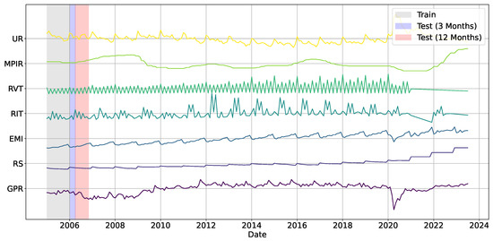
Figure 4.
Illustrative sketch of unemployment rate prediction using fixed lag structures applied to the selected input variables. Shaded regions indicate the training lag and the two forecasting horizons: light blue for the 3-month test and light red for the 12-month test.
All experiments are conducted in Python 3.10.12 within the Google Colaboratory environment, employing several libraries including scikit-learn (version 1.6.1), umap-learn (version 0.5.7), statsmodels (version 0.14.4), and pmdarima (version 2.0.4). A detailed depiction of the experimental configuration is illustrated in Figure 5 and our codes with the studied datasets are publicly available at https://github.com/UN-GCPDS/Unemployment-Rate-Prediction.git, (accessed on 1 April 2025).
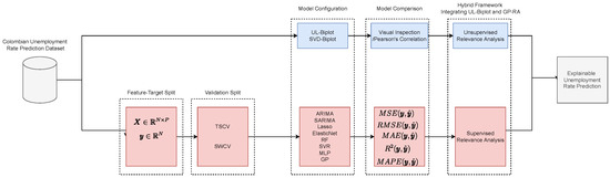
Figure 5.
Explainable unemployment rate prediction pipeline. (Top): UMAP-based local biplots (unsupervised). (Bottom): GP-based relevance analysis (supervised). UL: UMAP Local Biplot.
4. Results and Discussion
4.1. Unsupervised Relevance Analysis
Figure 6 presents the silhouette coefficients [43] (indicated by the vertical red line) computed for different clustering configurations within our UL-based approach, varying the number of clusters from three to six. These plots serve as a diagnostic tool to evaluate clustering quality and guide the selection of an optimal partitioning scheme. Although the silhouette profiles are relatively comparable across all configurations—none displaying coefficients below the average threshold—cluster solutions with four and five groups yield more balanced distributions in terms of the number of points per cluster. In contrast, configurations with three and six clusters exhibit greater heterogeneity in cluster shapes and sizes. Notably, the silhouette coefficient attains its maximum value at five clusters but does not improve consistently with additional groupings. Consequently, a five-cluster solution is recommended as it offers a compromise between cluster compactness, separation, and balance, ensuring a robust latent structure interpretation.
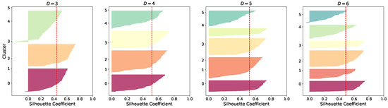
Figure 6.
UL-based silhouette coefficient obtained for clustering results. Vertical dashed lines represent the silhouette scores for each group.
Next, Figure 7 presents the unsupervised relevance analysis results of the visual inspection performed on the Colombian unemployment rate dataset. In each projection, the basis vectors (represented as arrows) illustrate the contributions of the original variables. Arrows are color-coded according to their associated socioeconomic and monetary variable categories, enhancing interpretability. Additionally, 2D embeddings are displayed with UR values mapped to a color gradient, offering further insight into spatial distribution and density. The results reveal notable variability and structural complexity within the dataset.
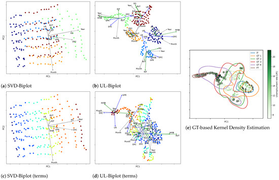
Figure 7.
Different visual inspection results based on SVD-Biplot and UL-Biplot: (a,c) depict the SVD-Biplot colored by clustering label and Government terms, respectively. (b,d) showcase UL-Biplot method with colors representing the clustering label and Government terms, respectively. (e) Local Biplot and cluster-based probability boundaries. The plot’s color emphasizes the target variable (UR), while the Goverment Terms (GT) Initial (IT), GT 1-4, Final (FT), determine the color of the curves. Markers indicate specific events: diamonds represent the crisis period of 2008, while squares denote the COVID-19 pandemic period (2019–2023). PC: principal component (basis).
The SVD-Biplot displays a wide dispersion of samples with substantial cluster overlap, indicating poor separation and reduced interpretability compared to the UL-Biplot, which reveals more defined group structures. Among the variables, Year and RS exhibit the longest vectors, both aligned with PC1, suggesting they are the dominant drivers of variance in the first principal component. In contrast, Month, UR, and RVT align with PC2, with Month contributing the most prominently in that direction. The close alignment between Year and RS also points to a strong positive correlation between these variables. Meanwhile, the relatively shorter arrows for UR and RVT indicate limited influence on the second principal component. Altogether, the structure unveiled by these projections suggests a nontrivial data arrangement, with significant internal variability likely reflecting latent subgroups or non-stationary temporal dynamics embedded within the dataset.
In contrast, the UL-Biplot excels in preserving local structures, resulting in the formation of tighter, well-defined clusters that effectively highlight latent subgroups within the data. The corresponding 2D non-linear embedding, scaled to the range , captures not only the broad global geometry of the dataset but also retains critical local relationships, yielding a configuration of compact and coherent clusters. The color-coded arrows offer further insight into variable contributions, indicating that socioeconomic variables (shaded in blue) play a more prominent role than monetary indicators in shaping the observed variability across clusters. Noteworthy correlations emerge, particularly between RS and RVT, while EMI consistently exhibits strong positive and negative correlations with GPR and UR, respectively, across all identified groups. Overall, our UL-based clustering consolidates economic variables that affect the unemployment rate. Assessment of their importance demonstrates that unemployment dynamics are closely associated with wage trends and overall economic activity. This finding aligns with macroeconomic theory, which highlights the interrelationship between the labor market, business cycles, and monetary policy. In this context, both seasonality (months and periods of the year) and long-term trends (years) substantially impact fluctuations in unemployment.
Additionally, the embedding space reveals a temporal dimension, with distinct structural contours aligning with different presidential administrations. This temporal stratification underscores the dynamic nature of inter-variable relationships and provides crucial context for interpreting seasonal patterns, policy shifts, and other time-dependent socio-economic dynamics affecting the Colombian labor market. Indeed, when generating the UL for each cluster based on the government terms variable, the resulting projections showed significant overlap between clusters. This suggests that the chosen variable, does not provide sufficient separation to distinguish the groups effectively. The difficulty in interpreting these biplots is a direct consequence of the poor differentiation, as the projections from different sets occupy similar regions of the biplot space, indicating that government terms may not be the most suitable criterion for partitioning the data. Additionally, the dispersion of samples could be attributed to noise or variability in the data or shared contextual factors across different government terms. This highlights the complexity of the dataset, where temporal or policy similarities may lead to overlapping clusters.
The local biplot framework enables a thorough examination of each cluster feature relevance analysis, as illustrated in Figure 8 and Figure 9. For cluster 1, MPIR exerts a significant influence on UR. Monetary policy theoretically affects credit availability and investment conditions, thereby influencing the business cycle and, consequently, employment levels. The Pearson correlation-based assessment identifies GPR, EMI, and RVT as primary determinants; see Figure 9. The proposed approach posits that MPIR plays a crucial role, supporting the hypothesis that variations in intervention rates can affect labor supply and, subsequently, unemployment. Moreover, cluster 2 shows that fiscal impact is demonstrated through RVT, which reflects the interplay of tax revenue and its influence on the tax base and employment incentives. Also, RIT, RS, and EMI exhibit high relevance. The Pearson correlation emphasizes GPR, EMI, and MPIR, while the inclusion of RIT in the analysis demonstrates that fiscal policy, through changes in direct taxation, can significantly affect the labor market, particularly in terms of business profitability and job creation.
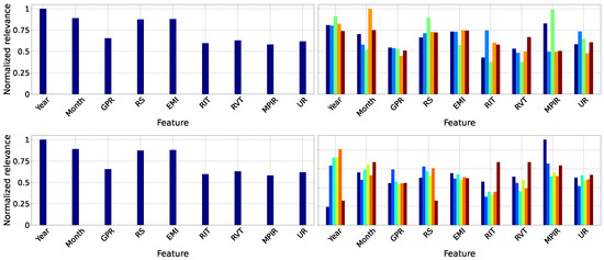
Figure 8.
Unsupervised feature relevance analysis. Left: SVD-Biplot. Right: UL (ours). First row: Input data feature relevance. Second row: Government terms-based results. The bar color in the second column stands for UL clusters labels (see Figure 7b,c).
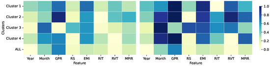
Figure 9.
Pearson correlation results. Left: SVD-Biplot, Right: UL (ours). We show the absolute correlation between the features and the unemployment rate (target) for each cluster separately and throughout the dataset.
Cluster 3 exhibits a pronounced sensitivity of the unemployment rate to variations in MPIR and RS, as depicted in Figure 8. While the Pearson correlation analysis focuses solely on EMI as an explanatory variable, the local biplot reveals a broader interaction that also encompasses RS and RIT, as depicted in Figure 9. This result aligns with aggregate demand theory, which posits the influence of wages and public expenditure on employment levels. Cluster 4 concurrently emphasizes the interaction between fiscal variables (RIT and RVT) and economic factors (EMI and RS). The Pearson correlation for SVD-Biplot indicates a strong relationship with RS and EMI, while the proposed method broadens the scope of relevant factors by including GPR, MPIR, and RIT. This highlights the diverse mechanisms through which fiscal policies (direct and indirect taxation) and monetary measures (MPIR) affect labor supply and demand. Likewise, cluster 5 identifies EMI, RS, and RVT as significant variables, further demonstrating the influence of fiscal policy and economic activity on the labor market. In alignment with Cluster 4, Pearson correlation via SVD-Biplot supports these findings, while the local biplot provides a more nuanced view of the determinants affecting the unemployment rate. Remarkably, clusters 4 and 5 share similar patterns in variable importance and inter-variable correlations, with key distinctions emerging in the influence of fiscal (RVT, RIT) and monetary (MPIR) factors. A detailed analysis of these variables reveals their temporal relevance and explanatory power in understanding Colombian unemployment trends. So, the proposed UL-based framework effectively uncovers meaningful relationships among economic indicators, offering a refined lens for economic interpretation.
Lastly, the KDE analysis (Figure 7e) highlights that major economic events—such as the COVID-19 pandemic during Iván Duque’s presidency (GT4), the early term of Gustavo Petro (FT), and the 2008 global financial crisis under Álvaro Uribe—are distinctly mapped into separate clusters. These periods align with specific economic signatures: for instance, RS, MPIR, Year, and Month characterize the green cluster, while Month, MPIR, and EMI define the dark blue cluster in the Local Biplot (Figure 7b). Consequently, our proposal allows capturing structural economic shifts and supporting the evidence-based design of public policies, grounded in theoretical and data-driven insights.
4.2. Supervised Relevance Analysis
Figure 10 presents the time series of the Colombian unemployment rate alongside the forecasts generated by various predictive models (ARIMA, Lasso, Elastic-Net, and GP), as well as their decomposition into trend, seasonality, and residual components, performed using Equation (8). The results highlight that the effectiveness of a validation strategy is inherently tied to the selected temporal analysis window, underscoring the importance of preserving the chronological structure during model evaluation. The plots reveal significant structural changes aligned with major economic events. Notable examples include the spike in unemployment during the 2007–2008 global financial crisis (first shaded region), the sustained economic decline across Juan Manuel Santos’s administration (2010–2018), and the sharp rise during the COVID-19 pandemic (second shaded region). These findings demonstrate the models’ ability to detect abrupt regime shifts and temporal discontinuities while reinforcing the critical need for validation techniques that respect the sequential nature of time series data, ensuring robust and context-aware forecasting performance. Moreover, the decomposition analysis reveals that the seasonal component exhibits a stable and recurring annual pattern, particularly pronounced toward the end of each year, when unemployment rates typically decline. This trend is attributed to increased labor demand during the holiday season, driven by temporary employment opportunities, which contribute to a short-term reduction in unemployment levels. Recognizing such seasonal regularities highlights the importance of integrating cyclical features into forecasting models, allowing algorithms to more accurately capture and adapt to recurrent fluctuations within the time series.
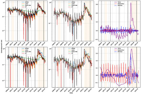
Figure 10.
Unemployment rate prediction results. Comparison of the estimates from the best models against the original signal (in black): ARIMA, Lasso, Elastic-Net, and GP are tested. At the Top, a 3-month prediction window is shown, while at the Bottom, a 12-month window is used. Left: results obtained through TSCV. Middle: results with SWCV. Right: seasonal decomposition of the unemployment rate (trend in purple, seasonality in red, residuals in blue).
The progression of inferences within each validation window enables a comparison between econometric models, such as ARIMA, and machine learning methods, including Lasso, Elastic-Net, and GP. The findings demonstrate that ARIMA inadequately represents the series’ dynamics, while Lasso yields results similar to traditional methods. Conversely, GP attains high accuracy in short-term predictions within the time series cross-validation framework; however, its efficacy declines under sliding window validation and in 12-month forecasting horizons, revealing considerable sensitivity to data availability. This contrast underscores the significance of choosing both the suitable model and the most efficient validation method to guarantee consistent outcomes. Throughout the COVID-19 pandemic, all models demonstrated a reduction in accuracy, indicating the influence of abrupt changes in unemployment trends and the restricted data availability in this unparalleled situation. Figure 10 (second column, second shaded area) demonstrates how the escalation in both the trend and residual components exposed the difficulties encountered by these methodologies. Nonetheless, the continuity of the annual seasonal cycle indicates that these patterns persistently affect unemployment trends, even during disruptive occurrences.
Figure 11 illustrates the progression of two hyperparameters over three- and twelve-month intervals to evaluate model stability. The findings demonstrate significant discrepancies in ARIMA and ElasticNet hyperparameters during model inference, suggesting a propensity for overfitting that limits generalization. Conversely, GP demonstrates superior stability in its hyperparameters, indicating improved generalization capability and resilience. This attribute renders it a dependable choice in situations where adaptability and precision are crucial, especially in time series exhibiting considerable temporal variability. Despite initial fluctuations, hyperparameters generally stabilize during the pandemic, corresponding with the progression of the series’ patterns. This behavior can be attributed to economic contraction, heightened public expenditure, diminished tax burdens, and reduced monetary policy intervention. These factors established a deflationary environment that, according to economic theory, is associated with a moderate reduction in employment. The decrease in the volatility of essential indicators, including interest rates and production levels, streamlined the data structure, facilitating the recognition of more stable patterns. As a result, consumption-fueled economic recovery enabled employment levels to revert to pre-pandemic conditions [77]. The stabilization of the economic cycle aided in preserving consistency in the models’ learning processes, notwithstanding fluctuations in macroeconomic conditions.
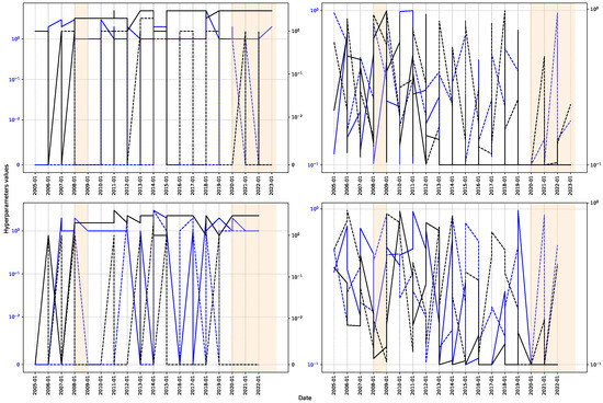
Figure 11.
Hyperparameter analysis. The solid line represents the behavior with TSCV, while the dashed line shows the behavior with SWCV. At the top, a 3-month window is analyzed, while at the bottom, a 12-month window is used. Left: hyperparameters corresponding to the autoregressive lag order (in blue) and the moving average lag order (in black) of the ARIMA model are presented. Right: l1_ratio (in blue) and alpha (in black) for Elastic-Net are illustrated.
Table 3 provides a comparative analysis of different regression models utilizing various metrics and validation techniques applied in this study, focusing on two analysis windows. A three-month forecasting horizon is employed to evaluate model efficacy in the initial case. In TSCV, training and test sets are developed cumulatively, progressing through the series without including future data in the training, thus maintaining the sequential integrity of the problem. Conversely, SWCV utilizes a fixed-length window that advances prior to each prediction, enabling the elimination of outdated observations and accommodating possible alterations in the temporal distribution. This distinction is essential, as each method offers particular advantages based on the historical development of the series or the necessity for adaptability to structural changes.
Table 3.
Unemployment rate prediction method comparison results (3-month prediction window). TSCV: Time Series Cross-Validation; SWCV: Sliding Window Cross-Validation.
The findings indicate that traditional models, including ARIMA and SARIMA, display greater errors and markedly reduced values in comparison to machine learning approaches. In contrast, methodologies such as Lasso, ElasticNet, SVR, and GP exhibit enhanced effectiveness owing to their capacity to discern intricate patterns and address data uncertainty. ARIMA and SARIMA often oversimplify temporal dynamics by presuming stationarity or consistent seasonality, while machine learning models provide enhanced flexibility and accuracy, especially in the context of non-linear relationships or structural alterations within the series. This comparison validates the superiority of contemporary methods in encapsulating the intrinsic complexity of economic data.
Then, As the forecasting horizon reaches 12 months, as illustrated in Table 4, the efficacy of all methodologies markedly diminishes. However, the previously observed trend persists: as the time horizon extends, the amount of relevant information for future projections decreases, impairing the model’s predictive performance. Despite this decline in precision, machine learning methods continue to outperform traditional econometric approaches, reaffirming their suitability for modeling time series with complex structures.
Table 4.
Unemployment rate prediction method comparison results (12-month prediction window). TSCV: Time Series Cross-Validation; SWCV: Sliding Window Cross-Validation.
Specifically, in the comprehensive examination of the Lasso model (Figure 12, top panel), the variables with the highest weights are RS, indicative of household purchasing power and, by extension, consumption, and EMI, denoting the vigor of national economic activity. RVT comes third in significance, reflecting the effect of indirect taxation on consumer expenditure, whereas RIT encompasses the impact of direct taxes on disposable income. Conversely, GPR and MPIR demonstrate a relatively less impact, as labor force participation and financing costs exert a less pronounced influence on unemployment dynamics within this linear model.
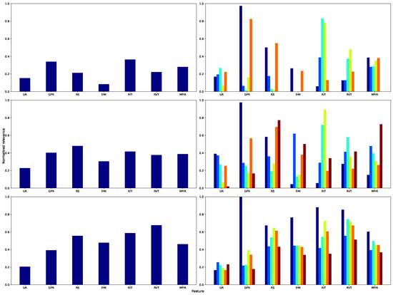
Figure 12.
Supervised feature relevance analysis across different models. Left: Normalized mean relevance for each feature. Right: Normalized feature relevance by Government terms, with bar colors indicating cluster labels (see Figure 7c). Each row corresponds to a different model: Lasso (top), RF (middle), and GP (bottom).
Moreover, when analyzed by governmental administrations, the IT stage underscores the significance of the monetary intervention rate, as fluctuations in credit costs swiftly influence investment and employment levels. Throughout GT1 and GT2, EMI and the progression of UR dominate, acting as markers of the business cycle’s expansionary and contractionary stages. In GT3 and GT4, the significance of RS and RVT highlights the importance of real wages and VAT in influencing labor demand. Ultimately, in FT, the proportional increase in GPR indicates an augmentation in labor supply associated with measures designed to foster inclusion.
In addition, the RF algorithm (Figure 12, center panel) highlights the significant importance of RVT and MPIR, underscoring the influence of non-linear effects arising from fiscal and monetary policy. Alterations in VAT and modifications to the intervention rate are crucial for understanding intricate relationships among consumption, investment, and employment. Nonetheless, RS and EMI maintain their significance by indicating purchasing power and the economic cycle. An analysis of governmental periods indicates that IT and GT1 are significantly influenced by indirect taxation on UR. In GT2 and GT3, this effect is counterbalanced by the influence of EMI and RS, whereas in GT4 and FT, MPIR becomes a crucial factor, underscoring the importance of capital costs in employment dynamics during transitional periods.
Similarly, the GP (Figure 12, bottom panel) demonstrates that shorter lengthscales in MPIR and RVT signify an increased sensitivity of UR to minor variations in the monetary policy rate and consumption-related tax burden. RS and EMI exert a significant effect by monitoring fluctuations in aggregate demand and business cycles. Besides, GPR assumes a subordinate position, as labor supply reacts more slowly to macroeconomic disturbances. IT demonstrates a more pronounced reaction of UR to MPIR modifications; in GT1 and GT2, EMI and RS predominantly account for variability; in GT3 and GT4, RVT emerges as the primary factor; and in FT, the growing influence of RS indicates policy initiatives focused on enhancing labor income in the latest phase of the cycle.
Finally, the comparative analysis reveals that the upper quartiles of relevance for the supervised strategy (GP) and the unsupervised method (UL), illustrated in Figure 13, exhibit a common set of variables: GPR, RIT, and RS. This convergence highlights their essential function in simulating the evolution of unemployment in Colombia. Notably, GPR, as an indicator of labor force participation, reflects the labor market’s sensitivity to macroeconomic variations. Its significance in both methodologies affirms its structural importance in economic adjustment processes. Simultaneously, RIT illustrates the effect of fiscal policy on disposable income and employment incentives, indicating that direct taxation can affect labor market choices on both the supply and demand sides. Furthermore, RS signifies real wage circumstances, which directly influence income expectations and household consumption ability. This connection creates a robust association between the labor market and the aggregate demand.
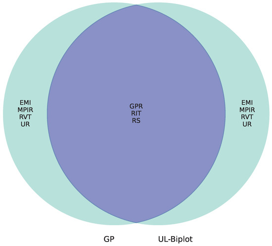
Figure 13.
Unsupervised (UL) and Unsupervised (GP) feature relevance comparison. Left: Supervised relevance analysis (GP). Middle: Overlap showing features identified as relevant by both approaches. Right: Unsupervised relevance analysis (UL-Biplot).
4.3. Limitations
While the proposed framework demonstrates promising results in enhancing interpretability and predictive accuracy for unemployment rate estimation, several limitations must be acknowledged. First, the current approach is predominantly data-driven and does not yet incorporate a structural economic model grounded in established macroeconomic theory, such as the Phillips Curve or the concept of a Natural Rate of Unemployment (NAIRU). These frameworks offer essential insights into long-term labor market equilibria and the trade-off between inflation and unemployment, especially in dynamic policy environments. Integrating structural modeling—such as the expectations-augmented Phillips Curve—would enhance the theoretical consistency of the forecasting framework and permit deeper causal analysis [78]. Second, the relatively small dataset (228 observations) constrains the generalizability and scalability of the current model. Sample limitations can lead to model variance inflation and reduced performance under unseen economic regimes regarding probabilistic modeling and data sufficiency. Third, the harmonization of unemployment-related variables across varying time and spatial resolutions remains a critical challenge. Macroeconomic data often exhibit structural breaks due to shifts in policy or measurement practices. Discrepancies in aggregation levels across variables (e.g., monthly inflation vs. quarterly GDP) and spatial granularity (e.g., national vs. departmental unemployment rates) complicate the direct inclusion of heterogeneous inputs [79]. Addressing these limitations would not only improve the fidelity of the forecasts but also align the modeling approach more closely with the economic mechanisms underlying unemployment.
5. Conclusions
We introduced an explainable hybrid framework for forecasting the unemployment rate in Colombia, combining an unsupervised UMAP-based Local Biplot (UL-Biplot) technique with a supervised Gaussian Process (GP) regression enriched by kernel-based relevance analysis. The unsupervised approach successfully uncovered latent structures within the dataset, revealing meaningful clusters aligned with temporal dynamics, such as presidential terms and major economic events, including the 2008 global financial crisis and the COVID-19 pandemic. It also highlighted the predominant role of socioeconomic variables—particularly labor participation, real wages, and economic activity—in shaping unemployment patterns. In parallel, the supervised GP model achieved superior predictive performance over traditional models (e.g., ARIMA, Lasso, ElasticNet, and SVR) in short-term forecasting under time series cross-validation, while maintaining robust feature relevance interpretation through individualized kernel lengthscales. The model also demonstrated increased generalization and stability compared to other machine learning approaches, especially in handling non-linearities and uncertainty during periods of abrupt economic change. Indeed, presidential terms exhibit a clear correlation with our findings, offering valuable context for interpreting the temporal dynamics and structural shifts in Colombia’s unemployment rate. Of note, the recurrent appearance of RS, RIT, RVT, GPR, EMI, and MPIR across various methodological approaches—from traditional econometric models such as ARIMA and SARIMA to regularized machine learning algorithms like Lasso and Elastic-Net, as well as the hybrid UL-Biplot and GP proposal—highlights their crucial influence on the dynamics of Colombian unemployment.
Beyond methodological advancements, the proposed integration of GP-based regression and UL-based unsupervised relevance analysis offers substantial political value for public decision-making. By generating interpretable predictions of unemployment levels, policymakers are empowered to not only anticipate labor market stressors but also to trace back the contributing socioeconomic and monetary factors in a transparent manner. The predictions provided favor the formulation of risk-aware policies, while the UL framework visually maps economic patterns and latent clusters, enabling the identification of vulnerable groups or periods of systemic fragility. Together, these tools support the design of targeted, evidence-driven interventions that can improve labor participation, stabilize employment conditions, and reduce structural inequality—especially in policy contexts where responsiveness, fairness, and accountability are paramount.
As future work, we propose extending the dataset to include regional indicators, which may uncover localized patterns and support the development of more targeted public policies. Additionally, we suggest exploring probabilistic deep learning models, such as GP Deep Kernel Learning or interpretable attention-based architectures, to preserve model explainability while improving generalization under high temporal variability [80,81]. Additionally, key drivers of the predicted unemployment rate—such as government expenditure, foreign investment, and manufacturing employment—will be incorporated for deeper analysis of unemployment trends. Finally, incorporating qualitative information—such as regulatory changes, sociopolitical events, or labor market perception surveys—could enrich the proposed models and enhance their value as decision-making tools grounded in data and economic theory.
Author Contributions
Conceptualization, D.A.P.-R., D.A.M.-C. and A.M.Á.-M.; data curation, D.A.P.-R., D.A.M.-C. and J.C.T.-M.; methodology, A.M.Á.-M. and G.C.-D.; project administration, A.M.Á.-M.; supervision, A.M.Á.-M. and G.C.-D.; resources, D.A.P.-R., J.C.T.-M. and A.M.Á.-M. All authors have read and agreed to the published version of the manuscript.
Funding
Under grants provived by the project: Sistema de visión artificial para el monitoreo y seguimiento de efectos analgésicos y anestésicos administrados vía neuroaxial epidural en población obstétrica durante labores de parto para el fortalecimiento de servicios de salud materna del Hospital Universitario de Caldas - SES HUC (funded by Universidad Nacional de Colombia, HERMES-57661).
Data Availability Statement
The publicly available dataset analyzed in this study can be found at https://github.com/UN-GCPDS/Unemployment-Rate-Prediction.git (accessed on 1 April 2025).
Conflicts of Interest
The authors declare no conflicts of interest.
References
- Zamanzadeh, A.; Chan, M.K.; Ehsani, M.A.; Ganjali, M. Unemployment duration, Fiscal and monetary policies, and the output gap: How do the quantile relationships look like? Econ. Model. 2020, 91, 613–632. [Google Scholar] [CrossRef]
- Chodorow-Reich, G.; Coglianese, J.; Karabarbounis, L. The macro effects of unemployment benefit extensions: A measurement error approach. Q. J. Econ. 2019, 134, 227–279. [Google Scholar] [CrossRef]
- Ozili, P.; Oladipo, O. Impact of credit expansion and contraction on unemployment. Int. J. Soc. Econ. 2025, 52, 205–219. [Google Scholar] [CrossRef]
- Sakamoto, T. Poverty, inequality, and redistribution: An analysis of the equalizing effects of social investment policy. Int. J. Comp. Sociol. 2024, 65, 310–334. [Google Scholar] [CrossRef]
- Hidalgo Villota, M.E. Business cycles in Colombia: Stylized facts. Tendencias 2024, 25, 26–56. [Google Scholar] [CrossRef]
- Sullivan, M. Comprender y predecir la elección del marco de política monetaria en los países en desarrollo. Model. Econ. 2024, 139, 106783. [Google Scholar] [CrossRef]
- Mamo, D.K.; Ayele, E.A.; Teklu, S.W. Modelling and Analysis of the Impact of Corruption on Economic Growth and Unemployment. In Proceedings of the Operations Research Forum; Springer: Berlin/Heidelberg, Germany, 2024; Volume 5, p. 36. [Google Scholar]
- Patwa, P.; Bhardwaj, M.; Guptha, V.; Kumari, G.; Sharma, S.; Pykl, S.; Das, A.; Ekbal, A.; Akhtar, M.S.; Chakraborty, T. Overview of constraint 2021 shared tasks: Detecting english covid-19 fake news and hindi hostile posts. In Proceedings of the Combating Online Hostile Posts in Regional Languages During Emergency Situation: First International Workshop, CONSTRAINT 2021, Collocated with AAAI 2021, Virtual Event, 8 February 2021; Revised Selected Papers 1. Springer: Berlin/Heidelberg, Germany, 2021; pp. 42–53. [Google Scholar]
- Papić-Blagojević, N.; Stankov, B. Analysis of Trends in Youth Unemployment in the European Union: The Role and Importance of Youth Entrepreneurship. In Entrepreneurship and Development for a Green Resilient Economy; Emerald Publishing Limited: Bingley, UK, 2024; pp. 181–204. [Google Scholar]
- Olschewski, S.; Luckman, A.; Mason, A.; Ludvig, E.A.; Konstantinidis, E. The future of decisions from experience: Connecting real-world decision problems to cognitive processes. Perspect. Psychol. Sci. 2024, 19, 82–102. [Google Scholar] [CrossRef]
- Carrino, L.; Farnia, L.; Giove, S. Measuring Social Inclusion in Europe: A non-additive approach with the expert-preferences of public policy planners. J. R. Stat. Soc. Ser. A Stat. Soc. 2024, 187, 231–259. [Google Scholar] [CrossRef]
- Masoud, N. Artificial intelligence and unemployment dynamics: An econometric analysis in high-income economies. Technol. Sustain. 2025, 4, 30–50. [Google Scholar] [CrossRef]
- Da Re, D.; Marini, G.; Bonannella, C.; Laurini, F.; Manica, M.; Anicic, N.; Albieri, A.; Angelini, P.; Arnoldi, D.; Bertola, F.; et al. Modelling the seasonal dynamics of Aedes albopictus populations using a spatio-temporal stacked machine learning model. Sci. Rep. 2025, 15, 3750. [Google Scholar] [CrossRef]
- Chen, X.S.; Kim, M.G.; Lin, C.H.; Na, H.J. Development of per Capita GDP Forecasting Model Using Deep Learning: Including Consumer Goods Index and Unemployment Rate. Sustainability 2025, 17, 843. [Google Scholar] [CrossRef]
- Departamento Administrativo Nacional de Estadística (DANE). Metodología de Estadísticas Laborales. 2025. Available online: https://bibliotecadoctecnica.dane.gov.co/static/documentos/DIG/DEE/DEE_Metodolog (accessed on 1 April 2025).
- Departamento Administrativo Nacional de Estadística (DANE). Metodología de Encuestas Económicas y de Empleo. 2025. Available online: https://bibliotecadoctecnica.dane.gov.co/static/documentos/DCD/EEVV/EEVV_Metodolog (accessed on 1 April 2025).
- Pigazo-López, F.; del Carmen Ruiz-Puente, M. Analysis of the Dynamic Relationships Between Industrial and Environmental Factors and Unemployment Rate. An Econometric Approach. Dyna. Energía Sostenibilidad 2024, 13, 1–13. [Google Scholar] [CrossRef]
- Chakraborty, T.; Chakraborty, A.K.; Biswas, M.; Banerjee, S.; Bhattacharya, S. Unemployment rate forecasting: A hybrid approach. Comput. Econ. 2021, 57, 183–201. [Google Scholar] [CrossRef]
- Woan-Lin, B.; Hui-Mei, T. Economic Impact on Palm Oil Stock Returns in Malaysia, Singapore, and Indonesia: A Nardl Model Analysis. J. Sustain. Sci. Manag. 2024, 19, 195–202. [Google Scholar]
- Shi, X.; Wang, J.; Zhang, B. A fuzzy time series forecasting model with both accuracy and interpretability is used to forecast wind power. Appl. Energy 2024, 353, 122015. [Google Scholar] [CrossRef]
- Onatunji, O.G.; Adeleke, O.K.; Adejumo, A.V. Non-linearity in the Phillips curve: Evidence from Nigeria. Afr. J. Econ. Manag. Stud. 2024, 15, 132–144. [Google Scholar] [CrossRef]
- Gallegati, M.; Gallegati, S. Why does economics need complexity? Soft Comput. 2025, 1–10. [Google Scholar] [CrossRef]
- Nosike, C.J.; Ojobor, O.S.N. Effects of Government Policies on Recessions: Fiscal and Monetary Policy Impact on Unemployment, Poverty, and Inequality. Interdiscip. J. Afr. Asian Stud. (IJAAS) 2024, 10, 1–12. [Google Scholar]
- Advani, B.; Sachan, A.; Sahu, U.K.; Pradhan, A.K. Forecasting Major Macroeconomic Variables of the Indian Economy. In Modeling Economic Growth in Contemporary India; Emerald Publishing Limited: Bingley, UK, 2024; pp. 1–24. [Google Scholar]
- Mero, K.; Salgado, N.; Meza, J.; Pacheco-Delgado, J.; Ventura, S. Unemployment Rate Prediction Using a Hybrid Model of Recurrent Neural Networks and Genetic Algorithms. Appl. Sci. 2024, 14, 3174. [Google Scholar] [CrossRef]
- Mohamed, A.A.; Abdi, A.H. Exploring the dynamics of inflation, unemployment, and economic growth in Somalia: A VECM analysis. Cogent Econ. Financ. 2024, 12, 2385644. [Google Scholar] [CrossRef]
- Saâdaoui, F.; Rabbouch, H. Financial forecasting improvement with LSTM-ARFIMA hybrid models and non-Gaussian distributions. Technol. Forecast. Soc. Change 2024, 206, 123539. [Google Scholar] [CrossRef]
- Boundi-Chraki, F.; Perrotini-Hernández, I. Revisiting the Classical Theory of Investment: An Empirical Assessment from the European Union. J. Quant. Econ. 2024, 22, 63–89. [Google Scholar] [CrossRef]
- Mutascu, M.; Hegerty, S.W. Predicting the contribution of artificial intelligence to unemployment rates: An artificial neural network approach. J. Econ. Financ. 2023, 47, 400–416. [Google Scholar] [CrossRef]
- Capello, R.; Caragliu, A.; Dellisanti, R. Integrating digital and global transformations in forecasting regional growth: The MASST5 model. Spat. Econ. Anal. 2024, 19, 133–160. [Google Scholar] [CrossRef]
- Shavvalpour, S.; Mohseni, R.; Kordtabar Firouzjaei, H. Analysis of the Asymmetric impact of Oil prices, Exchange rates, and their Uncertainty on Unemployment in Oil-Exporting countries. Macroecon. Res. Lett. 2024, 19. [Google Scholar]
- Sow, A.; Traore, I.; Diallo, T.; Traore, M.; Ba, A. Comparison of Gaussian process regression, partial least squares, random forest and support vector machines for a near infrared calibration of paracetamol samples. Results Chem. 2022, 4, 100508. [Google Scholar] [CrossRef]
- Shamsi, M.; Beheshti, S. Separability and scatteredness (S&S) ratio-based efficient SVM regularization parameter, kernel, and kernel parameter selection. Pattern Anal. Appl. 2025, 28, 33. [Google Scholar]
- Xu, B.; Huang, J.Z.; Williams, G.; Wang, Q.; Ye, Y. Classifying very high-dimensional data with random forests built from small subspaces. Int. J. Data Warehous. Min. (IJDWM) 2012, 8, 44–63. [Google Scholar] [CrossRef]
- Wang, Q.; Nguyen, T.T.; Huang, J.Z.; Nguyen, T.T. An efficient random forests algorithm for high dimensional data classification. Adv. Data Anal. Classif. 2018, 12, 953–972. [Google Scholar] [CrossRef]
- Liu, H.; Ong, Y.S.; Shen, X.; Cai, J. When Gaussian Process Meets Big Data: A Review of Scalable GPs. IEEE Trans. Neural Networks Learn. Syst. 2020, 31, 4405–4423. [Google Scholar] [CrossRef]
- Açıkkar, M.; Tokgöz, S. Improving multi-class classification: Scaled extensions of harmonic mean-based adaptive k-nearest neighbors. Appl. Intell. 2025, 55, 1–25. [Google Scholar] [CrossRef]
- Shaker, M.T.; El-Batanouny, H.; Abdelsalam, M.; Helmy, Y. Systematic Review of Machine Learning Approaches in Forecasting Economic Growth and Enhancing Decent Work Opportunities: A Comprehensive Analysis. In Proceedings of the 2024 6th International Conference on Computing and Informatics (ICCI), Cairo, Egypt, 6–7 March 2024; pp. 377–392. [Google Scholar]
- Aoujil, Z.; Hanine, M. A Review on Artificial Intelligence and Behavioral Macroeconomics. In Proceedings of the International Conference on Smart City Applications, Kuala Lumpur, Malaysia, 17–19 May 2024; Springer: Berlin/Heidelberg, Germany, 2024; pp. 332–341. [Google Scholar]
- Alaminos, D.; Salas, M.B.; Partal-Ureña, A. Hybrid ARMA-GARCH-Neural Networks for intraday strategy exploration in high-frequency trading. Pattern Recognit. 2024, 148, 110139. [Google Scholar] [CrossRef]
- Soltani, A.; Lee, C.L. The non-linear dynamics of South Australian regional housing markets: A machine learning approach. Appl. Geogr. 2024, 166, 103248. [Google Scholar] [CrossRef]
- Jung, J.; Wang, Y.; Sanchez Barrioluengo, M. A scoping review on graduate employability in an era of ‘Technological Unemployment’. High. Educ. Res. Dev. 2024, 43, 542–562. [Google Scholar] [CrossRef]
- Murphy, K.P. Probabilistic Machine Learning: An Introduction; MIT Press: Cambridge, MA, USA, 2022. [Google Scholar]
- Simionescu, M. Machine Learning vs. Econometric Models to Forecast Inflation Rate in Romania? The Role of Sentiment Analysis. Mathematics 2025, 13, 168. [Google Scholar] [CrossRef]
- Mutie, C.K.; Macharia, J.N. Gendered Analysis of the Effect of Displacement on Labor Market Outcomes: A Focus on Nairobi County, Kenya. Economies 2025, 13, 51. [Google Scholar] [CrossRef]
- Orozco-Castañeda, J.M.; Sierra-Suárez, L.P.; Vidal, P. Labor market forecasting in unprecedented times: A machine learning approach. Bull. Econ. Res. 2024, 76, 893–915. [Google Scholar] [CrossRef]
- Departamento Administrativo Nacional de Estadística (DANE). Estadísticas del Mercado Laboral. 2025. Available online: https://www.dane.gov.co/index.php/estadisticas-por-tema/mercado-laboral (accessed on 1 April 2025).
- Departamento Nacional de Planeación (DNP). Información Fiscal y Tributaria. 2025. Available online: https://www.dnp.gov.co/ (accessed on 1 April 2025).
- Güler, M.; Kabakçı, A.; Koç, Ö.; Eraslan, E.; Derin, K.H.; Güler, M.; Ünlü, R.; Türkan, Y.S.; Namlı, E. Forecasting of the Unemployment Rate in Turkey: Comparison of the Machine Learning Models. Sustainability 2024, 16, 6509. [Google Scholar] [CrossRef]
- Davidescu, A.A.; Apostu, S.A.; Marin, A. Forecasting the romanian unemployment rate in time of health crisis—A univariate vs. multivariate time series approach. Int. J. Environ. Res. Public Health 2021, 18, 11165. [Google Scholar] [CrossRef]
- Nguyen, P.H.; Tsai, J.F.; Kayral, I.E.; Lin, M.H. Unemployment rates forecasting with grey-based models in the post-COVID-19 period: A case study from Vietnam. Sustainability 2021, 13, 7879. [Google Scholar] [CrossRef]
- Popîrlan, C.I.; Tudor, I.V.; Dinu, C.C.; Stoian, G.; Popîrlan, C.; Dănciulescu, D. Hybrid model for unemployment impact on social life. Mathematics 2021, 9, 2278. [Google Scholar] [CrossRef]
- Davidescu, A.A.; Apostu, S.A.; Paul, A. Comparative analysis of different univariate forecasting methods in modelling and predicting the romanian unemployment rate for the period 2021–2022. Entropy 2021, 23, 325. [Google Scholar] [CrossRef] [PubMed]
- Chappell, H.W., Jr.; Keech, W.R. The unemployment rate consequences of partisan monetary policies. South. Econ. J. 1988, 55, 107–122. [Google Scholar] [CrossRef]
- Onwuka, C.E. The Impact of Fiscal and Monetary Policy on Unemployment Rate in Nigeria. SSRN 2021. Available online: https://papers.ssrn.com/sol3/papers.cfm?abstract_id=3959996 (accessed on 1 April 2025).
- House, D.; Keyser, J.C. Foundations of Physically Based Modeling and Animation; AK Peters/CRC Press: Boca Raton, FL, USA, 2016. [Google Scholar]
- Hyndman, R.J.; Athanasopoulos, G. Forecasting: Principles and Practice; OTexts: Melbourne, VIC, Australia, 2018. [Google Scholar]
- Ozcan, M.; Peker, S. A classification and regression tree algorithm for heart disease modeling and prediction. Healthc. Anal. 2023, 3, 100130. [Google Scholar] [CrossRef]
- Chen, X.; Li, L.; Li, Z.; Liu, M.; Li, Q.; Qi, H.; Ma, D.; Wen, Y.; Cao, G.; Yu, P.L. KD loss: Enhancing discriminability of features with kernel trick for object detection in VHR remote sensing images. Eng. Appl. Artif. Intell. 2024, 129, 107641. [Google Scholar] [CrossRef]
- El Mamoun, M. An effective combination of convolutional neural network and support vector machine classifier for Arabic handwritten recognition. Autom. Control Comput. Sci. 2023, 57, 267–275. [Google Scholar] [CrossRef]
- Li, X.; Wang, Y.; Basu, S.; Kumbier, K.; Yu, B. A debiased MDI feature importance measure for random forests. Adv. Neural Inf. Process. Syst. 2019, 32, 8049–8059. [Google Scholar]
- Alizamir, M.; Wang, M.; Adnan Ikram, R.M.; Kim, S.; Ahmed, K.O.; Heddam, S. Developing an efficient explainable artificial intelligence approach for accurate reverse osmosis desalination plant performance prediction: Application of SHAP analysis. Eng. Appl. Comput. Fluid Mech. 2024, 18, 2422060. [Google Scholar] [CrossRef]
- Molnar, C. Interpretable Machine Learning; Lulu: Morrisville, NC, USA, 2020. [Google Scholar]
- Fukuyama, J. Local biplots for multidimensional scaling, with application to the microbiome. J. Comput. Graph. Stat. 2022, 31, 779–789. [Google Scholar] [CrossRef]
- Shumway, R.H.; Stoffer, D.S.; Shumway, R.H.; Stoffer, D.S. ARIMA models. Time Series Analysis and Its Applications: With R Examples; Springer Nature: Berlin, Germany, 2017; pp. 75–163. [Google Scholar]
- Divisekara, R.W.; Jayasinghe, G.; Kumari, K. Forecasting the red lentils commodity market price using SARIMA models. SN Bus. Econ. 2020, 1, 20. [Google Scholar] [CrossRef]
- Yang, X.; Wen, W. Ridge and lasso regression models for cross-version defect prediction. IEEE Trans. Reliab. 2018, 67, 885–896. [Google Scholar] [CrossRef]
- Chamlal, H.; Benzmane, A.; Ouaderhman, T. Elastic net-based high dimensional data selection for regression. Expert Syst. Appl. 2024, 244, 122958. [Google Scholar] [CrossRef]
- Nachouki, M.; Mohamed, E.A.; Mehdi, R.; Abou Naaj, M. Student course grade prediction using the random forest algorithm: Analysis of predictors’ importance. Trends Neurosci. Educ. 2023, 33, 100214. [Google Scholar] [CrossRef] [PubMed]
- Dash, R.K.; Nguyen, T.N.; Cengiz, K.; Sharma, A. Fine-tuned support vector regression model for stock predictions. Neural Comput. Appl. 2023, 35, 23295–23309. [Google Scholar] [CrossRef]
- Alzubaidi, L.; Mohammed, L. Short-Term Forecasting of Oil Prices Using Artificial Neural Networks. Sustainability 2024, 16, 6509. [Google Scholar] [CrossRef]
- Sulandari, W.; Yudhanto, Y.; Subanti, S.; Zukhronah, E.; Subarkah, M.Z. Implementing Time Series Cross Validation to Evaluate the Forecasting Model Performance. KnE Life Sci. 2024, 1, 229–238. [Google Scholar] [CrossRef]
- Kingphai, K.; Moshfeghi, Y. On time series cross-validation for deep learning classification model of mental workload levels based on EEG signals. In Proceedings of the International Conference on Machine Learning, Optimization, and Data Science, Siena, Italy, 18–22 September 2022; Springer: Berlin/Heidelberg, Germany, 2022; pp. 402–416. [Google Scholar]
- Gabrikova, B.; Svabova, L.; Kramarova, K. Machine learning ensemble modelling for predicting unemployment duration. Appl. Sci. 2023, 13, 10146. [Google Scholar] [CrossRef]
- O’Malley, T.; Bursztein, E.; Long, J.; Chollet, F.; Jin, H.; Invernizzi, L. KerasTuner. 2019. Available online: https://github.com/keras-team/keras-tuner (accessed on 1 April 2025).
- Wu, J.; Chen, X.Y.; Zhang, H.; Xiong, L.D.; Lei, H.; Deng, S.H. Hyperparameter optimization for machine learning models based on Bayesian optimization. J. Electron. Sci. Technol. 2019, 17, 26–40. [Google Scholar]
- Cardona-Arenas, C.D.; Sierra-Suárez, L.P. Impacto de la política monetaria en el equilibrio del mercado de trabajo: Países de la Alianza del Pacífico. Rev. Finanz. Y Política Económica 2020, 12, 491–521. [Google Scholar] [CrossRef]
- Roșoiu, I.; Roșoiu, A. The relation between unemployment rate and economic growth in USA. Int. J. Econ. Pract. Theor. 2014, 4, 162–167. [Google Scholar]
- Wright, R.; Kircher, P.; Julien, B.; Guerrieri, V. Directed search and competitive search equilibrium: A guided tour. J. Econ. Lit. 2021, 59, 90–148. [Google Scholar] [CrossRef]
- Noack, M.M.; Luo, H.; Risser, M.D. A unifying perspective on non-stationary kernels for deeper Gaussian processes. APL Mach. Learn. 2024, 2, 010902. [Google Scholar] [CrossRef]
- Jahin, M.A.; Shovon, M.S.H.; Mridha, M.; Islam, M.R.; Watanobe, Y. A hybrid transformer and attention based recurrent neural network for robust and interpretable sentiment analysis of tweets. Sci. Rep. 2024, 14, 24882. [Google Scholar] [CrossRef] [PubMed]
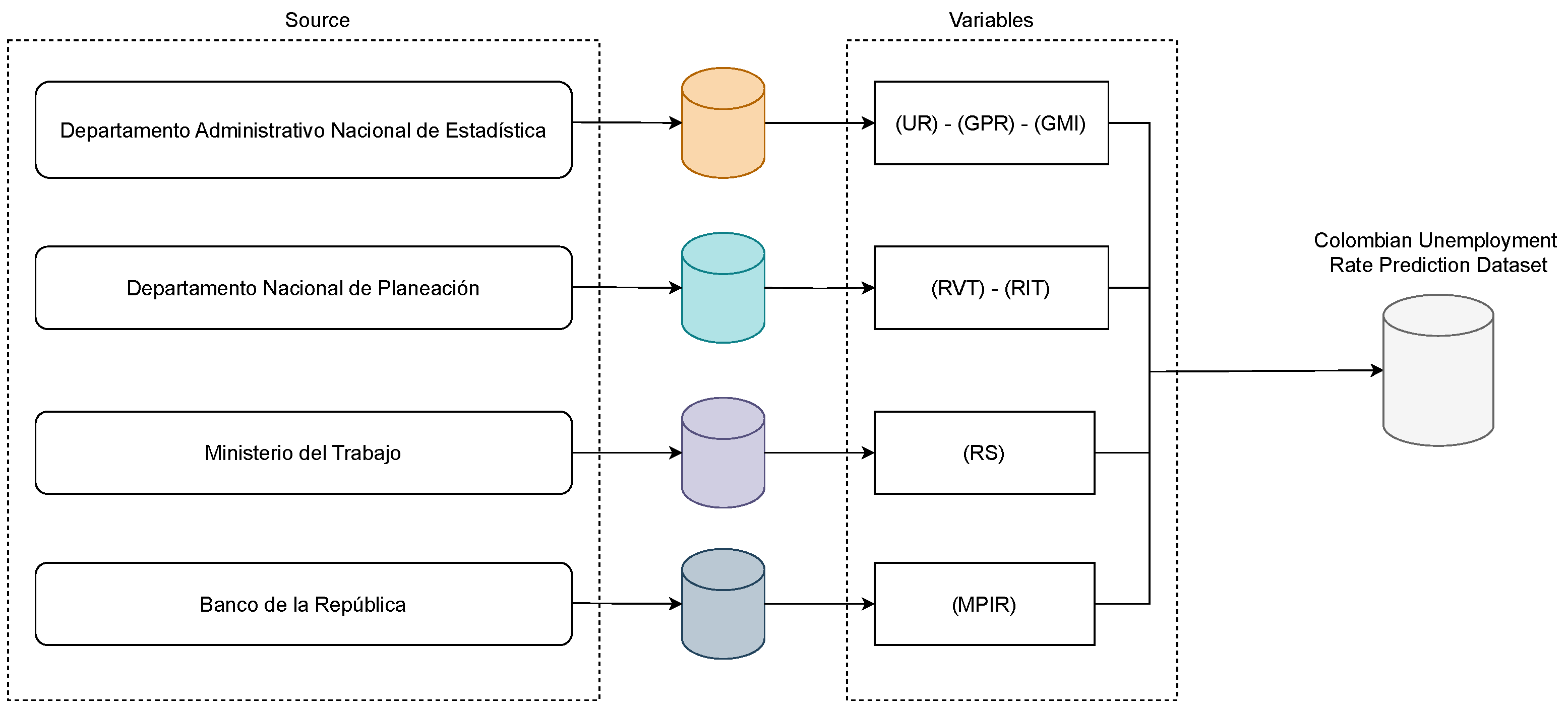
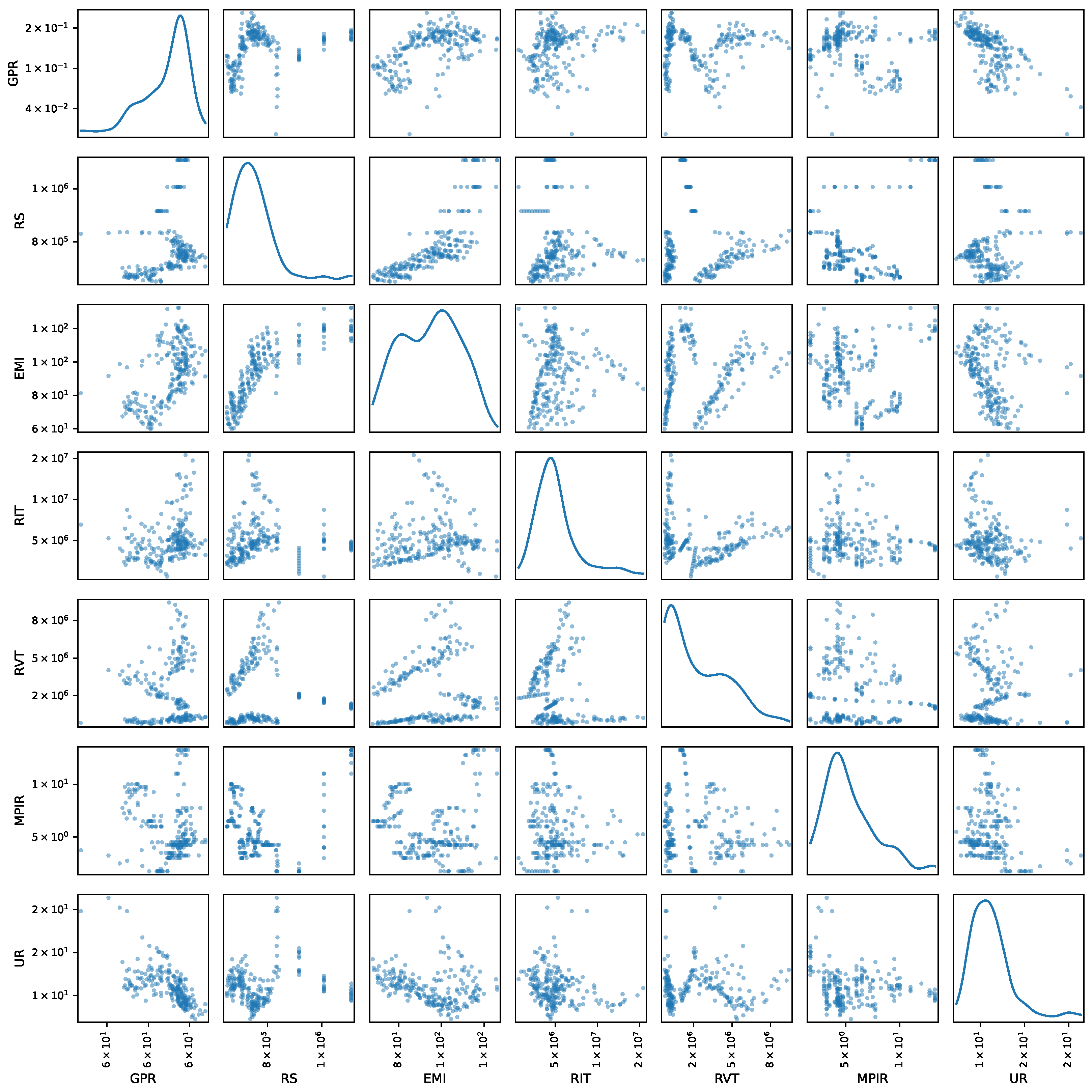
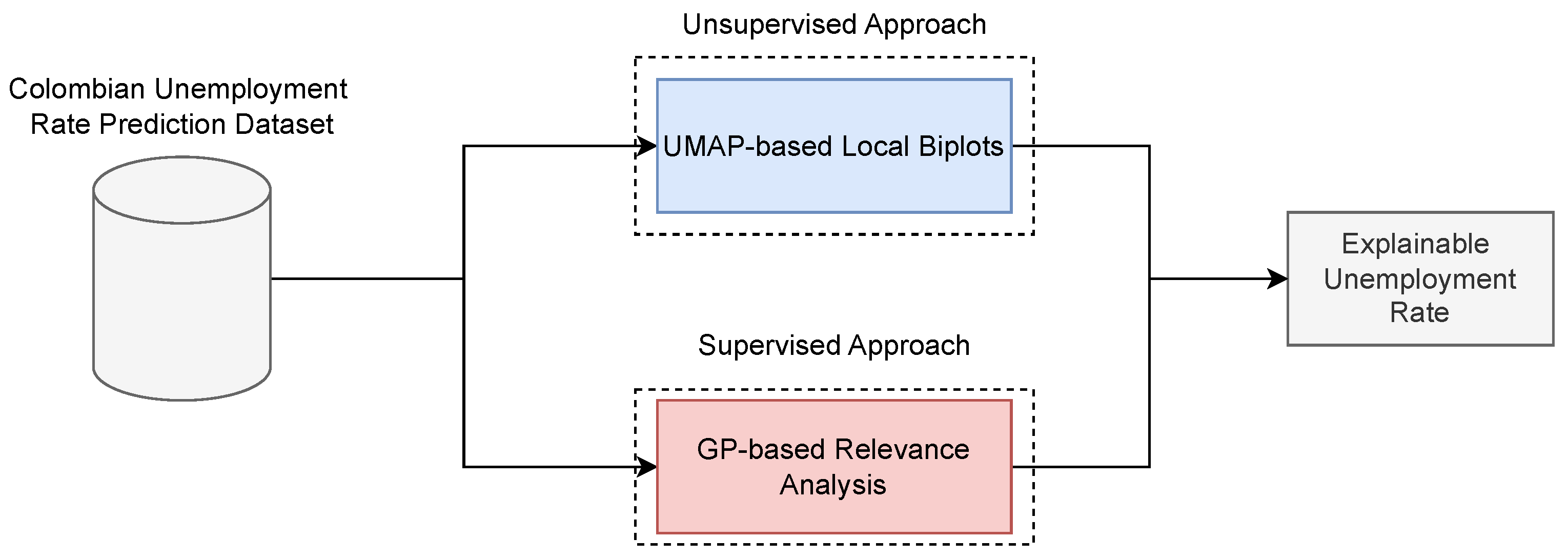
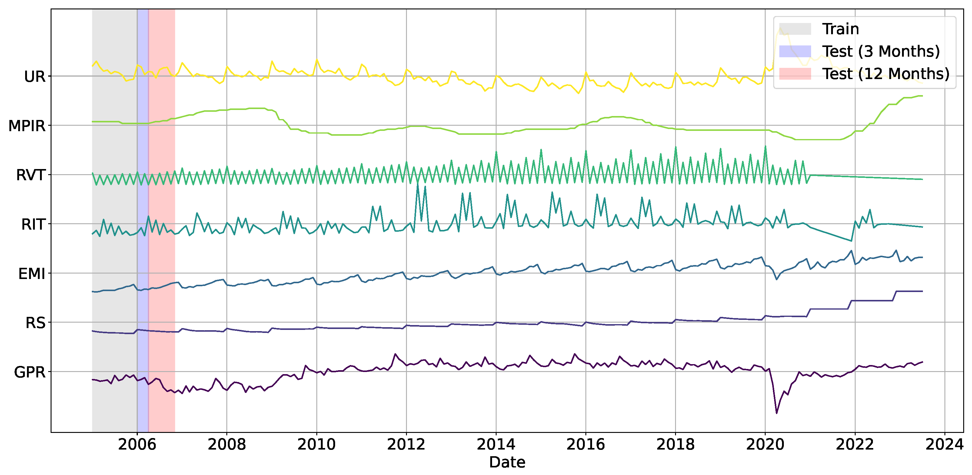


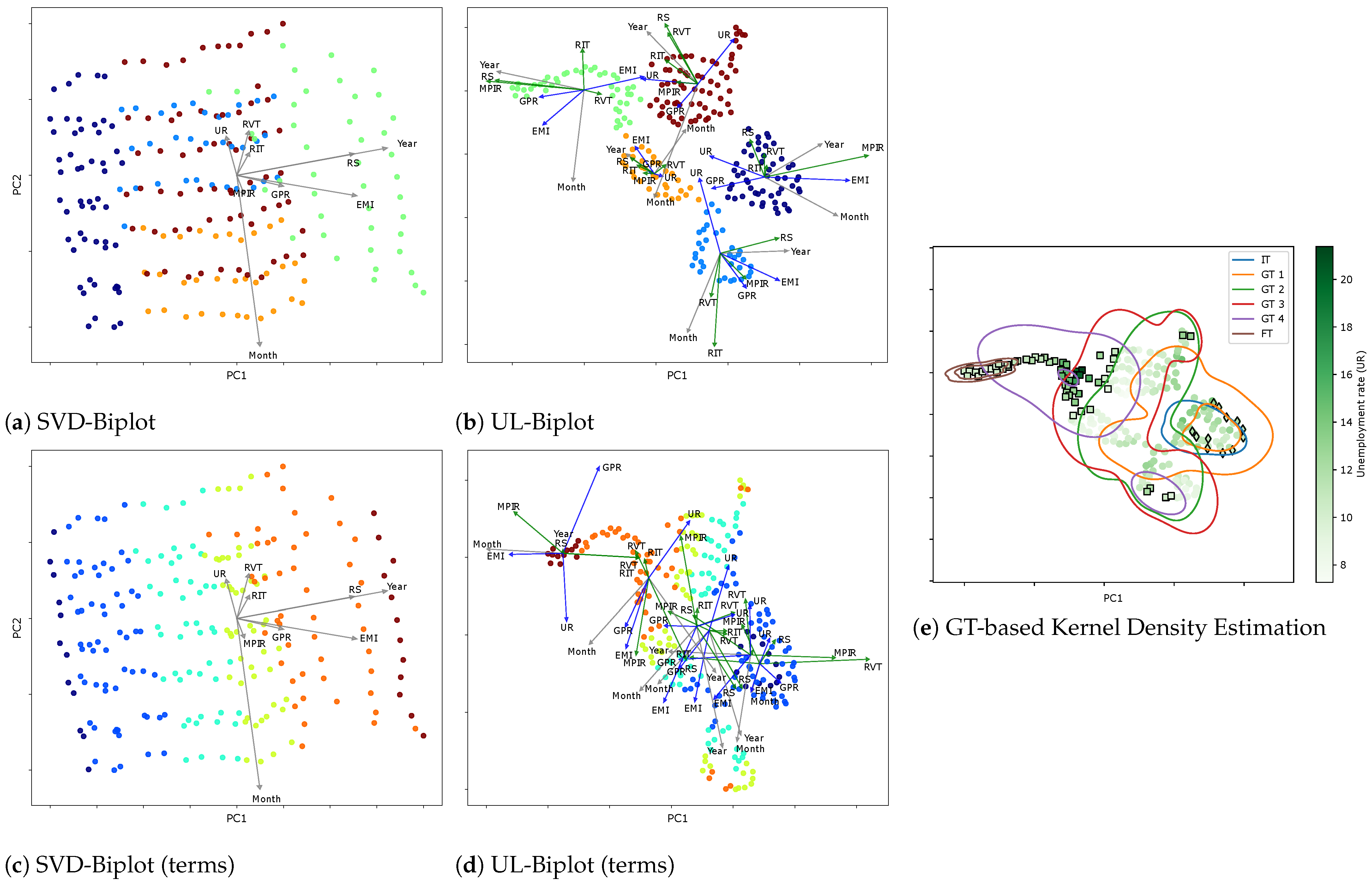
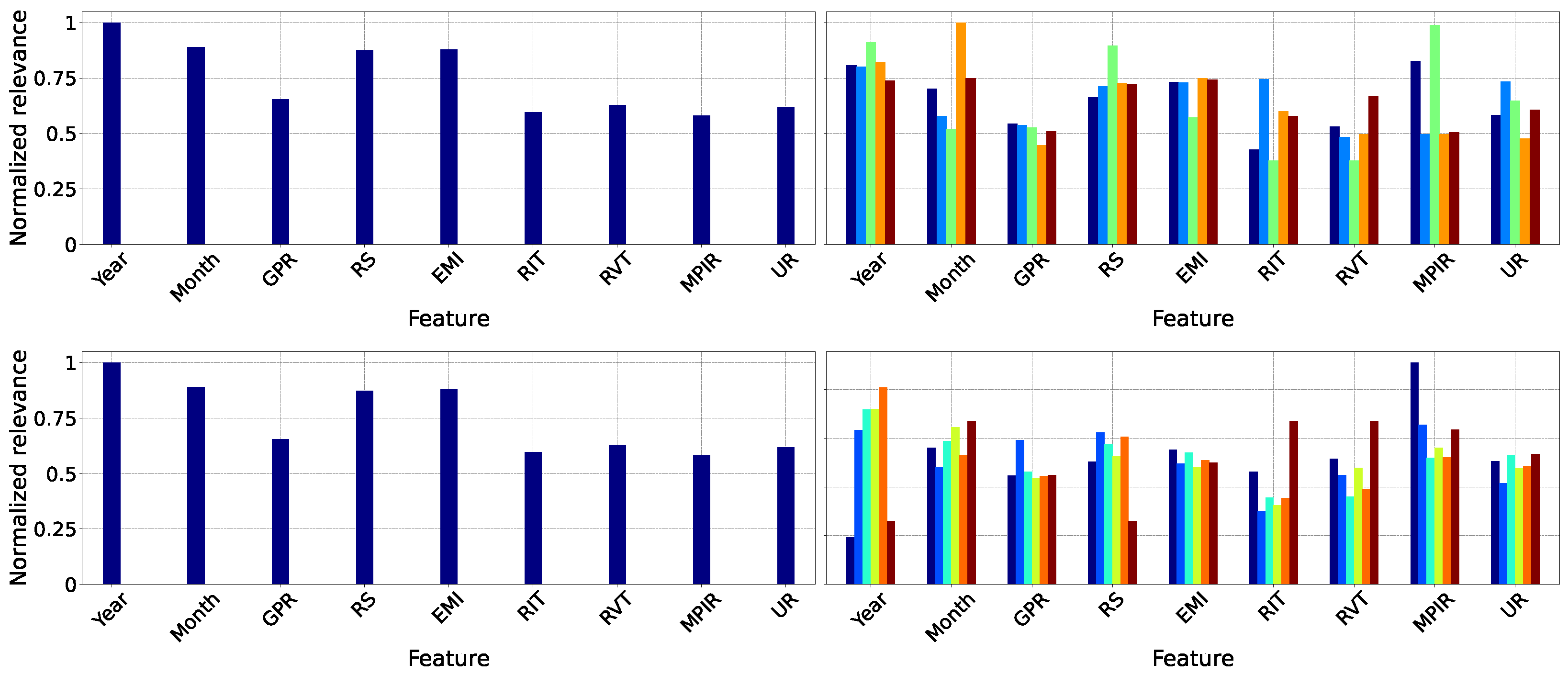
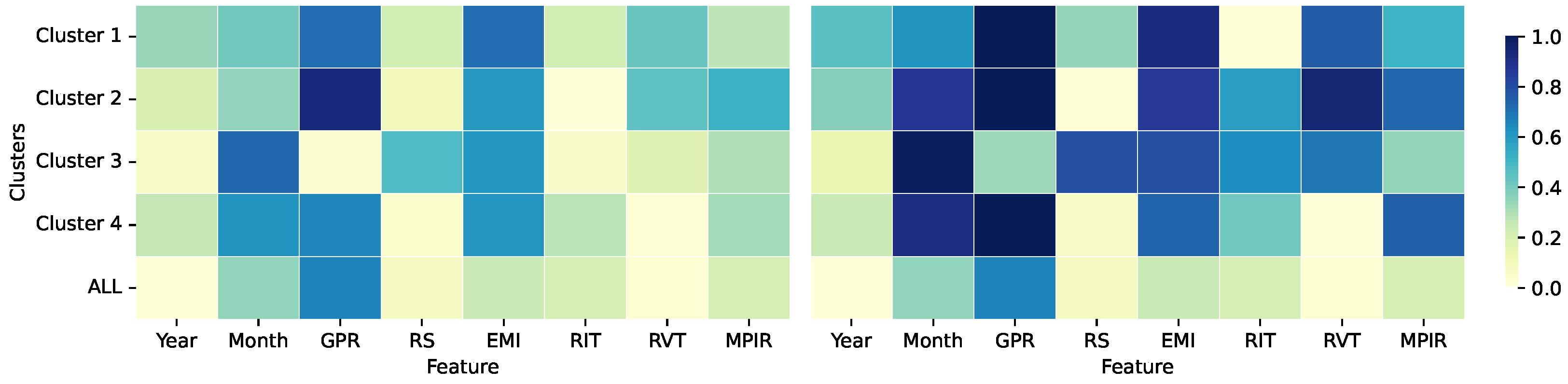
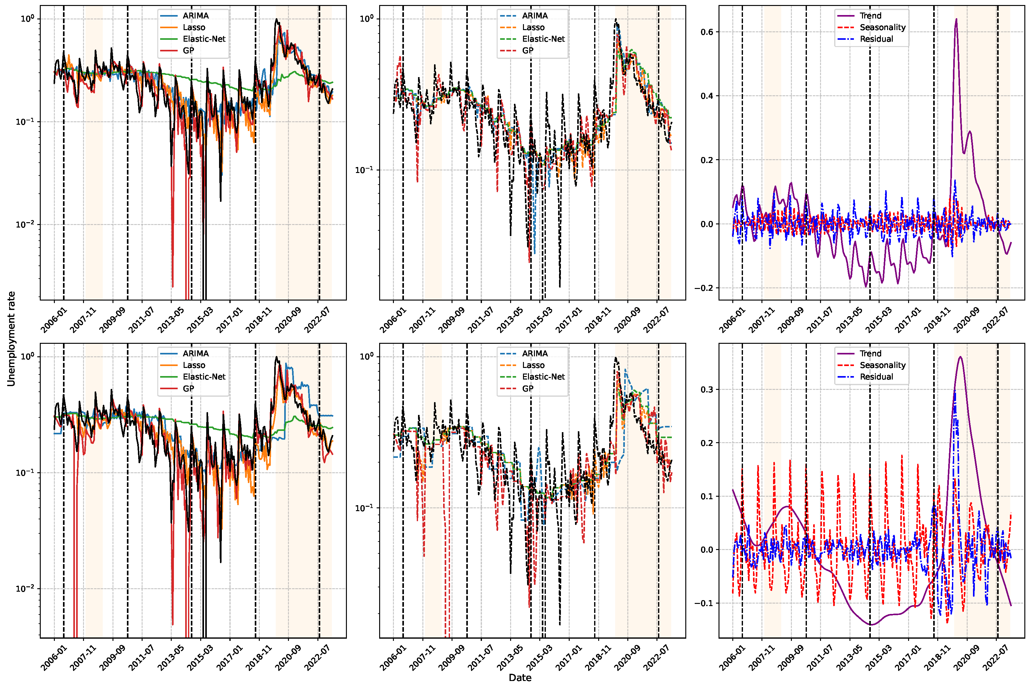
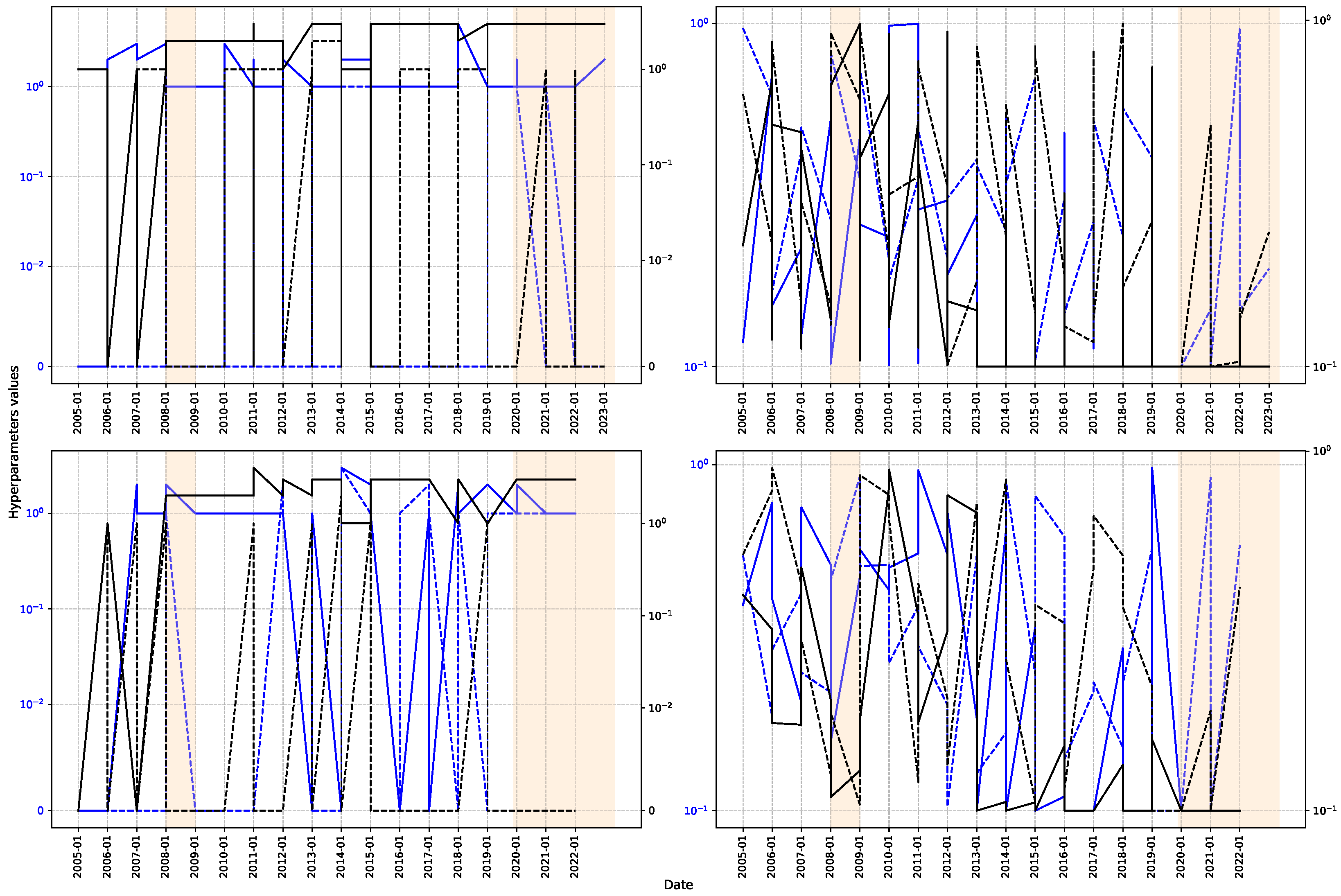
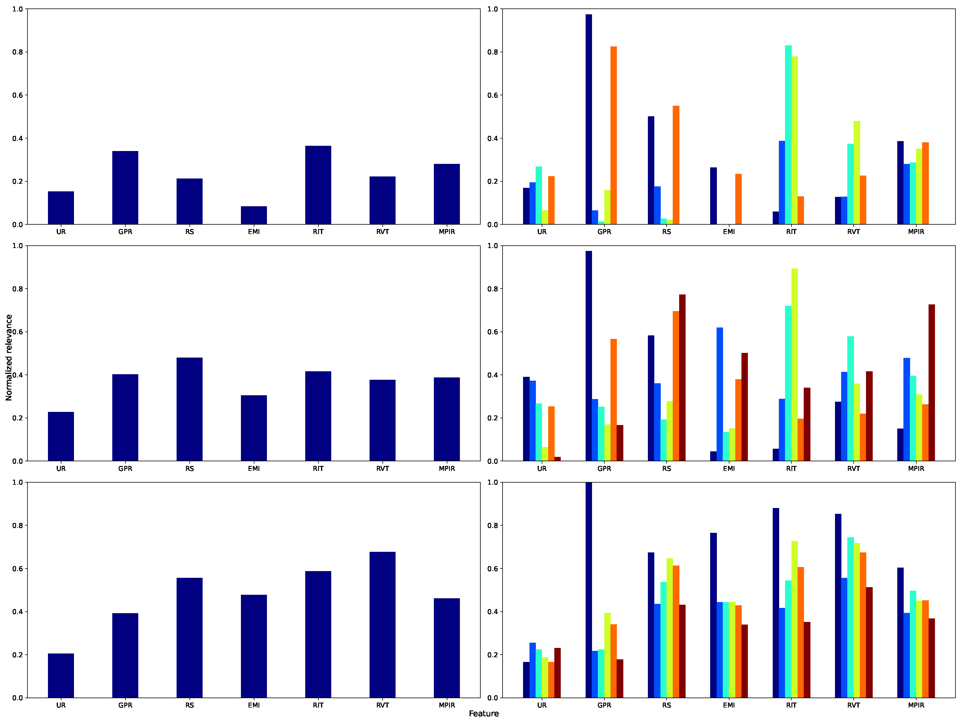

Disclaimer/Publisher’s Note: The statements, opinions and data contained in all publications are solely those of the individual author(s) and contributor(s) and not of MDPI and/or the editor(s). MDPI and/or the editor(s) disclaim responsibility for any injury to people or property resulting from any ideas, methods, instructions or products referred to in the content. |
© 2025 by the authors. Licensee MDPI, Basel, Switzerland. This article is an open access article distributed under the terms and conditions of the Creative Commons Attribution (CC BY) license (https://creativecommons.org/licenses/by/4.0/).