A Novel Methodology for Scrutinizing Periodic Solutions of Some Physical Highly Nonlinear Oscillators

Abstract

The study offers a comprehensive investigation of periodic solutions in highly nonlinear oscillator systems, employing advanced analytical and numerical techniques. The motivation stems from the urgent need to understand complex dynamical behaviors in physics and engineering, where traditional linear approximations fall short. This work precisely applies He’s Frequency Formula (HFF) to provide theoretical insights into certain classes of strongly nonlinear oscillators, as illustrated through five broad examples drawn from various scientific and engineering disciplines. Additionally, the novelty of the present work lies in reducing the required time compared to the classical perturbation techniques that are widely employed in this field. The proposed non-perturbative approach (NPA) effectively converts nonlinear ordinary differential equations (ODEs) into linear ones, equivalent to simple harmonic motion. This method yields a new frequency approximation that aligns closely with the numerical results, often outperforming existing approximation techniques in terms of accuracy. To aid readers, the NPA is thoroughly explained, and its theoretical predictions are validated through numerical simulations using Mathematica Software (MS). An excellent agreement between the theoretical and numerical responses highlights the robustness of this method. Furthermore, the NPA enables a detailed stability analysis, an area where traditional methods frequently underperform. Due to its flexibility and effectiveness, the NPA presents a powerful and efficient tool for analyzing highly nonlinear oscillators across various fields of engineering and applied science.

1. Introduction

An examination of historical and modern progress in the system identification of nonlinear dynamical structures was conducted [1]. The objective was to highlight various significant approaches found in the scientific community, so as to illustrate them through numerical and experimental applications in this field. Structures that exhibit either fundamental or complex geometric or material properties are subjected to varying levels of vibration from many sources, including earthquakes, wind loads, traffic movements, and imbalances in rotating machinery [2]. Excessive vibrations adversely affect the performance, integrity, and maintenance of structures, potentially leading to structural instability and breakdowns [3]. Structural damping is often a beneficial dynamic characteristic that reduces system vibrations to an acceptable threshold [4,5]. The research presented a method of calculating Coulomb and viscous friction coefficients using the replies of a harmonically excited dual-damped oscillator with linear stiffness. The identification method utilized established analytical solutions for non-sticking reactions induced near resonance, which were influenced by both internal and external factors, such as material degradation, geometric modifications, and boundary conditions [6]. Structural damping is often classified into three categories based on complex mechanics. First, damping originates from hydrodynamic or aerodynamic forces exerted on the structures [7]. Second, material damping originates from complex atomic and molecular interactions within materials [8]. Third, structural damping, resulting from Coulomb friction among components within a structural system, has been recognized [9]. A variety of simpler models have been suggested for damping characterization, including viscous damping and Coulomb frictional damping models [10]. The Mathieu–Duffing oscillator (DO) represents a fundamental model of a parametrically driven system distinguished by cubic nonlinearities. In multi-degree-of-freedom systems, parametric resonances and associated limit cycles manifest at both fundamental and combination resonance frequencies [11]. Moreover, the wideband instability of the simple solution and the creation of limit cycles of non-resonant frequencies were caused by the use of asynchronous parametric excitation of coupling terms.

The field of nonlinear oscillation in mathematics and engineering is becoming more and more significant and interesting. It is applied to engineering problems including materials, energy, and electrical infrastructure, as well as dynamical systems like networking mathematics and optimization [12,13]. Numerous analytical and numerical approaches are applied to solve such systems. The linked method computes higher-order approximations, performing exceptionally well across the whole range of beginning amplitudes. Consequently, novel frequency–amplitude connections have been found by applying the coupled homotopy-variational strategy to solve the nonlinear DO [14]. A system of this kind, comprising two springs—one linear and the other nonlinear—and a mass supported on them, was studied in [15]. Numerous researchers have focused their attention on several remarkable oscillators that have significant applications in engineering and physics. In order to provide an estimated analytical solution of the comprehensive ODE, the homotopy perturbation method (HPM) was performed [16]. Wang [17] proposed a new procedure based on the Rayleigh–Ritz method, and a newly proposed extended Galerkin method was analyzed in [18]. Consequently, various physically significant oscillators have been examined as special examples of this solution. Two strong linear terms were added to a nonlinear oscillator [19]. It was demonstrated that the HPM is a valuable mathematical tool for studying nonlinear oscillators, and this brief remark can serve as a model of numerous different applications that seek to determine the period or frequency of nonlinear oscillators [20]. One approximate analytical method used in studying strongly nonlinear dynamical systems was the Hamiltonian approach [21]. To discover an analytical solution to a nonlinear ODE with inertia and static nonlinearity, a unique technique that combines the HPM with a variational formula was developed [22]. The first-order approximation derived in this work was shown to be almost identical to exact solutions. In order to solve nonlinear third-order jerk ODEs, an adapted version of the comprehensive mistake minimization technique or global error minimization technique was anticipated [23]. To show the applicability and soundness of the approach, two instances were provided. The achieved analytical outcomes were compared and simulated with the exact numerical solution and known solutions.

An overview of amplitude–frequency equations of nonlinear oscillators was presented, accompanied by a proposed enhancement. Both the original and modified versions depend on the selected location, and thus far, no standardized criteria for site selection have been established [23]. A rapid prediction of the amplitude–frequency relationship of a nonlinear oscillator displaying discontinuity was essential [24]. The method yielded an estimated response with minimal processing and sufficient accuracy. A criterion for selecting a location point was presented in [25]. The DO was utilized to demonstrate the efficacy of the technique in [26]. The HFF originates from an ancient Chinese mathematical method and demonstrates an efficient strategy for tackling nonlinear oscillators. A different theoretical investigation of the formulation demonstrated its reliability and practicality in practical situations, where a modified version was proposed [27]. A formula linking the amplitude and period of an ODE was derived by comparing a nonlinear oscillator with its linear counterpart in a domain where oscillations were analyzed [28]. The amplitude–period formula relies on an integer, which can be ideally determined for specific instances; several examples are provided that contrast the approximation with the established HFF in [29]. The choice of an appropriate weight function in the objective functional leads to a definitive result, which has proven to be an excellent approximation of the exact time in numerous typical cases [30]. The HFF approach establishes the relationship between frequency and amplitude in a nonlinear oscillator when examining the residuals of two trial solutions. The calculation of the residuals can be further refined without sacrificing accuracy. The highly nonlinear DO was documented as a model to validate the solution’s methodology and precision [31]. The literature includes examples where the NPA was used to examine non-conservative oscillations, focusing on specific conditions and employing advanced methods for investigating a particular type of nonlinear vibration. The NPA operates independently, distinct from perturbation theory, which uses expansions to create polynomial approximations. While perturbation theory successfully provides initial series terms, the NPA can struggle with fundamental problem aspects. However, it intermittently utilizes approximate analytic continuation [32,33,34,35,36,37,38,39,40,41,42,43,44,45,46,47], transitioning from a polynomial approximation to the final NPA conclusion. This sophisticated technique moves beyond conventional constraints, enabling a more profound insight into complex challenges.

The investigation of periodic responses in highly nonlinear ODEs possesses considerable experimental and practical relevance across diverse scientific and technical fields. In experimental physics and engineering, comprehending periodic solutions is crucial for predicting and regulating the behavior of nonlinear mechanical systems, including pendulums with substantial amplitudes, vibrating beams, and intricate spring–mass systems, which are vital for structural health monitoring and mechanical resonance analysis. In electrical engineering, nonlinear oscillations occur in circuits containing diodes and transistors, where the analysis of periodic solutions facilitates the design of stable electronic oscillators, filters, and signal processing devices. The examination of periodic motions in nonlinear oscillators is essential in aerospace and mechanical engineering for maintaining the stability of aircraft wings, turbine blades, and rotating gear, thereby mitigating undesirable vibrations that may result in fatigue failure. Moreover, in materials science and nanotechnology, nonlinear oscillatory behavior is pertinent in atomic force microscopy, where careful regulation of oscillations is essential for high-resolution surface imaging. Biomechanical applications encompass the modeling of nonlinear oscillations in cardiovascular dynamics, cerebral activity, and human gait analysis, hence aiding in medical diagnostics and prosthetic creation. Moreover, geophysical applications encompass the examination of seismic wave propagation, whereby periodic solutions facilitate the comprehension of earthquake dynamics and the engineering of buildings capable of enduring seismic disturbances. The examination of periodic responses in plasma physics and fluid dynamics enhances the comprehension of wave propagation in plasmas and turbulent fluid flows, which is essential for progress in fusion energy research and aerodynamic design. Examining periodic solutions in highly nonlinear oscillations is essential for enhancing the effectiveness, safety, and productivity of diverse systems in science, engineering, and technology. Consequently, the following conclusions illustrate some advantages of the NPA:

• The suggested method is suitable for obtaining an accurate solution for extremely nonlinear oscillators.
• The proposed approach is less complicated and requires less processing and time than the classical perturbation techniques.
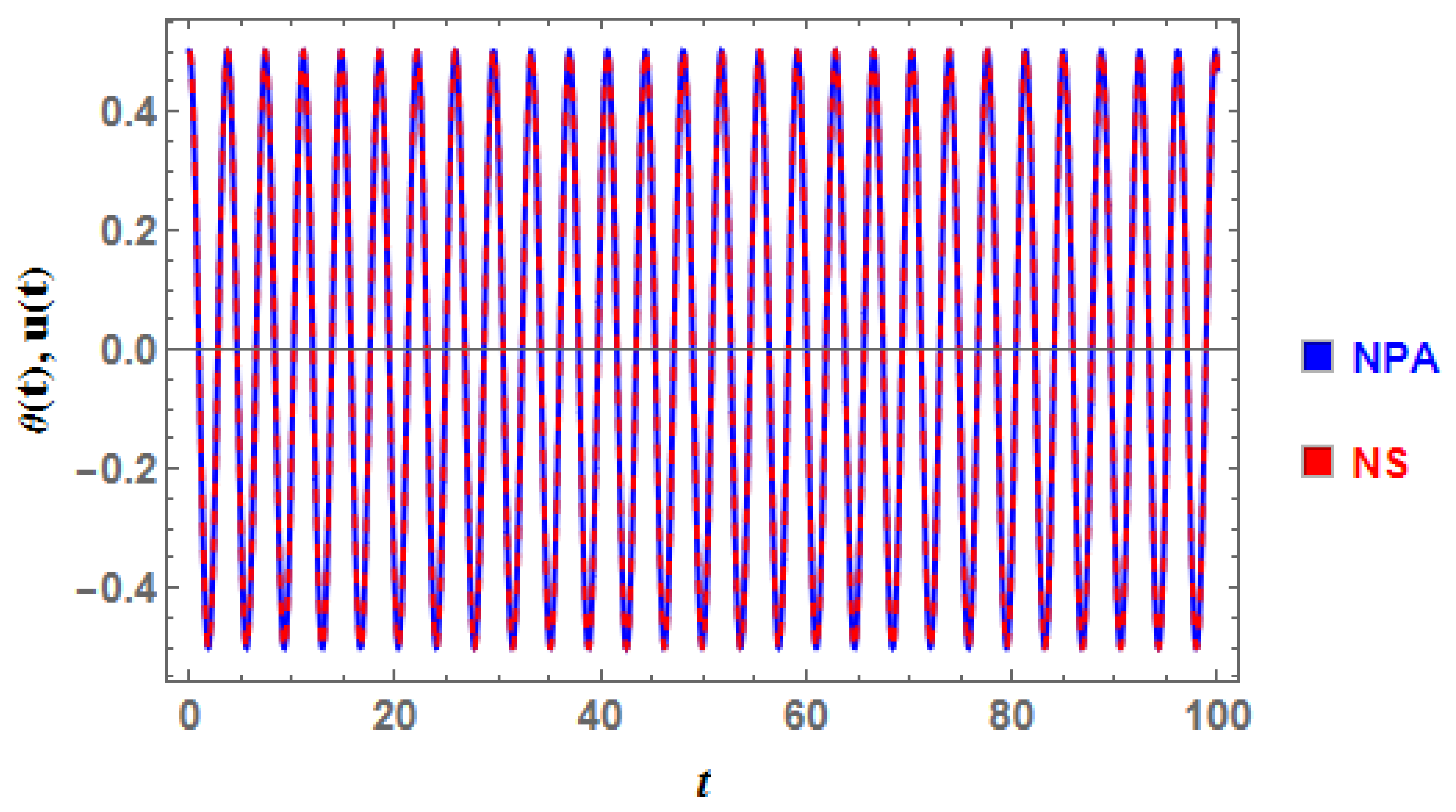
• The advantage of the NPA lies in its simplicity compared to other perturbation methods, and there is strong agreement with the numerical solutions.
• The disadvantage of the present technique is that as the amplitude $A$ values increase, the solution´s shape is farther away from the numerical solution’s shape

In order to clarify the performance of this paper, the rest of the article will be separated into the following sections to better explain how our investigation was carried out: The explanation of the NPA is offered in Section 2. Five different highly nonlinear ODEs are analyzed in Section 3. Lastly, our closing remarks are presented in Section 4.

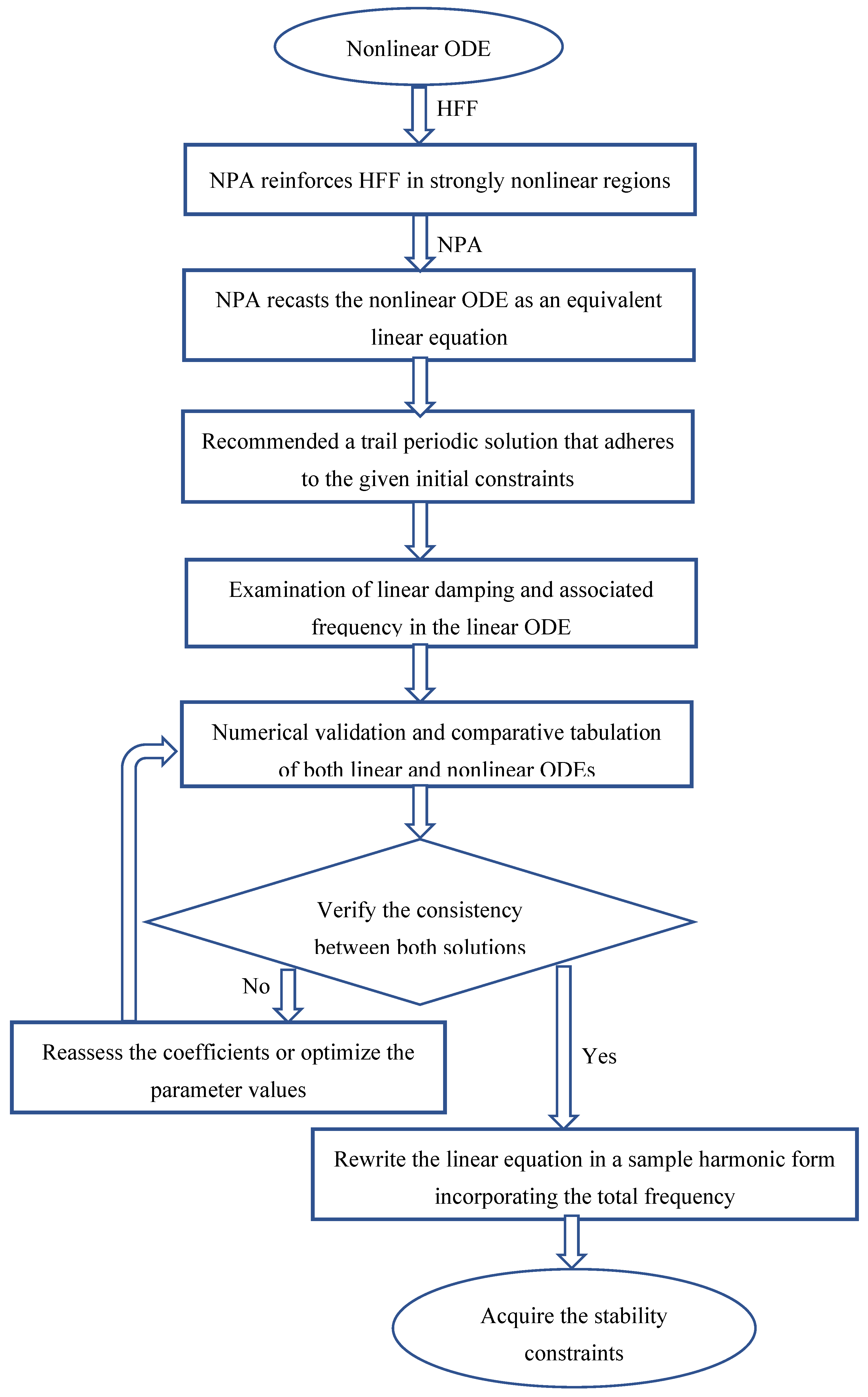
2. Description of the NPA

This section outlines the transformation of a nonlinear ODE into a linear ODE that has an exact solution. This linearization process´s major aspects are emphasized, demonstrating its feasibility and successful application to the novel organization, as previously described in [48]. Using the HFF method, a nonlinear oscillator is linearized, generating a linear counterpart whose solution accurately represents the entire oscillation period [49]. The existence and uniqueness of such a corresponding linear system are rigorously established [50]. The NPA is subsequently defined as follows:

In the context of a general nonlinear ODE, the nonlinear forces can be categorized into three distinct characteristics: quadratic nonlinear forces (which do not create secular terms), odd nonlinear damping forces (which produce secular terms), and restoring nonlinear odd forces (which also yield secular terms). Consequently, any nonlinear ODE can be restructured utilizing these components, as illustrated in the following example:

$$\ddot{u}+f(u,\hspace{0.17em}\dot{u},\hspace{0.17em}\ddot{u})+g(u,\hspace{0.17em}\dot{u},\hspace{0.17em}\ddot{u})+h(u,\hspace{0.17em}\dot{u},\hspace{0.17em}\ddot{u})=0,$$

(1)

where $f(u\hspace{0.17em}\dot{u},\ddot{u})$, $g(u\hspace{0.17em}\dot{u},\ddot{u})$, and $h(u\hspace{0.17em}\dot{u},\ddot{u})$ are the odd damping secular terms, even non-secular terms, and odd secular terms, respectively, in which they are defined as follows:

$$\left.\begin{array}{c}f(u,\hspace{0.17em}\dot{u},\hspace{0.17em}\ddot{u})=a_1\dot{u}+b_1{u}^2\dot{u}+c_{1}u{\dot{u}}^2+d_1{\dot{u}}^3+e_1\ddot{u}{\dot{u}}^2\\ g(u,\hspace{0.17em}\dot{u},\hspace{0.17em}\ddot{u})=a_2\dot{u}u+b_2{\dot{u}}^2+c_2{u}^2+d_2\dot{u}\ddot{u}\\ h(u,\hspace{0.17em}\dot{u},\hspace{0.17em}\ddot{u})={\omega }^{2}u+b_{3}u\dot{u}\ddot{u}+c_3{u}^2\dot{u}+d_3{u}^3+e_3\ddot{u}{u}^2\end{array}\right\},$$

(2)

where $\omega$ represents the natural frequency, while $a_j,\hspace{0.17em}{b}_j,\hspace{0.17em}{c}_j,\hspace{0.17em}{d}_j,\hspace{0.17em}\hspace{0.17em}\mathrm{and}\hspace{0.17em}\hspace{0.17em}{e}_j\hspace{0.17em}\hspace{0.17em}\hspace{0.17em}(j=1,\hspace{0.17em}2,3)$ are real constant physical coefficients.

The HFF seeks to transform the nonlinear ODE presented in Equation (1) into a linear one, as demonstrated by Moatimid et al. [32,33,34,35,36,37,38,39,40,41,42,43,44,45,46,47].

$$\ddot{u}+{\sigma }_{eqv}\dot{u}+{\omega }_{eqv}^{2}u=\lambda .$$

(3)

Equation (3) is a linear ODE that can be determined using conservative techniques. The goal is to calculate the coefficients contained in Equation (3). As can be seen, Equation (3) involves the damping constant ${\sigma }_{eqv}$ (equivalent damping), ${\omega }_{eqv}^2$ (equivalent frequency), and the non-homogeneous part $\lambda$. As a limitation of the NPA, a trial (guessing) solution is expressed as $\tilde{u}(t)=A\cos \mathsf{\Omega }t$, where $A$ is the initial amplitude, and the total frequency is shortened to $\mathsf{\Omega }$, which will be determined later. This frequency comes simply from the standard normal-form approach. This concept may be simply introduced as $u(t)=\tilde{u}(t)\hspace{0.17em}Exp(-{\sigma }_{eqv}t/2)$, where $f(t)$ is an unknown function to be determined. Therefore, Equation (3) is then used to produce the harmonic equation shown below:

$$\ddot{\tilde{u}}+{\mathsf{\Omega }}^2\tilde{u}=\lambda Exp({\sigma }_{eqv}t/2),$$

(4)

where ${\mathsf{\Omega }}^2={\omega }_{eqv}^2-{\displaystyle \frac{1}{4}}{\sigma }_{eqv}^2$ represents the total frequency of the system.

Equation (3) describes the linear simple harmonic oscillator. He [50] analyzed this system by integrating specific functional properties. The relevant initial conditions (ICs) are provided below:

$$\hspace{0.17em}\hspace{0.17em}\tilde{u}(0)=A, \hspace{0.17em}\hspace{0.17em}\hspace{0.17em}\mathrm{and}\hspace{0.17em}\hspace{0.17em}\dot{\tilde{u}}(0)=0.$$

(5)

According to Moatimid et al. [32,33,34,35,36,37,38,39,40,41,42,43,44,45,46,47], the three factors that appeared from Equation (3) can be written as follows:

• Equivalent frequency formula:

Employing the HFF to show helpful scheming frequencies for the developed generalized $h(u,\hspace{0.17em}\dot{u},\hspace{0.17em}\ddot{u})$. According to Moatimid et al. [32,33,34,35,36,37,38,39,40,41,42,43,44,45,46,47], the corresponding parameter may be determined as follows:

$${\omega }_{eqv}^2={\displaystyle \underset{0}{\overset{2\pi /\mathsf{\Omega }}{\int }}\tilde{u}h(\tilde{u},\hspace{0.17em}\dot{\tilde{u}},\hspace{0.17em}\ddot{\tilde{u}})}dt/{\displaystyle \underset{0}{\overset{2\pi /\mathsf{\Omega }}{\int }}{\tilde{u}}^{2}dt}.$$

(6)

• Equivalent damping formula:

One may estimate the frequency for a particular function $f(u,\hspace{0.17em}\dot{u},\stackrel{⃛}{u})$ using the HFF. As shown by Moatimid et al. [32,33,34,35,36,37,38,39,40,41,42,43,44,45,46,47], the corresponding damping term can be determined as follows:

$${\sigma }_{eqv}={\displaystyle \underset{0}{\overset{2\pi /\mathsf{\Omega }}{\int }}\dot{\tilde{u}}f(\tilde{u},\hspace{0.17em}\dot{\tilde{u}},\hspace{0.17em}\ddot{\tilde{u}})}dt/{\displaystyle \underset{0}{\overset{2\pi /\mathsf{\Omega }}{\int }}{\dot{\tilde{u}}}^{2}dt}$$

(7)

• Non-secular part:

It must be recognized that the quadratic formula applies to the non-secular component. Accordingly, the inhomogeneity can be calculated by substituting $u\to kA,\hspace{0.17em}\dot{u}\to kA\mathsf{\Omega },\hspace{0.17em}\hspace{0.17em}\mathrm{and}\hspace{0.17em}\hspace{0.17em}\ddot{u}\to kA{\mathsf{\Omega }}^2$ in the even non-secular function $g(u,\hspace{0.17em}\dot{u},\hspace{0.17em}\hspace{0.17em}\ddot{u})$. As previously shown [32,33,34,35,36,37,38,39,40,41,42,43,44,45,46,47], the factor $k$ is defined as $k=1/2\sqrt{n-r}$, where $n$ indicates the order of the system and $r$ signifies the degree of freedom of the system. Therefore, in the present case, $n=2$ and $r=1$, so the significance of $k$ becomes $k=1/2$.

To achieve this, the nonlinear Equation (1) is transformed into the linear Equation (3). The conventional normal version of Equation (3) may be used to estimate the stability requirements in a simpler manner, where the formulation determines the total frequency: ${\mathsf{\Omega }}^2={\omega }_{eqv}^2-{\sigma }^2/4$.

The requirements for stability are ${\mathsf{\Omega }}^2>0$ and ${\sigma }_{eqv}>0$. A flowchart illustrating the NPA is presented in Figure 1 for enhanced convenience.

3. Applications

The section is devoted to utilizing the NPA, as previously described, to analyze five different examples that represent highly nonlinear oscillators.

3.1. Example 1

In this subsection, we examine an interesting and significant prototype for manufacturing constructions with inertia and static nonlinearity. The vibration of an inextensible clamped free taper has previously been examined [51,52]. It should be mentioned that Ismail [21] used an analytical coupled homotopy-variational technique to analyze this topic previously. This problem´s governing equation can be represented as follows:

$$\ddot{x}+x+\alpha x^4\ddot{x}+2\alpha {\dot{x}}^2{x}^3+\beta x^5=0, \hspace{0.17em}\hspace{0.17em}x(0)=0, \hspace{0.17em}\hspace{0.17em}\dot{x}(0)=0,.$$

(8)

where $x$ refers to the displacement, the dot stands for the time derivative, and $\alpha$ and $\beta$ are physical real constant coefficients. Equation (8) may be rewritten as follows:

$$\ddot{x}+h(x,\hspace{0.17em}\dot{x},\hspace{0.17em}\ddot{x})=0,$$

(9)

where $h(x,\hspace{0.17em}\dot{x},\hspace{0.17em}\ddot{x})=x+\alpha x^4\ddot{x}+2\alpha {\dot{x}}^2{x}^3+\beta x^5$.

To perform the NPA for the considered issue, suppose that the trial solution is given by

$$\tilde{u}(t)=A\cos \mathsf{\Omega }t,$$

(10)

where $\mathsf{\Omega }$ is the total frequency, which will be determined later.

In the present example, there is no damping term. Therefore, there is no equivalent damping term in the equivalent linear ODE. Furthermore, there is no quadratic function in the nonlinear ODE; hence, the resultant linear ODE becomes a homogeneous one. Then, according to Equation (6), the equivalent frequency is

$${\omega }_{eqv}^2=1+{\displaystyle \frac{A^4}{8}}\left(5\beta -3\alpha {\mathsf{\Omega }}^2\right).$$

(11)

Substituting from Equation (10) into Equation (6), and after transformation, the total frequency $\mathsf{\Omega }$ is given as follows:

$$\hspace{0.17em}\hspace{0.17em}{\mathsf{\Omega }}^2={\displaystyle \frac{8+5\beta A^4}{8+3\alpha A^4}}.$$

(12)

It follows that the comparable linear ODE is given as follows:

$$\ddot{\tilde{u}}+{\mathsf{\Omega }}^2\tilde{u}=0.$$

(13)

Therefore, the solution to Equation (10) of the equivalent linear ODE is

$$\tilde{u}=A\cos \left(\sqrt{{\displaystyle \frac{8+5\beta A^4}{8+3\alpha A^4}}}t\right).$$

(14)

The stability creation requires

$${\displaystyle \frac{8+5\beta A^4}{8+3\alpha A^4}}>0.$$

(15)

It follows that for all positive parameters of $\alpha ,\hspace{0.17em}\hspace{0.17em}\mathrm{and}\hspace{0.17em}\hspace{0.17em}\beta$, the system is always stable.

In Figure 2, the numerical solution of the nonlinear equation as given in Equation (8), along with the comparable linear ones as shown in Equation (13), is plotted for $\alpha =1,\hspace{0.17em}\beta =2,\hspace{0.17em}\hspace{0.17em}\mathrm{and}\hspace{0.17em}\hspace{0.17em}\hspace{0.17em}A=0.5$. Specifically, the numeric solution is obtained by MS through the command NDSolve.

Figure 1. Outline of the methodology, with a particular emphasis on integrating the NPA and HFF.

Figure 1. Outline of the methodology, with a particular emphasis on integrating the NPA and HFF.

It should be mentioned that the initial amplitude selection limits the NPA. The absolute error between the two answers in this instance is 0.002360, according to the NPA. It should be emphasized that this new methodology enables us to address the stability condition, in contrast to conventional perturbation approaches. The absolute error between the approximate and real values is also displayed in

Table 1. Validation of the conjunction of the numerical and NPA solutions at $A=0.5$.

$$\mathit{t}$$	Nonlinear ODE	Linear ODE	Absolute Error
0	0.5	0.5	0
5	$\begin{array}{c}0.160568\end{array}$	$0.159955$	$0.000612854$
10	$\begin{array}{c}-0.398322\end{array}$	$-0.397658$	$0.000663983$
15	$\begin{array}{c}-0.415448\end{array}$	$\begin{array}{c}-0.414384\end{array}$	$0.00106407$
20	$0.132280$	$\begin{array}{c}0.132527\end{array}$	$\begin{array}{c}0.000246982\end{array}$
25	$0.499144$	$0.499177$	$0.000033874$
30	$\begin{array}{c}0.188299\end{array}$	$\begin{array}{c}0.186857\end{array}$	$\begin{array}{c}0.00144226\end{array}$
35	$-0.379792$	$-0.379623$	$0.000168973$
40	$-0.431115$	$-0.429747$	$\begin{array}{c}0.001367345\end{array}$
45	$\begin{array}{c}0.103535\end{array}$	$\begin{array}{c}0.104662\end{array}$	$\begin{array}{c}0.00112743\end{array}$
50	$\begin{array}{c}0.496577\end{array}$	$\begin{array}{c}0.496712\end{array}$	$\begin{array}{c}0.000135333\end{array}$

. This table demonstrates how little the two alternatives differ from one another.

3.2. Example 2

As previously mentioned [53,54], let us examine the free vibrations of a constrained symmetrical beam containing an intermediary lumped mass:

The governing equation of motion was previously determined as follows:

$$\ddot{x}+\lambda x+{\epsilon }_1{x}^2\ddot{x}+{\epsilon }_{1}x{\dot{x}}^2+{\epsilon }_2{x}^4\ddot{x}+2{\epsilon }_2{x}^3{\dot{x}}^2+{\epsilon }_3{x}^3+{\epsilon }_4{x}^5=0.$$

(16)

Equation (16) can be expressed in the same format as Equation (9), with $h(x,\hspace{0.17em}\dot{x},\hspace{0.17em}\ddot{x})=\lambda x+{\epsilon }_1{x}^2\ddot{x}+{\epsilon }_{1}x{\dot{x}}^2+{\epsilon }_2{x}^4\ddot{x}+2{\epsilon }_2{x}^3{\dot{x}}^2+{\epsilon }_3{x}^3+{\epsilon }_4{x}^5$. According to Equation (6), the equivalent frequency is

$${\omega }_{eqv}^2={\displaystyle \frac{1}{8}}\left(8\lambda +(6{\epsilon }_3-4{\epsilon }_1{\mathsf{\Omega }}^2)A^2+(5{\epsilon }_4-2{\epsilon }_2{\mathsf{\Omega }}^2)A^4\right).$$

(17)

The simplification of Equation (17) produces the following total frequency:

$${\mathsf{\Omega }}^2={\displaystyle \frac{8\lambda +6{\epsilon }_3{A}^2+5{\epsilon }_4{A}^4}{8+4{\epsilon }_1{A}^2+3{\epsilon }_2{A}^4}}$$

(18)

The corresponding linear ODE can be expressed as follows:

$$\ddot{\tilde{u}}+{\mathsf{\Omega }}^2\tilde{u}=0.$$

(19)

Consequently, the approximate linear solution to Equation (16) is

$$\tilde{u}=A\cos \left(\sqrt{{\displaystyle \frac{8\lambda +6{\epsilon }_3{A}^2+5{\epsilon }_4{A}^4}{8+4{\epsilon }_1{A}^2+3{\epsilon }_2{A}^4}}}t\right).$$

(20)

The stability criterion requires

$${\displaystyle \frac{8\lambda +6{\epsilon }_3{A}^2+5{\epsilon }_4{A}^4}{8+4{\epsilon }_1{A}^2+3{\epsilon }_2{A}^4}}>0,$$

(21)

and for all positive parameters of $\lambda ,\hspace{0.17em}\hspace{0.17em}{\epsilon }_1,\hspace{0.17em}\hspace{0.17em}{\epsilon }_2,\hspace{0.17em}\hspace{0.17em}{\epsilon }_3,\hspace{0.17em}\hspace{0.17em}{\epsilon }_4,\hspace{0.17em}\hspace{0.17em}\mathrm{and}\hspace{0.17em}\hspace{0.17em}\beta$, the system is always stable.

In Figure 3, the numerical solution of the nonlinear equation as given in Equation (16) is illustrated, along with the comparable linear ones as shown in Equation (19). For calculation, the following numeric data are applied:

$$\lambda =1,\hspace{0.17em}{\epsilon }_1=0.326845,\hspace{0.17em}{\epsilon }_2= 0.129579,\hspace{0.17em}{\epsilon }_3= 0.232598,\hspace{0.17em}{\epsilon }_4= 0.087584,\hspace{0.17em}\hspace{0.17em}\mathrm{and}\hspace{0.17em}A=0.5$$

Figure 2. The matching between the linear/nonlinear ODEs, as given in Equations (8) and (13), respectively.

Figure 2. The matching between the linear/nonlinear ODEs, as given in Equations (8) and (13), respectively.

Figure 3. Solutions of the linear/nonlinear ODEs, as presented in Equations (16) and (19), respectively.

Figure 3. Solutions of the linear/nonlinear ODEs, as presented in Equations (16) and (19), respectively.

Utilizing MS, the absolute error concerning the two solutions is specified as 0.005711.

The current technique demonstrates that the absolute error between the two responses is 0.005711. It is worth noting that, unlike classic perturbation techniques, the current NPA allows us to address the stability condition.

Table 2. Validation of the convergence of the real and NPA solutions at $A=0.1$.

$$\mathit{t}$$	Nonlinear ODE	Linear ODE	Absolute Error
0	0.1	0.1	0
5	0.0284085	0.0283927	$0.0000157697$
10	−0.0838879	−0.0838771	$\begin{array}{c}0.0000107690\end{array}$
15	−0.0760437	−0.0760227	$0.0000210166$
20	0.0407175	0.0407073	$\begin{array}{c}0.0000101092\end{array}$
25	0.099141	0.0991386	$0.0000023723$
30	0.0156095	0.0155889	$0.0000205708$
35	−0.090289	−0.0902865	$0.0000024933$
40	−0.0668907	−0.0668586	$0.0000321067$
45	0.0523244	0.0523207	$0.0000037713$
50	0.0965783	0.0965692	$0.0000090892$

also displays the absolute error between the actual and estimated outcomes. This table demonstrates that the differences between the two alternatives are minor.

3.3. Example 3

Let us consider a nano-resonator, which contains two stationary substrates and a moving electrode. The mobile electrode is positioned between two stationary electrodes, with a length of $l$, a width of $b$, and a thickness of $h$. It is defined within the coordinate system 0xyz, where $g_0$ represents the initial gap and $V$ denotes the electrostatic load [55,56,57,58]. Figure 4 shows a diagram illustration of a clamped–clamped resonator.

The equation of beam motion is formulated as follows:

$$\left(a_2-4a_4{u}^2+6a_6{u}^4-4a_8{u}^6+a_{10}{u}^8\right)\ddot{u}+K_{1}u+K_2{u}^3+K_3{u}^5+K_4{u}^7+K_5{u}^9+K_6{u}^{11}=0$$

(22)

where

$$\begin{array}{l}{K}_1=(1+\delta )b_1-{\chi }_{typ}N{c}_1-8{\alpha }_{Ca}{a}_2-6{\alpha }_{vdw}{a}_2-4\beta a_2-2\gamma \beta a_2,\\ K_2=-4(1+\delta )b_2+4{\chi }_{typ}N{c}_2-{\chi }_{typ}\alpha c_1{a}_0-8{\alpha }_{Ca}{a}_4+4{\alpha }_{vdw}{a}_4+8\beta a_4+6\gamma \beta a_4,\\ K_3=6(1+\delta )b_3-6{\chi }_{typ}N{c}_3+4{\chi }_{typ}\alpha c_2{a}_0+2{\alpha }_{vdw}{a}_6-4\beta a_6-6\gamma \beta a_6,\\ K_4=-4(1+\delta )b_4+4{\chi }_{typ}N{c}_4-6{\chi }_{typ}\alpha c_3{a}_0+2\gamma \beta a_8,\\ K_5=(1+\delta )b_5-{\chi }_{typ}N{c}_5+4{\chi }_{typ}\alpha c_4{a}_0,\\ K_6=-{\chi }_{typ}\alpha c_5{a}_0.\end{array}$$

$$\begin{array}{l}{a}_0={\int }_0^1{\phi }^{\prime 2}dx,\hspace{0.17em}\hspace{0.33em}\hspace{0.33em}\hspace{0.33em}{a}_1={\int }_0^1\phi dx,\hspace{0.17em}\hspace{0.33em}\hspace{0.33em}\hspace{0.33em}\hspace{0.33em}{a}_2={\int }_0^1{\phi }^{2}dx,\hspace{0.17em}\hspace{0.17em}\hspace{0.17em}\hspace{0.17em}{a}_3={\int }_0^1{\phi }^{3}dx,\hspace{0.17em}\hspace{0.33em}\hspace{0.33em}\hspace{0.33em}\hspace{0.33em}{a}_4={\int }_0^1{\phi }^{4}dx,\hspace{0.17em}\hspace{0.33em}\hspace{0.33em}\hspace{0.33em}{a}_5={\int }_0^1{\phi }^{5}dx,\\ a_6={\int }_0^1{\phi }^{6}dx,\hspace{0.17em}\hspace{0.33em}\hspace{0.33em}\hspace{0.33em}\hspace{0.33em}{a}_7={\int }_0^1{\phi }^{7}dx,\hspace{0.17em}\hspace{0.33em}\hspace{0.33em}\hspace{0.33em}{a}_8={\int }_0^1{\phi }^{8}dx, \hspace{0.17em}\hspace{0.17em}\hspace{0.17em}{a}_9={\int }_0^1{\phi }^{9}dx,\hspace{0.17em}\hspace{0.33em}\hspace{0.33em}\hspace{0.33em}\hspace{0.33em}{a}_{10}={\int }_0^1{\phi }^{10}dx.\end{array}$$

$$b_1={\int }_0^1\phi {\phi }^{(iv)}dx,\hspace{0.17em}\hspace{0.33em}{b}_2={\int }_0^1{\phi }^3{\phi }^{(iv)}dx,\hspace{0.17em}\hspace{0.33em}{b}_3={\int }_0^1{\phi }^5{\phi }^{(iv)}dx,b_4={\int }_0^1{\phi }^7{\phi }^{(iv)}dx,\hspace{0.17em}\hspace{0.33em}{b}_5={\int }_0^1{\phi }^9{\phi }^{(iv)}dx.$$

$$c_1={\int }_0^1\phi {\phi }^{″}dx,\hspace{0.17em}\hspace{0.33em}\hspace{0.33em}\hspace{0.33em}{c}_2={\int }_0^1{\phi }^3{\phi }^{″}dx,\hspace{0.17em}\hspace{0.33em}\hspace{0.33em}\hspace{0.33em}\hspace{0.33em}{c}_3={\int }_0^1{\phi }^5{\phi }^{″}dx,c_4={\int }_0^1{\phi }^7{\phi }^{″}dx,\hspace{0.17em}\hspace{0.33em}\hspace{0.33em}\hspace{0.33em}\hspace{0.33em}{c}_5={\int }_0^1{\phi }^9{\phi }^{″}dx.\hspace{0.33em}$$

The subsequent non-dimensional factors are used to regularize Equation (25), as shown in [59,60].

$$\begin{array}{c}w={\displaystyle \frac{\widehat{w}}{g}},\hspace{0.17em}\hspace{0.33em}\hspace{0.33em}x={\displaystyle \frac{X}{l}},\hspace{0.17em}\hspace{0.33em}\hspace{0.33em}\tau =t\sqrt{{\displaystyle \frac{\widehat{E}I}{\rho ph{l}^4}}},\hspace{0.17em}\hspace{0.33em}\hspace{0.33em}{\alpha }_{vdW}={\displaystyle \frac{ab{l}^4}{6\pi g_0^4\widehat{E}I}},\hspace{0.17em}{\alpha }_{C_a}={\displaystyle \frac{{\pi }^{2}hcb{l}^4}{240g_0^5\widehat{E}I}},\\ \delta ={\displaystyle \frac{\mu bh{\lambda }^2}{\widehat{E}I}},\hspace{0.17em} \hspace{0.17em}\gamma =0.65{\displaystyle \frac{g}{b}},\hspace{0.17em}\hspace{0.17em}\hspace{0.17em}\beta ={\displaystyle \frac{{\epsilon }_{0}b{V}^2{L}^4}{2g_0^3\widehat{E}I}},\hspace{0.17em}\hspace{0.17em}\hspace{0.17em}N={\displaystyle \frac{\widehat{N}{l}^2}{\widehat{E}I}},\hspace{0.17em}\hspace{0.33em}\hspace{0.33em}\hspace{0.33em}\alpha =6\left({\displaystyle \frac{g_0}{h}}\right).\end{array}$$

Equation (22) is rewritten in the form of Equation (9), where

$$h(u,\hspace{0.17em}\ddot{u})=-{\displaystyle \frac{4a_4}{a_2}}{u}^2\ddot{u}+{\displaystyle \frac{6a_6}{a_2}}{u}^4\ddot{u}-{\displaystyle \frac{4a_8}{a_2}}{u}^6\ddot{u}+{\displaystyle \frac{a_{10}}{a_2}}{u}^8\ddot{u}+{\displaystyle \frac{K_1}{a_2}}u+{\displaystyle \frac{K_2}{a_2}}{u}^3+{\displaystyle \frac{K_3}{a_2}}{u}^5+{\displaystyle \frac{K_4}{a_2}}{u}^7+{\displaystyle \frac{K_5}{a_2}}{u}^9+{\displaystyle \frac{K_6}{a_2}}{u}^{11}$$

Utilizing Formula (6) yields

$${\omega }_{eqv}^2={\displaystyle \frac{1}{512a_2}}\left(512K_1+A^2\left(\begin{array}{l}384K_2+231K_6{A}^8+1536a_4{\mathsf{\Omega }}^2+252A^6(K_5-a_{10}{\mathsf{\Omega }}^2)+\\ 320A^2(K_3-6a_6{\mathsf{\Omega }}^2)+280A^4(K_4+4a_8{\mathsf{\Omega }}^2)\end{array}\right)\right)$$

(23)

Substituting Equation (24) into Formula (6), with some modification, the total frequency is as follows:

$${\mathsf{\Omega }}^2={\displaystyle \frac{1}{512a_2}}\left(512K_1+A^2\left(\begin{array}{l}384K_2+231K_6{A}^8+1536a_4{\mathsf{\Omega }}^2+252A^6(K_5-a_{10}{\mathsf{\Omega }}^2)+\\ 320A^2(K_3-6a_6{\mathsf{\Omega }}^2)+280A^4(K_4+4a_8{\mathsf{\Omega }}^2)\end{array}\right)\right)$$

(24)

The simplification of Equation (24) produces

$${\mathsf{\Omega }}^2={\displaystyle \frac{512K_1+4A^4\left(96K_2+80A^2{K}_3+70A^4{K}_4+63A^6{K}_5\right)+231A^{10}{K}_6}{4\left(63A^8{a}_{10}+128a_2-384A^2{a}_4+480A^4{a}_6-280A^6{a}_8\right)}}.$$

(25)

The conforming linear ODE can be communicated as follows:

$$\ddot{x}+{\mathsf{\Omega }}^{2}x=0.$$

(26)

A microbeam that is electrostatically actuated is stable if it can remain in a steady condition when subjected to an electrostatic force. A fixed electrode and a voltage source create an electrostatic force, which pulls the microbeam in the opposite direction. The stability of a microbeam depends on how well its electrostatic force balances with its restorative mechanical force. To simplify the analysis, the correspondence between the original nonlinear ODE given in Equation (23) and the corresponding linear differential equation in Equation (26) is illustrated in Figure 5 for the selected system.

$$\begin{array}{l}{\mathrm{a}}_2=128/315, {\mathrm{a}}_4=32768/109395,\hspace{0.17em}{\mathrm{a}}_6= 4194304/16900975,\hspace{0.17em}{\mathrm{a}}_8=2147483648/9917826435,\hspace{0.17em}\\ {\mathrm{a}}_{10}=274877906944/1412926920405,\hspace{0.17em}{\mathrm{K}}_1=159.8984,\hspace{0.17em}{\mathrm{K}}_2=-300.468,\hspace{0.17em}{\mathrm{K}}_3=-932.565,\hspace{0.17em}\\ \hspace{0.17em}\hspace{0.17em}\hspace{0.17em}\hspace{0.17em}\hspace{0.17em}\hspace{0.17em}\hspace{0.17em}\hspace{0.17em}\hspace{0.17em}\hspace{0.17em}\hspace{0.17em}\hspace{0.17em}\hspace{0.17em}\hspace{0.17em}\hspace{0.17em}\hspace{0.17em}{\mathrm{K}}_4= 2602.52,\hspace{0.17em}{\mathrm{K}}_5=-1412.83,\hspace{0.17em}{\mathrm{K}}_6=353.732,\hspace{0.17em}\hspace{0.17em}\hspace{0.17em}\mathrm{and}\hspace{0.17em}\hspace{0.17em}\hspace{0.17em}\mathrm{A}=0.2\end{array}$$

The NS shows that the absolute error between the two solutions is 0.009507. It should be highlighted that, unlike classic perturbation approaches, the current NPA allows us to discuss the stability requirement.

3.4. Example 4

The motion $u(t)$ of a magnetic spherical pendulum is given as follows [61]:

$$\ddot{u}+\alpha \sin u-{\omega }^2\sin 2u=0,$$

(27)

where $\alpha ,\hspace{0.17em}\hspace{0.17em}\mathrm{and}\hspace{0.17em}\hspace{0.17em}\omega$ are two real physical quantities. In accordance with the NPA, Equation (27) can be rewritten in the form of Equation (9), where $h(u)=\alpha \sin u-{\omega }^2\sin 2u$. Following Formula (6) and integrating with the help of the MS, it is

$${\omega }_{eqv}^2={\displaystyle \frac{2}{A}}\left(\alpha J_1(A)-{\omega }^2{J}_1(2A)\right).$$

(28)

where $J_1$ is the Bessel function. Since there are no damping terms in the original nonlinear ODE, as given in Equation (27), it follows that the total frequency is equal to the equivalent frequency, and then the compatible linear ODE is given as follows:

$$\ddot{u}+{\mathsf{\Omega }}^{2}u=0.$$

(29)

The MS makes it easier to match the solution of the original nonlinear ODE (27) with the corresponding linear ODE for the selected sample system with numerical data: $\omega =0.1,\hspace{0.17em}\hspace{0.17em}\alpha =3.0,\hspace{0.17em}\hspace{0.17em}\mathrm{and}\hspace{0.17em}\hspace{0.17em}A=0.5$.

According to the NS, there is a 0.00233 absolute inaccuracy between the two responses as in Figure 6. It is worth noting that the current approach permits us to address the stability condition, as opposed to conventional perturbation techniques. For more convenience, in light of the total frequency as given in Equation (9) with Equation (28), the stability analysis can be displayed as follows:

In Figure 7, the stability profile for various values of the parameter $\omega$ are plotted. The parameter $\mathsf{\omega }$ plays a dual role in the stability profile of the system described by the equation $\ddot{u}+\alpha \sin u-{\omega }^2\sin 2u=0$. Firstly, it structurally alters the effective potential landscape by introducing a $\sin 2u$ component, which modulates the number and nature of equilibrium points, potentially creating multiple wells and barriers that affect where the system can settle. Secondly, $\omega$ functions dynamically as a bifurcation parameter, controlling the onset of instabilities or transitions between different motion regimes; as $\omega$ increases, it can sift stable points to unstable ones and trigger new oscillatory behaviors, thus playing a critical role in determining both the form and stability of solutions. Near the magnitude $A=1.9$ depicted in Figure 7, the parameter $\omega$ assumes a dual function in the stability profile. Physically, it adjusts the effective potential of the system by affecting the nonlinear term $u^2\sin u$, hence modifying the equilibrium point landscape and introducing various stability wells and barriers. Dynamically, it also serves as a bifurcation parameter; its fluctuation induces transitions between distinct oscillatory behaviors and stability regimes. As $\omega$ rises, these transitions may result in the development or dissolution of stable solutions, rendering $\omega$ essential in both defining the nature of solutions and regulating their stability in proximity to $A=1.9$.

Figure 6. NPA solution of the linear and NS solution of the nonlinear ODE (27) with the linear ODE (29), respectively.

Figure 6. NPA solution of the linear and NS solution of the nonlinear ODE (27) with the linear ODE (29), respectively.

In addition, the stability configuration depends on the parameter $\alpha$ (see Figure 8).

Figure 7. Stability profile for the linear ODE for various values of $\omega$.

Figure 7. Stability profile for the linear ODE for various values of $\omega$.

As shown in Figure 8, the parameter $\mathsf{\alpha }$ plays a destabilizing role in the stability profile by directly influening strength of the nonlinear restoring force through the $\sin \mathrm{u}$ term in the equation $\ddot{u}+\alpha \sin u-{\omega }^2\sin 2u=0$. As $\mathsf{\alpha }$ increases, it can amplify the force driving the system away from equilibrium, especially near $u=0$ and other critical points, thereby reducing the stability of fixed points or equilibria. In particular, a large $\alpha$ can steepen the potential energy landscape derived from the $\cos \mathrm{u}$ term, leading to sharper wells that may either trap the motion more tightly or, conversely, increase sensitivity to perturbations, potentially triggering bifurcations or chaotic behavior, depending on the interplay with $\omega$.

Figure 8. Impact of variations in parameter $\alpha$ on the stability diagram.

Figure 8. Impact of variations in parameter $\alpha$ on the stability diagram.

3.5. Example 5

Stringer-stiffened shells, commonly applied in ocean and aeronautical construction, are usually modeled as oscillatory systems. For mathematical description, the traditional shell theory, including Love´s first approximation for thin shells and the added stringers´ effects, is applied [62]. After undergoing certain mathematical transformations and making use of the assumption of the spatial distribution function, the mathematical model is obtained as follows:

$$\ddot{y}+\alpha y{\dot{y}}^2+\alpha y^2\ddot{y}+\beta y+\eta y^3+\lambda y^5=0,$$

(30)

where the coefficients in Equation (30) are real physical quantities. In light of the NPA, Equation (30) can be formulated as Equation (13), where $h(y,\hspace{0.17em}\dot{y},\hspace{0.17em}\ddot{y})=\alpha y{\dot{y}}^2+\alpha y^2\ddot{y}+\beta y+\eta y^3+\lambda y^5$. The integration in Equation (9) with the help of the MS produces the following:

Because the damping terms are disregarded, we have ${\mathsf{\Omega }}^2={\omega }_{eqv}^2$, where

$${\omega }_{eqv}^2={\displaystyle \frac{8\beta +6A^2\eta +5A^4\lambda }{4\left(2+A^2\alpha \right)}}.$$

(31)

Since there are no damping terms in the original nonlinear ODE given in Equation (30), it follows that the total frequency is the same as the equivalent frequency, and then the compatible linear ODE is given as follows:

$$\ddot{u}+{\mathsf{\Omega }}^{2}u=0.$$

(32)

The MS facilitates matching of the relevant linear ODE in Equation (32) for the chosen sample system with the original nonlinear ODE in Equation (30), which can be found in Figure 9 at

$$\beta =0.5,\hspace{0.17em}\hspace{0.17em}\alpha =3.0,\hspace{0.17em}\eta =0.3,\hspace{0.17em}\lambda =0.4,\hspace{0.17em}\hspace{0.17em}\mathrm{and}\hspace{0.17em}\hspace{0.17em}A=0.2$$

The NS claims that the two responses differ by 0.00469. Unlike conventional perturbation approaches, the current NPA allows us to tackle the stability criterion. For more convenience, as previously shown, the stability diagram for the variation in the parameter $\alpha$ is displayed in Figure 10. It can be seen that this parameter has a stabilizing influence on the stability profile. In order to keep a system in a stable and predictable state regardless of possible perturbations, this stabilizing impact is crucial.

The approximate solutions obtained using the NPA were compared to the numerical solutions using RK4 approximations, as shown in Figure 2, Figure 3, Figure 5, Figure 6 and Figure 9. The precisions of all generated analytical approximations utilizing the present approach and RK4 are extremely compatible. Given these comparisons, the present study introduces trust in the method utilized to locate a quick and effective analytical solution to the provided ODEs. Additionally, the proposed methodology demonstrates the potential for greater accuracy compared to conventional perturbation methods under certain conditions. The robust agreement between the analytical results obtained and the numerical approximations underscores the high precision achieved by the derived analytic solutions.

4. Concluding Remarks

The current study aimed to explore highly nonlinear oscillators in order to provide mathematical explanations for certain types of nonlinear ODE. For solving the nonlinear ODEs, we introduced the NPA, a simpler and more efficient alternative to classical perturbation methods. Unlike traditional techniques that rely on Taylor expansions, the NPA linearizes the nonlinear ODEs, producing a novel frequency analogous to simple harmonic motion. The NPA yields results that closely align with those of numerical simulations, particularly for physiologically relevant cases, and it surpasses standard methods in accuracy. Comparisons with the MS confirmed these findings. Crucially, the NPA enables detailed stability analysis and offers flexibility for addressing a wide range of nonlinear problems, making it valuable for both theoretical and applied research. However, its accuracy depends on small initial amplitudes and consistent initial conditions across examples.

Future research on periodic solutions in highly nonlinear multi-degree-of-freedom systems is essential for advancing both theoretical understanding and practical applications across the scientific and engineering domains. Enhancing current methods may lead to more accurate analytical and numerical tools for solving nonlinear ODEs and predicting system behavior under diverse conditions. Key directions include extending existing approaches to systems with time-dependent coefficients, external excitations, and complex, multi-degree-of-freedom interactions. Investigating stability and bifurcations can provide valuable insights into dynamic transitions that are critical for control and optimization in mechanical, aeronautical, and structural systems. Integrating machine learning and AI can improve solution accuracy and reduce computational costs, enabling real-time predictions. Experimental validation through advanced sensing and data acquisition will further strengthen models’ reliability. Exploring the effects of damping, driving forces, and parametric variations can deepen our understanding of real-world oscillatory systems, contributing to innovations in vibration control, energy harvesting, and precision engineering. Overall, this research is poised to bridge abstract mathematical theory with real-world applications in areas such as robotics, biomechanics, structural health monitoring, and nonlinear control. The ansatz for the eigenfunction yields accurate closed-form solutions to the relativistic Schrödinger equation, with a specified potential in both three and two dimensions, as previously presented [63]. The limitations on the parameters of the specified potential and the angular momentum quantum number were also delineated.

References

1. Kerschen, G.; Worden, K.; Vakakis, A.F.; Golinval Past, J.C. Present and future of nonlinear system identification in structural dynamics. Mech. Syst. Signal Process. 2006, 20, 505–592. [Google Scholar] [CrossRef]
2. Cao, M.S.; Sha, G.G.; Gao, Y.F.; Ostachowicz, W. Structural damage identification using damping: A compendium of uses and features. Smart Mater. Struct. 2017, 26, 043001. [Google Scholar] [CrossRef]
3. Blackwell, C.; Palazotto, A.; George, T.J.; Cross, C.J. The evaluation of the damping characteristics of a hard coating on titanium. Shock. Vib. 2007, 14, 37–51. [Google Scholar] [CrossRef]
4. Liang, J.W.; Feeny, B.F. Identifying Coulomb and viscous friction in forced dual-damped oscillators. J. Vib. Acoust. 2004, 126, 118–125. [Google Scholar] [CrossRef]
5. Mevada, H.; Patel, D. Experimental determination of structural damping of different materials. Process Eng. 2016, 144, 110–115. [Google Scholar] [CrossRef]
6. Zhang, X.; Du, X.; Brownjohn, J. Frequency modulated empirical mode decomposition method for the identification of instantaneous modal parameters of aero elastic systems. J. Wind Eng. Ind. Aerodyn. 2012, 101, 43–52. [Google Scholar] [CrossRef]
7. Kulkarni, P.; Bhattacharjee, A.; Nanda, B.K. Study of damping in composite beams. Mater. Today Proc. 2018, 5, 7061–7067. [Google Scholar] [CrossRef]
8. Chatterjee, A.; Chintha, H.P. Identification and parameter estimation of cubic nonlinear damping using harmonic probing and Volterra series. Int. J. Non-Linear Mech. 2020, 125, 103518. [Google Scholar] [CrossRef]
9. Dou, C.; Fan, J.; Li, C.; Cao, J.; Gao, M. On discontinuous dynamics of a class of friction-influenced oscillators with nonlinear damping under bilateral rigid constraints. Mech. Mach. Theory 2020, 147, 103750. [Google Scholar] [CrossRef]
10. Barakat, A.A.; Weig, E.M.; Hagedorn, P. Non-trivial solutions and their stability in a two-degree-of-freedom Mathieu–Duffing system. Nonlinear Dyn. 2023, 111, 22119–22136. [Google Scholar] [CrossRef]
11. Öcalan, Ö.; Özkan, U.M. Oscillations of dynamic equations on time scales with advanced arguments. Int. J. Dyn. Syst. Differ. Equ. 2016, 6, 275–284. [Google Scholar] [CrossRef]
12. Biçer, E.; Tunç, C. On the asymptotic stability behaviours of solutions of non-linear differential equations with multiple variable advanced arguments. J. Appl. Nonlinear Dyn. 2019, 8, 239–249. [Google Scholar] [CrossRef]
13. Ismail, G.M.; Abul-Ez, M.; Zayed, M.; Farea, N.M. Analytical accurate solutions of nonlinear oscillator systems via coupled homotopy-variational approach. Alex. Eng. J. 2022, 61, 5051–5058. [Google Scholar] [CrossRef]
14. Kopmaz, O. Free vibrations of a mass grounded by linear and non-linear springs in series. J. Sound Vib. 2006, 289, 689–710. [Google Scholar]
15. Manimegalai, K.; Sagar Zephania, C.F.; Bera, P.K.; Bera, P.; Das, S.K.; Sil, T. Study of strongly nonlinear oscillators using the Aboodh transform and the homotopy perturbation method. Eur. Phys. J. Plus 2019, 134, 462. [Google Scholar] [CrossRef]
16. Wang, J. The extended Rayleigh-Ritz method for an analysis of nonlinear vibrations. Mech. Adv. Mater. Struct. 2022, 29, 3281–3284. [Google Scholar] [CrossRef]
17. Shi, B.; Yang, J.; Wang, J. Forced vibration analysis of multi-degree-of-freedom nonlinear systems with the extended Galerkin method. Mech. Adv. Mater. Struct. 2023, 30, 794–802. [Google Scholar] [CrossRef]
18. Abu-As’ad, A.; Asad, J. Power series approach to nonlinear oscillators. J. Low Freq. Noise Vib. Act. Control 2024, 43, 220–238. [Google Scholar] [CrossRef]
19. Shou, D.-H. The homotopy perturbation method for nonlinear oscillators. Comput. Math. Appl. 2009, 58, 2456–2459. [Google Scholar] [CrossRef]
20. Hermann, M.; Saravi, M.; Khah, H.E. Analytical study of nonlinear oscillatory systems using the Hamiltonian approach technique. J. Theor. Appl. Phys. 2014, 8, 133. [Google Scholar] [CrossRef]
21. Ismail, G.M. An analytical coupled homotopy-variational approach for solving strongly nonlinear differential equation. J. Egypt. Math. Soc. 2017, 25, 434–437. [Google Scholar] [CrossRef]
22. Ismail, G.M.; Abu-Zinadah, H. Analytic approximations to non-linear third order jerk equations via modified global error minimization method. J. King Saud Univ.-Sci. 2021, 33, 101219. [Google Scholar] [CrossRef]
23. He, J.-H. Comment on He’s frequency formulation for nonlinear oscillators. Int. J. Nonlinear Sci. Numer. Simul. 2008, 29, 19–22. [Google Scholar] [CrossRef]
24. He, J.-H. An approximate amplitude-frequency relationship for a nonlinear oscillator with discontinuity. Nonlinear Sci. Lett. A 2016, 7, 77–85. [Google Scholar]
25. He, J.-H. Amplitude-frequency relationship for conservative nonlinear oscillators with odd nonlinearities. Int. J. Appl. Comput. Math. 2017, 3, 1557–1560. [Google Scholar] [CrossRef]
26. Ren, Z.-F. He’s frequency-amplitude formulation for nonlinear oscillators. Int. J. Mod. Phys. B 2011, 25, 2379–2382. [Google Scholar] [CrossRef]
27. Ren, Z.-F. Theoretical basis of He’s frequency-amplitude formulation for nonlinear oscillators. Nonlinear Sci. Lett. A 2018, 9, 86–90. [Google Scholar]
28. Garcıa, A. An amplitude-period formula for a second order nonlinear oscillator. Nonlinear Sci. Lett. A 2017, 8, 340–347. [Google Scholar]
29. Antola, R.S. Remarks on an approximate formula for the period of conservative oscillations in nonlinear second order ordinary differential equations. Nonlinear Sci. Lett. A 2017, 8, 348–351. [Google Scholar]
30. Younesian, D.; Askari, H.; Saadatnia, Z.; Yazdi, M.K. Frequency analysis of strongly nonlinear generalized Duffing oscillators using He’s frequency-amplitude formulation and He’s energy balance method. Comput. Math. Appl. 2010, 59, 3222–3228. [Google Scholar]
31. Ren, Z.-F.; Hu, G.-F. He’s frequency-amplitude formulation with average residuals for nonlinear oscillators. J. Low Freq. Noise Vib. Act. Control 2019, 38, 1050–1059. [Google Scholar] [CrossRef]
32. Ismail, G.M.; Moatimid, G.M.; Yamani, M.I. Periodic solutions of strongly nonlinear oscillators using He’s frequency formulation. Eur. J. Pure Appl. Math. 2024, 17, 2154–2171. [Google Scholar] [CrossRef]
33. Moatimid, G.M.; Amer, T.S. Dynamical system of a time-delayed ϕ6-Van der Pole oscillator: A non-perturbative approach. Sci. Rep. 2023, 13, 11942. [Google Scholar] [CrossRef]
34. Moatimid, G.M.; Amer, T.S.; Ellabban, Y.Y. A novel methodology for a time-delayed controller to prevent nonlinear system oscillations. J. Low Freq. Noise Vib. Act. Control 2024, 43, 525–542. [Google Scholar] [CrossRef]
35. Moatimid, G.M.; Amer, T.S.; Galal, A.A. Studying highly nonlinear oscillators using the non-perturbative methodology. Sci. Rep. 2023, 13, 20288. [Google Scholar] [CrossRef] [PubMed]
36. Moatimid, G.M.; El-Sayed, A.T.; Salman, H.F. Different controllers for suppressing oscillations of a hybrid oscillator via non-perturbative analysis. Sci. Rep. 2024, 14, 307. [Google Scholar] [CrossRef]
37. Alluhydan, K.; Moatimid, G.M.; Amer, T.S. The non-perturbative approach in examining the motion of a simple pendulum associated with a rolling wheel with a time-delay. Eur. J. Pure Appl. Math. 2024, 17, 3185–3208. [Google Scholar] [CrossRef]
38. Alluhydan, K.; Moatimid, G.M.; Amer, T.S.; Galal, A. A novel inspection of a time-delayed rolling of a rigid rod. Eur. J. Pure Appl. Math. 2024, 17, 2878–2895. [Google Scholar]
39. Alluhydan, K.; Moatimid, G.M.; Amer, T.S.; Galal, A.A. Inspection of a time-delayed excited damping Duffing oscillator. Axioms 2024, 13, 416. [Google Scholar] [CrossRef]
40. Ismail, G.M.; Moatimid, G.M.; Alraddadi, I.; Stylianos, V.; Kontomaris, S.V. Scrutinizing highly nonlinear oscillators using He’s frequency formula. Sound Vib. 2025, 59, 2358. [Google Scholar] [CrossRef]
41. Moatimid, G.M.; Amer, T.S.; Galal, A.A. Inspection of some extremely nonlinear oscillators using an inventive approach. J. Vib. Eng. Technol. 2024, 12, 1211–1221. [Google Scholar] [CrossRef]
42. Moatimid, G.M.; Mohamed, M.A.A.; Elagamy, K.H. Insightful examination of some nonlinear classification linked with Mathieu oscillators. J. Vib. Eng. Technol. 2025, 13, 173. [Google Scholar] [CrossRef]
43. Alanazy, A.; Moatimid, G.M.; Amer, T.S.; Mohamed, M.A.A.; Abohamer, M.K. A novel procedure in scrutinizing a cantilever beam with tip mass: Analytic and bifurcation. Axioms 2025, 14, 16. [Google Scholar] [CrossRef]
44. Moatimid, G.M.; Mohamed, M.A.A.; Elagamy, K.H. An innovative approach in inspecting a damped Mathieu cubic–quintic Duffing oscillator. J. Vib. Eng. Technol. 2024, 12 (Suppl. S2), S1831–S1848. [Google Scholar] [CrossRef]
45. Moatimid, G.M.; Mohamed, M.Y. Nonlinear electro-rheological instability of two moving cylindrical fluids: An innovative approach. Phys. Fluids 2024, 36. [Google Scholar] [CrossRef]
46. Alanazy, A.; Moatimid, G.M.; Mohamed, M.A.A. Innovative methodology in scrutinizing nonlinear rolling ship in longitudinal waves. Ocean Eng. 2025, 327, 120924. [Google Scholar] [CrossRef]
47. Moatimid, G.M.; El-Bassiouny, A.F.; Mohamed, M.A.A. Novel approach in inspecting nonlinear rolling ship in longitudinal waves. Ocean Eng. 2025, 327, 120975. [Google Scholar] [CrossRef]
48. Caughey, T.K. Equivalent linearization techniques. J. Acoust. Soc. Am. 1963, 35, 1706–1711. [Google Scholar] [CrossRef]
49. Spanos, P.-T.D.; Iwan, W.D. On the existence and uniqueness of solutions generated by equivalent linearization. Int. J. Non-Linear Mech. 1979, 13, 71–78. [Google Scholar] [CrossRef]
50. He, J.-H. Special functions for solving nonlinear differential equations. Int. J. Appl. Comput. Math. 2021, 7, 84. [Google Scholar] [CrossRef]
51. Farea, N.M.; Ismail, G.M. Analytical solution for strongly nonlinear vibration of a stringer shell. J. Low Freq. Noise Vib. Act. Control. 2025, 44, 81–87. [Google Scholar] [CrossRef]
52. Molla, M.H.U.; Razzak, M.A.; Alam, M.S. Harmonic balance method for solving a large-amplitude oscillation of a conservative system with inertia and static non-linearity. Results Phys. 2016, 6, 238–242. [Google Scholar] [CrossRef]
53. Hamdan, M.N.; Shabaneh, H. On the large amplitude free vibrations of restrained uniform beam carring an intermediate lumped mass. J. Sound Vib. 1997, 199, 711–835. [Google Scholar] [CrossRef]
54. Sfahani, M.G.; Barari, A.; Ganji, S.S.; Domairry, G.; Rokni, H.B. Dynamic response of a beam carrying a lumped mass along its span. Int. J. Adv. Manuf. Technol. 2013, 64, 1435–1443. [Google Scholar] [CrossRef]
55. Cveticanin, L.; Ismail, G.M. Higher-order approximate periodic solution for the oscillator with strong nonlinearity of polynomial type. Eur. Phys. J. Plus 2019, 134, 266. [Google Scholar] [CrossRef]
56. Ismail, G.M.; Hosen, M.A.; Mohammadian, M.; El-Moshneb, M.M.; Bayat, M. Nonlinear Vibration of Electrostatically Actuated Microbeam. Mathematics 2022, 10, 4762. [Google Scholar] [CrossRef]
57. Bayat, M.; Bayat, M.; Pakar, I. Nonlinear vibration of an electrostatically actuated microbeam. Lat. Am. J. Solids Struct. 2014, 11, 534–544. [Google Scholar] [CrossRef]
58. Fu, Y.; Zhang, J.; Wan, L. Application of the energy balance method to a nonlinear oscillator arising in the microelectromechanical system (MEMS). Curr. Appl. Phys. 2011, 11, 482–485. [Google Scholar] [CrossRef]
59. Ghalambaz, M.; Ghalambaz, M.; Edalatifar, M. Nonlinear oscillation of nanoelectro-mechanical resonators using energy balance method: Considering the size effect and the van der Waals force. Appl. Nanosci. 2016, 6, 309–317. [Google Scholar] [CrossRef]
60. Ismail, G.M.; Abul-Ez, M.; Farea, N.M.; Saad, N. Analytical approximations to nonlinear oscillation of nanoelectro-mechanical resonators. Eur. Phys. J. Plus 2019, 134, 47. [Google Scholar] [CrossRef]
61. Moatimid, G.M.; Amer, T.S. Analytical approximate solutions of a magnetic spherical pendulum: Stability analysis. J. Vib. Eng. Technol. 2023, 11, 2155–2165. [Google Scholar] [CrossRef]
62. Amabili, M. Comparison of shell theories for large-amplitude vibrations of circular cylindrical shells: Lagrangian approach. J. Sound Vib. 2003, 264, 1091–1125. [Google Scholar] [CrossRef]
63. Dong, S.-H. A new approach to the relativistic Schrödinger equation with central potential: Ansatz method. Int. J. Theor. Phys. 2001, 40, 559–567. [Google Scholar] [CrossRef]
Figure 4. Geometry for an electrostatically actuated micro-beam.
Computation 13 00105 g004
Figure 5. Solutions of the nonlinear/linear ODEs described in Equations (22) and (26), respectively.
Computation 13 00105 g005
Figure 9. Illustration of the link between the nonlinear and linear ODEs given in Equations (30) and (32), respectively.
Computation 13 00105 g009
Figure 10. The effect of the deviation in parameter α on the stability diagram.
Computation 13 00105 g010