State Observer for Deflections in Rectangular Flat Plates Simply Supported Subjected to Uniform and Hydrostatic Pressure

Abstract

The present work aims to validate the computational simulation model that determines the static deflection experienced by rectangular flat plates along the longest edge when subjected to uniform and hydrostatic pressures, proposed as a state observer for active control. The plates are isotropic and simply supported on their four edges. The pressures do not exceed the plate material’s elastic limit. The solutions in the analytical form of the partial differential equation of flat plates established by Kirchoff theory are first determined by Fourier double series. On the other hand, simulations are performed using the Finite Element Computational Model (MEF) using ANSYS Workbench17 software.

1. Introduction

The plate constitutes a specific configuration of a three-dimensional solid, characterized as a flat structural element whose thickness is significantly smaller than its other two dimensions (i.e., length and width). Flat plates are categorized as either thick or thin. According to classical definitions, a plate is considered thin when the ratio of its thickness to the length of its shortest side is less than 1/10. Such elements are widely utilized in various engineering applications, including bridges, railway wagons, aircraft, automobiles, building roofs and floors, storage tanks for diverse fluids, and turbine disks. In these contexts, a plate is commonly subjected to loads acting perpendicular to its mid-plane, inducing deflections.

In the field of structural mechanics, a fundamental problem involves determining the deformation behavior of structural elements of varying stiffnesses under applied loads. This analysis typically encompasses the evaluation of stress and displacement distributions throughout the structure [1].

The deflection of a plate refers to the displacement perpendicular to its surface resulting from external forces and moments. The magnitude of this deflection is governed by the solution of differential equations derived from appropriate plate theories.

The geometry of a plate is conventionally defined with reference to its mid-surface, located equidistant from the upper and lower faces. The bending behavior of flat plates is primarily influenced by their thickness, rather than by their in-plane dimensions (length and width). From the computed deflections, it is possible to determine the internal stress state at any location on the plate and to apply failure criteria to assess the structural integrity of the element under given loading conditions [2].

Cauchy and Poisson were the first to address the bending problem in plates using the general equations of elasticity theory. They proposed solutions in the form of power series and, in doing so, derived the differential equation for plate deflection, which is entirely consistent with the Germain–Lagrange equation [3]. The deflection behavior of thin rectangular plates simply supported along all four edges was subsequently studied by Navier and Levy, through the direct integration of the governing differential equation. Levy obtained an exact solution by expressing the plate’s deflection as an infinite trigonometric series, while Navier employed a double Fourier trigonometric series. In Navier’s approach, the plate’s thickness was incorporated as a parameter related to its flexural rigidity—an approach that will be adopted in this study [4,5].

Significant advancements in plate bending theory and its applications were later made by several prominent researchers. Hencky contributed to the theory of large deformations and the general elastic stability of thin plates. Von Kármán investigated post-buckling behavior in plates, while Huber developed an approximate theory for orthotropic plates and addressed the behavior of plates subjected to asymmetric distributed loads and edge moments. Nadai conducted extensive experimental research to validate the Kirchhoff plate theory, particularly in scenarios involving singularities, stress concentrators, and varying loading conditions. Additionally, Gehring and Boussinesq laid the groundwork for the general theory of anisotropic plates. Lekhnitskii made fundamental contributions to the development and application of nonlinear and anisotropic plate analysis [6].

In 1850, Kirchhoff published a seminal thesis on thin plate theory, in which he formulated two fundamental and independent assumptions—now widely recognized as Kirchhoff’s Hypotheses. This work significantly enhanced the physical understanding of plate bending and has since become a foundational element in both theoretical and applied mechanics. In 1914, Bubnov laid the groundwork for the theory of flexible plates and was the first to propose a modern classification system for them. Later, Galerkin introduced an integral method that was successfully applied to plate bending analysis. Timoshenko made notable contributions to the field by developing solutions for circular plates experiencing large deflections and by addressing problems related to elastic stability [7].

In 1942, Levy proposed a method for solving deflection problems in rectangular flat plates with two simply supported edges and arbitrary boundary conditions on the remaining edges. His method utilized Fourier series to represent the deflection function of the plate [8].

Reissner [9] developed a more rigorous plate theory that accounts for deformations due to transverse shear forces, thus extending the capabilities of classical bending theory. In the former Soviet Union, the contributions of Volmir [10] and Panov [11] were instrumental in addressing nonlinear bending problems in thin plates.

The fundamental governing equation for a thin rectangular plate subjected to in-plane compressive forces was first formulated by Navier [5]. The buckling problem of a simply supported plate under uniform compressive forces—applied in one or two directions—was initially solved by Bryan [12] using the energy method. Subsequently, Cox [13] and Hartmann [14] provided solutions for various buckling configurations in thin plates.

A comprehensive treatment of both linear and nonlinear buckling problems for thin plates of various geometries under different loading conditions—relevant to engineering applications—has been presented by Timoshenko and Gere [15], Gerard and Becker [16], Volmir [17], and Cox [18], among others.

Baffah analyzed thin rectangular isotropic plates using polynomial functions within the framework of energy methods. Umeh applied the eigenvalue method to both isotropic and orthotropic plates. Similarly, researchers such as Ventsel and Krauthammer, Ugural, Okafor, and Oguaghamba employed the Ritz and Galerkin methods to solve problems involving isotropic and orthotropic plates [3].

Recent developments in plate theory have been strongly influenced by advancements in high-speed computing. This progress has facilitated the implementation of increasingly sophisticated numerical methods and the formulation of more rigorous theoretical models that account for a broader range of physical effects and loading conditions. Given this context, it is essential to analyze the primary factors influencing plate behavior. These factors can be categorized into: (i) the geometry of the plate, (ii) the applied loading conditions, and (iii) the analytical or numerical methods employed.

Numerous formulations have been developed to address the influence of geometric factors in plate analysis. Most studies in literature focus on thin plates, with rigid and flat plates also receiving significant attention. This classification plays a crucial role in understanding how geometric characteristics impact the results of structural evaluations. For instance, Van Gorder [19] investigated the behavior of thin rectangular plates and later extended his approach in 2017 [20] to the analysis of annular plates, demonstrating the method’s versatility in handling varied geometrical configurations. Rigid plates have been examined in contexts such as buckling and ultimate strength under complex loading conditions, as well as in equivalent orthotropic modeling and finite deflection analysis through both numerical and experimental methods, as reported by Ueda et al., Battaglia et al., and Kamiya et al. [21,22,23]. Therefore, a key aspect of the present study is the precise definition of geometry to be analyzed, with the recognition that the proposed method may be extendable to other plate geometries in future research.

The effects of applied loads are observed in various forms, including finite deflection, deformation, displacement, bending, and structural instability such as buckling and post-buckling, with particular attention to large deformation behaviors and hyper elastic responses under nonlinear vibration conditions [24,25,26].

Regarding analysis methods, a combination of analytical, numerical, and experimental approaches has been employed. Among analytical techniques, nonlinear analysis is prominent, particularly in the study of nonlinear partial differential equations and the Föppl–von Kármán equations. Numerical approaches have relied on finite element analysis (FEA), offering a robust framework for simulating complex behaviors. Furthermore, the reliability and accuracy of these methodologies are often assessed through comparative studies between analytical and numerical results, as illustrated in the work of Battaglia et al. [22,27].

2. Description of the Proposed Model

In the following section, the proposed method to observe deflection is introduced, beginning with the definition of the mathematical approaches used to present the method finally.

2.1. Finite Element Method

The Finite Element Method (FEM) is a robust numerical technique employed to obtain approximate solutions of high fidelity for a wide range of engineering problems characterized by continuous domains. In this method, the domain is discretized into a finite number of subregions, or finite elements, each with defined geometric and material properties. These elements are connected at discrete nodal points, enabling the formulation of a global system of algebraic equations that approximates the governing differential equations of the problem.

In the case of plate deflection analysis, the plate is idealized as a continuum discretized into a finite number of elements. The system response is derived by assembling the element stiffness matrices and solving the resulting system of simultaneous linear equations. As the number of elements increases, the solution converges toward the exact analytical solution due to improved spatial resolution and better approximation of the boundary and continuity conditions [28].

Vanam et al. [29] performed a static analysis of a homogeneous, isotropic rectangular plate using the Finite Element Method. The study aimed to evaluate the transverse deflection of the plate under uniformly distributed loading and various boundary conditions. Four-node quadrilateral elements were utilized, and the finite element formulation was implemented in MATLAB (2012). The numerical results demonstrated strong agreement with classical analytical solutions, validating the accuracy and reliability of the FEM approach. Additionally, Bhattacharya investigated plate deflections under both static and dynamic loading using an alternative numerical scheme based on finite difference analysis, further contributing to the body of knowledge on the numerical modeling of plate behavior [30].

2.2. Kirchhoff’s Plate Theory

The applied load p(x,y) induces transverse deformation in the plate, producing deflection in the same direction as the applied force. The displacement field is defined as such that the transverse deflection W is a function solely of the in-plane coordinates, that is, W = W(x,y), while displacement in the thickness direction (z) is neglected. The formulation is based on the classical Kirchhoff–Love plate theory, which introduces the following fundamental assumptions [31,32]:

• Transverse shear deformation is not identically zero; however, it is sufficiently small to be neglected. As a result, straight lines normal to the mid-surface before deformation remain straight and normal after deformation, though the angles between fibers may change, implying in-plane rotation of cross-sections.
• Thickness variation of the plate during deformation is considered negligible, thereby allowing the plate to be modeled as having constant thickness.
• Normal stresses acting in the thickness direction (σ_z), are assumed to be insignificant in terms of their contribution to the strain energy and are excluded from the constitutive relations.
• In-plane displacements (u(x,y), v(x,y)) of the mid-surface are assumed to be negligible, implying that the deformation is dominated by out-of-plane bending behavior.

The plate material is assumed to be linear elastic, homogeneous, and isotropic, which allows the use of classical elasticity theory to define stress–strain relations.

These assumptions significantly reduce the complexity of the governing equations by transforming the three-dimensional elasticity problem into a two-dimensional boundary value problem, thereby enabling analytical and numerical solutions for the bending and deflection behavior of thin plates.

2.3. The Differential Equation of Surface Deflection

The behavior of flat plates has been studied by several authors, including Timoshenko and Gere [16]. This phenomenon is modeled by Equation (1) [15], known as the general plate equation, which allows analytical solutions to be determined for the deflection. The differential equation that governs the behavior of bending in classical theory is:

$${\displaystyle \frac{{\partial }^{4}w}{\partial x^4}}+{\displaystyle \frac{{2\partial }^{4}w}{2\partial x^2\partial y^2}}+{\displaystyle \frac{{\partial }^{4}w}{\partial y^4}}={\displaystyle \frac{p\left(x,y\right)}{D}}$$

(1)

where p(x,y) represents the load distribution to which plate D is subjected and is known as the stiffness coefficient of the plate, which is calculated using Equation (2) [33].

$$D={\displaystyle \frac{E{h}^3}{12\left(1-v^2\right)}}$$

(2)

where E = Young’s material module and ν = Poisson coefficient of the material. The term h = thickness of the plate.

The solution of Equation (1) solves the problem of normally charged flat plates. Their solutions vary according to the boundary conditions for the corresponding plate. For simply supported plates, the deflection along the simply supported edge is zero. W_y = 0.

2.4. Solution of the Partial Differential Equation by Fourier Double Series (Navier Method)

This method makes it possible to obtain the solution of the differential equation of plate bending (1) in the case of having the four sides simply supported. It is based on the application of developments in Fourier double series. For a rectangular flat plate of dimensions axb, thickness h, simply supported on its four sides and subjected to a charge p(x,y), the deflection must comply with Equation (1), whose general solution is Equation (3) [34].

$$W\left(x,y\right)=\sum _{m=1}^{\infty }\sum _{n=1}^{\infty }{W}_{m,n}\mathrm{sen}{\displaystyle \frac{m\pi y}{b}}sen{\displaystyle \frac{n\pi x}{a}}$$

(3)

where m and n are positive integers.

$$W_{m,n}={\displaystyle \frac{P_{m,n}}{{\pi }^{4}D{F}_{m,n}}}$$

(4)

$$F_{m,n}={ \left[{\left({\displaystyle \frac{n}{a}}\right)}^2+{\left({\displaystyle \frac{m}{b}}\right)}^2\right]}^2$$

(5)

The coefficients P_m,n correspond to the serial development of Fourier doubles, with the odd extension for the load.

2.5. Rectangular Isotropic Flat Plates Simply Supported Under Load Evenly Distributed

For the case of a uniformly distributed load P(x,y) = q_0 = Kte, the coefficients Pm,n are obtained [35]:

$$P_{m,n}={\displaystyle \frac{4}{ab}}\underset{0}{\overset{a}{\int }}\underset{0}{\overset{b}{\int }}p\left(x,y\right)\mathit{sen}{\displaystyle \frac{n\pi x}{a}}sen{\displaystyle \frac{m\pi y}{b}}dxdy$$

(6)

$$p\left(x,y\right)=\sum _{n=1}^{\infty }\sum _{m=1}^{\infty }{P}_{n,m}\mathit{sen}{\displaystyle \frac{n\pi x}{a}}sen{\displaystyle \frac{m\pi y}{b}}$$

(7)

incorporating as follows:

$$P_{m,n}={\displaystyle \frac{4q_0}{ab}}\underset{0}{\overset{a}{\int }}\underset{0}{\overset{b}{\int }}\mathit{sen}{\displaystyle \frac{n\pi x}{a}}sen{\displaystyle \frac{m\pi y}{b}}dxdy={\displaystyle \frac{16q_0}{{\pi }^{2}mn}}$$

(8)

where m and n are the odd natural numbers. Replacing the value of the coefficients Pm,n in the equation yields the equation to find the deflection of the plate at any point [36].

$$p\left(x,y\right)={\displaystyle \frac{16q_0}{{\pi }^{6}D}}\sum _{n=\mathrm{1,3},5}^{\infty }\sum _{m=\mathrm{1,3},5}^{\infty }{\displaystyle \frac{\mathrm{sen}\frac{n\pi x}{a}sen\frac{m\pi y}{b}}{mn{\left(\frac{m^2}{a^2}+\frac{n^2}{b^2}\right)}^2}}$$

(9)

The deflection in the center of the plate (x = a/2, y = b/2) is given by:

$$W\left(x,y\right)={\displaystyle \frac{16q_0}{{\pi }^{6}D}}\sum _{n=\mathrm{1,3},5}^{\infty }\sum _{m=\mathrm{1,3},5}^{\infty }{\displaystyle \frac{{(-1)}^{\frac{m+n}{2}-1}}{mn{\left(\frac{m^2}{a^2}+\frac{n^2}{b^2}\right)}^2}}$$

(10)

2.6. Rectangular Isotropic Flat Plate Simply Supported Triangular Load

We considered a rectangular plate of dimensions axb, simply supported on its four edges, thickness h, a modulus of elasticity E and coefficient of Poisson υ, subjected to a triangular distribution load governed by: P(x,y) = P_0/b y (triangular in y).

$$W_{m,n}={\displaystyle \frac{{-8P}_0{(-1)}^m}{{nm}^{4}D{F}_{n,m}}}$$

(11)

With n, odd you get the deflection for any point of the place W_((x,y)) [37]

$$W\left(x,y\right)={\displaystyle \frac{-8P}{{\pi }^{6}D}}\sum _{m=\mathrm{1,3},5}^{\infty }\sum _{n=1}^{\infty }{\displaystyle \frac{{(-1)}^m}{nm{F}_{m,n}}}\mathit{sen}{\displaystyle \frac{n\pi x}{a}}sen{\displaystyle \frac{m\pi y}{b}}$$

(12)

At the center point of the plate (x = a/2, y = b/2)

$$W\left(a/2,b/2\right)={\displaystyle \frac{-8P}{{\pi }^{6}D}}\sum _{m=\mathrm{1,3},5}^{\infty }\sum _{n=1}^{\infty }{\displaystyle \frac{{(-1)}^m}{nm{F}_{m,n}}}\mathit{sen}{\displaystyle \frac{m\pi }{2}}sen{\displaystyle \frac{n\pi }{2}}$$

(13)

Thus, the deflection at the center point of the plate is obtained with the following equation [38]:

$$W\left(a/2,b/2\right)=Cn,m={\displaystyle \frac{-8P}{{\pi }^{6}D}}\sum _{m=\mathrm{1,3},5}^{\infty }\sum _{n=1}^{\infty }{\displaystyle \frac{{(-1)}^m}{nm{F}_{m,n}}}{(-1)}^{{\displaystyle \frac{(m-1)}{2}}}{(-1)}^{{\displaystyle \frac{(n-1)}{2}}}$$

(14)

3. Materials and Methods

This study conducts a detailed analysis of the structural response of an isotropic flat plate subjected to uniformly distributed and hydrostatic loads, utilizing an analytical methodology grounded in the Kirchhoff–Love thin plate theory and solved via a Fourier series expansion. The analytical formulation facilitates the computation of maximum transverse deflections under distinct loading scenarios, which are subsequently benchmarked against results obtained from high-fidelity finite element simulations performed in ANSYS.

The plate under investigation possesses dimensions of 8 m in length, 4 m in width, and a thickness of 0.02 m, thereby satisfying the geometric criteria for thin plate behavior, where transverse normal strains are considered negligible. The boundary conditions are defined as simply supported on all edges, allowing planar displacements while restraining out-of-plane deflections, ensuring compatibility with the analytical assumptions. The material employed in this analysis is quenched and tempered SAE 4340 alloy steel, exhibiting an elastic modulus of 200 GPa and a Poisson’s ratio of 0.3. This high-strength, ductile material is commonly selected for load-bearing applications, rendering it suitable for investigating deformation responses under the prescribed loading regimes.

3.1. Plate Under Uniformly Distributed Load

To evaluate the plate’s response under a uniformly distributed load, a constant pressure of 1000 N/m² was applied over the entire surface. This condition represents a uniform static load, commonly encountered in structures subjected to gravitational loads or homogeneous pressures. The maximum deflection calculation was performed using the Fourier series expansion of the plate’s equilibrium equation, considering the first three terms of the series to ensure a reasonable approximation without incurring high computational costs. The Fourier coefficients associated with the load (Pm,n) and the individual contribution of each term to the deflection (Wm,n) are presented in

Table 1. Maximum analytical deflection of the rectangular flat plate subjected to uniformly distributed load.

Term	m	n	Pm,n	Wm,n	Plate Deflection
1	1	1	1.6211 × 103	1.7724 × 10−2	1.7724 × 10−2
2	1	3	5.4038 × 102	1.0789 × 10−4	−1.0789 × 10−4
	3	1	5.4038 × 102	8.7395 × 10−4	−8.7395 × 10−4
3	1	5	3.2423 × 102	8.6872 × 10−6	8.6872 × 10−6
	3	3	1.8013 × 102	2.4312 × 10−5	2.4312 × 10−5
	5	1	3.2423 × 102	1.0537 × 10−4	1.0537 × 10−4
∑W = 1.6880 × 10−2 m

.

The results indicate that the greatest contribution to deflection comes from the first term of the series (fundamental mode), while higher-order terms provide minor corrections. The calculated maximum deflection is 0.01688 m, offering an initial estimate of the plate’s behavior.

3.2. Plate Under Hydrostatic Pressure

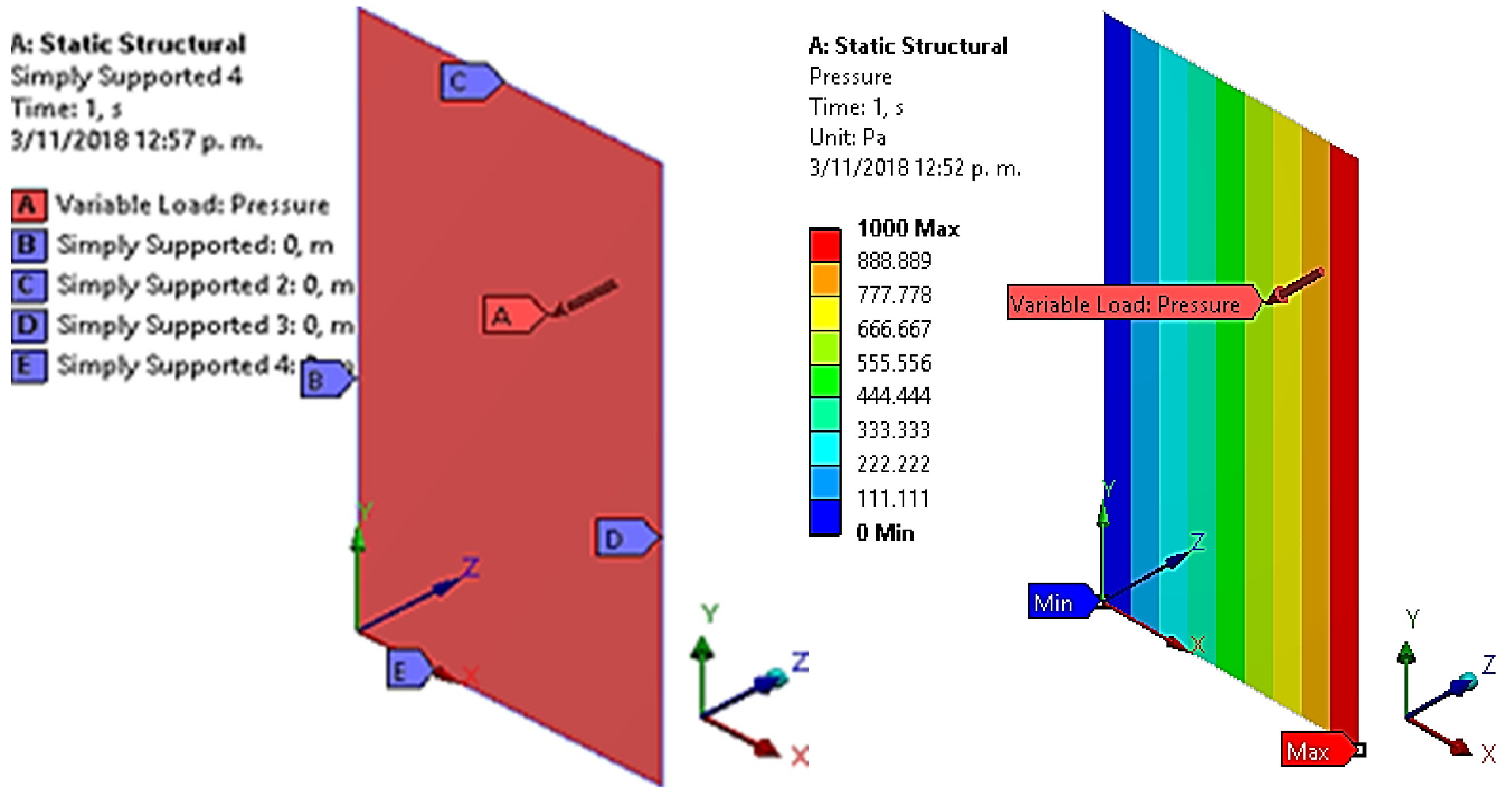
To evaluate the structural response under hydrostatic pressure, a linear pressure gradient was considered, varying from 0 to 1000 Pa along the 4 m edge. This condition is representative of structures subjected to fluid pressure, such as liquid containment plates or vessel walls.

The deflection at the center of the plate was calculated using the Fourier series expansion, considering the load coefficients and the individual contributions of each term. The analyzed plate for the hydrostatic pressure case has a length of 8 m, a width of 4 m, and a thickness of 0.02 m. The material is a heat-treated SAE 4340 steel with an elasticity module of 200 GPa and a Poisson coefficient of 0.3. Using Equations (11) and (14), the coefficients of the Fourier series (Fm,n; Cm,n) and the deflection at the center of the plate are calculated respectively (Wcenter) using the first three terms of the series. The results are shown in

Table 2. Theoretical deflection at the center points of the rectangular flat plate under hydrostatic pressure.

Term	m	n	Pm,n	Wm,n	Plate Deflection
1	1	1	8.1057 × 102	8.8618 × 10−3	8.8618 × 10−3
2	1	3	6.7547 × 10	1.3486 × 10−5	−1.3486 × 10−5
	3	1	6.7547 × 10	1.0924 × 10−4	−1.0924 × 10−4
3	1	5	4.0528 × 10	1.0859 × 10−6	1.0859 × 10−6
	3	3	2.2516 × 10	3.0390 × 10−6	3.0390 × 10−6
	5	1	4.0528 × 10	1.3172 × 10−5	1.3172 × 10−5
∑W = 8.7564 × 10−3 m

.

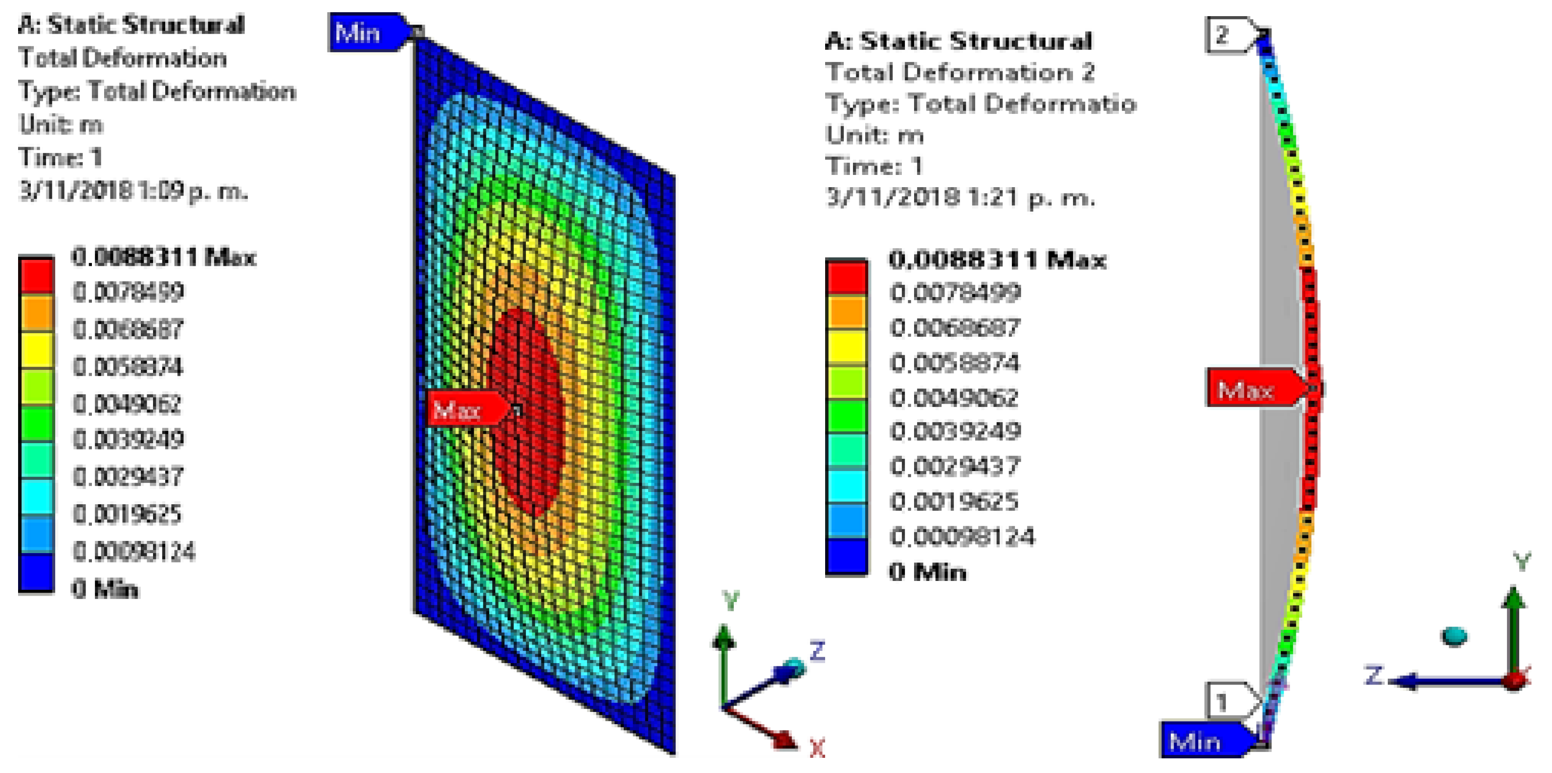
The maximum deflection at the center of the plate subjected to hydrostatic pressure was 0.0087564 m, indicating that the deformation magnitude is approximately 50% lower than that obtained under a uniformly distributed load.

The analysis was performed using a three-term approximation in the Fourier series, introducing a margin of error in the maximum deflection estimation. However, previous studies indicate that using the first three terms is sufficient to achieve an accuracy of over 95% in most cases.

To validate these results, numerical simulations will be conducted in ANSYS (Academic Version 2023) using the Finite Element Method (FEM), allowing for a comparison of the convergence between theoretical and computational values. This process is crucial for determining the optimal mesh and assessing the relative error between both methodologies.

4. Mesh Convergence

To evaluate the accuracy of the results obtained in the simulation of the maximum deflection experienced by the flat plate subjected to a triangular load, a mesh convergence study was conducted in ANSYS. Ten different mesh configurations with varying refinement levels were analyzed while keeping the material properties and boundary conditions constant. The results showed that the maximum total deformation varied from 0.0185 m in the coarsest mesh (2000 elements) to 0.016821 m in the mesh with 120,000 elements. As the number of elements increased, the maximum deformation progressively decreased, reaching values of 0.0178 m with 5000 elements, 0.0173 m with 10,000 elements, and 0.0170 m with 20,000 elements. For finer mesh configurations, the deformation continued to stabilize at 0.0169 m (40,000 elements), 0.01685 m (60,000 elements), and 0.01683 m (80,000 elements). Beyond 120,000 elements, the deformation remained constant, with values of 0.016820 m (200,000 elements) and 0.016819 m (320,000 elements). The relative difference between the mesh with 120,000 elements and the finer meshes was less than 1%, confirming the model’s convergence. As a result, the mesh with 120,000 elements was selected, as it provides an optimal balance between accuracy and computational efficiency. These results are presented in

Table 3. Maximum Deformation Accuracy as a Function of Element Count.

Number of Elements	Maximum Deformation (m)
2000	0.01850
5000	0.01780
10,000	0.01730
20,000	0.01700
40,000	0.01690
60,000	0.01685
80,000	0.01683
120,000	0.016821
200,000	0.016820
320,000	0.016819

and Figure 1.

To evaluate the accuracy of the results obtained in the simulation of the maximum deflection experienced by the flat plate subjected to a triangular load, a mesh convergence study was conducted in ANSYS. Ten different mesh configurations of varying refinement levels were analyzed while keeping the material properties and boundary conditions constant.

The results showed that the maximum total deformation varied from 0.00950 m in the coarsest mesh (2000 elements) to 0.0088300 m in the mesh with 150,000 elements. As the number of elements increased, the maximum deformation progressively decreased, reaching values of 0.00920 m with 5000 elements, 0.00900 m with 10,000 elements, and 0.00890 m with 20,000 elements. For finer mesh configurations, the deformation continued to stabilize at 0.00887 m (40,000 elements), 0.00885 m (60,000 elements), and 0.00884 m (80,000 elements). Beyond 100,000 elements, the deformation remained constant, with values of 0.00883111 m (100,000 elements), 0.0088305 m (120,000 elements), and 0.0088300 m (150,000 elements). The relative difference between the mesh with 100,000 elements and the finer meshes was less than 1%, confirming the model’s convergence. As a result, a mesh of 100,000 elements was selected, as it provides an optimal balance between accuracy and computational efficiency. These results are presented in

Table 4. Flat plate deflection mesh convergence.

Number of Elements	Maximum Deformation (m)
2000	0.00950
5000	0.00920
10,000	0.00900
20,000	0.00890
40,000	0.00887
60,000	0.00885
80,000	0.00884
100,000	0.00883111
120,000	0.0088305
150,000	0.0088300

and Figure 2.

5. Results

5.1. Finite Element Modeling and Simulation

Flat rectangular plates that are simply supported under different load conditions (uniformly distributed, triangular, and point) were analyzed using ANSYS Workbench17 software based on numerical finite element analysis techniques. The following are the steps for modeling and simulating the plate’s deflection under hydrostatic pressure, which are the same as the other two load conditions.

5.2. Definition of the Properties of the Model Material

Using the ANSYS Workbench17 program, the structural static analysis module (static structural) is enabled. In the cell corresponding to the engineering data (engineering data), a linear isotropic elastic material is selected and specified as a structural steel defined as SAE 4340 with an elasticity module = 200 GPa, a Poisson coefficient = 0.3, density 7850 Kg/m³, creep force = 250 GPa, and ultimate stress = 460 GPa.

5.3. Creation of Model Geometry

The geometric modeling process was carried out using the Design Modeler module in ANSYS. Initially, a two-dimensional rectangular sketch measuring 8 m in length and 4 m in width was created on the XY plane using the Sketching interface, employing the Draw tool for precise dimensional input. This sketch was then extruded along the Z-axis to a thickness of 0.02 m, generating a three-dimensional solid representation of a flat rectangular plate. This configuration corresponds to the geometry shown in Figure 3, which illustrates the discretized model with the associated coordinate system. The structured meshing visible in the figure confirms the defined surface topology and orientation, which is essential for subsequent finite element analysis.

5.4. Discretizing the Finite Element Serial Model

In the Mechanical module, the Mesh tool generates a mesh that has 800 Quad 4, 861 node type elements, an average aspect ratio of 1, and a mesh quality of 0.99 on average. These parameters indicate that it is an optimal mesh to perform the simulation and validation of the mathematical model. The mesh is shown in the figure. The Quad 4 element used in meshing is suitable for the analysis of thin to moderately thick laminar structures, consisting of four two-dimensional (2D) nodes with six degrees of freedom, translation, and rotation on three axes (X, Y, Z).

5.5. Boundary and Load Conditions

For the finite element analysis, a linearly varying hydrostatic pressure was applied, ranging from 0 to 1000 Pa along the shorter edge of the plate and distributed across its entire surface. This load simulates a realistic pressure condition exerted by a fluid in contact with the plate, and it was implemented using the Variable Load: Pressure feature in the ANSYS Workbench 17 environment.

Regarding boundary conditions, the plate was modeled as simply supported along all four edges. This configuration involves specific constraints on the degrees of freedom, as follows:

• Vertical translation (UZ = 0) was restricted for all edge nodes, thereby preventing displacement perpendicular to the mid-surface of the plate.
• Rotational degrees of freedom (θx, θy) were left unconstrained, allowing free edge rotation without generating fixed-end moments.
• In-plane translations (UX and UY) were permitted unless otherwise specified in the model (e.g., constraints at corner nodes to prevent rigid body motion).

This representation of simple support enables the plate to bend freely under the applied load without transmitting moments through the supports, aligning with the assumptions of classical thin plate theory under bending. Such boundary conditions are common in structural elements like slabs, bridge decks, and roofing systems, where supports function solely as vertical reactions, with no rotational restraint or moment transfer.

Both the applied load and the implemented boundary conditions are illustrated in Figure 4, which shows the distribution of pressure across the plate surface and the application of supports along each edge using the Supports tool in the Static Structural module of ANSYS Workbench 17.

In the FEM simulation, these conditions were imposed exclusively on the boundary nodes to ensure a mechanically accurate and numerically stable model. The validity of this implementation is confirmed by the low error percentages observed in the comparison between the analytical and computational results.

5.6. Problem Solution

The ANSYS Workbench17 solution folder enables us to obtain the deflection suffered by the plate, and directional deformation is activated along the Z-axis. Figure 5 shows the simulations of the deformation results obtained for the plate under hydrostatic pressure, identifying the deflection variation on the plate’s surface and its maximum and minimum points. Figure 6 shows the same results for the plate under uniform pressure.

The computational model is validated by calculating the error percentage between nine analytic (Fourier Series) and computational (ANSYS Workbench17) deflection data points taken each meter along the longest edge of the plate. Obtained results are shown in

Table 5. Percentage error of deformation in flat plate center (B = 2 M) of flat plate under hydrostatic pressure.

Deflection
a [m]	Fourier Series	FEA	Error	Mean Error
0	0	0	0	1.23%
1	3.89 × 10−3	3.99 × 10−3	2.51%
2	6.72 × 10−3	6.80 × 10−3	1.19%
3	8.23 × 10−3	8.34 × 10−3	1.43%
4	8.75 × 10−3	8.83 × 10−3	0.85%
5	8.23 × 10−3	8.34 × 10−3	1.43%
6	6.72 × 10−3	6.80 × 10−3	1.19%
7	3.89 × 10−3	3.99 × 10−3	2.51%
8	0	3.16 × 10−18	0

and

Table 6. Percentage error of deformation in flat center of flat plate (B = 2 M) under uniform pressure.

Deflection
a [m]	Fourier Series	FEA	Error	Mean Error
0	0	0	0	0.15%
1	7.62 × 10−3	7.60 × 10−3	0.24%
2	1.29 × 10−2	1.29 × 10−2	0.21%
3	1.59 × 10−2	1.59 × 10−2	0.09%
4	1.68 × 10−2	1.68 × 10−2	0.34%
5	1.59 × 10−2	1.59 × 10−2	0.09%
6	1.29 × 10−2	1.29 × 10−2	0.21%
7	7.62 × 10−3	7.60 × 10−3	0.24%
8	0	2.89 × 10−18	0

. The percentage difference in average is 0.15% and 1.23% for uniform and hydrostatic pressures, respectively.

6. Conclusions

The computational framework developed in this study demonstrates high fidelity in predicting the deflection behavior of isotropic flat plates subjected to diverse loading regimes. Its generalizability extends beyond the baseline boundary conditions assessed, rendering it suitable for a broad spectrum of structural configurations and loading environments. Through parameter tuning and model reconfiguration, the methodology can be adapted to accommodate complex load profiles, anisotropic or heterogeneous material properties, and non-conventional plate geometries. This methodological flexibility positions the model as an asset for advanced structural mechanics and computational engineering applications.

The analytical determination of plate deflections, particularly under realistic loading and boundary conditions, is mathematically intensive and often limited to idealized scenarios. Such methods necessitate closed-form solutions derived from partial differential equations, which become intractable under complex geometrical or loading configurations. In contrast, the Finite Element Method (FEM) offers superior adaptability, enabling the resolution of nonlinearities, irregular boundary conditions, and spatially varying loads. For load cases involving stochastic or non-uniform pressure fields, analytical approaches may lack feasibility. In such instances, a robust computational model obviates the reliance on costly and time-consuming experimental procedures while maintaining high predictive accuracy.

In the context of FEM implementation within ANSYS, solution accuracy is critically dependent on mesh discretization strategies, element formulation, and topological quality. Fine meshes with optimized aspect ratios and well-conditioned elements are essential for capturing the structural response with minimal numerical dispersion. The mesh resolution directly influences the convergence of the solution and the accuracy of stress and displacement fields. Conversely, coarse or poorly shaped elements may induce singularities, spurious stress concentrations, or convergence instabilities, thereby degrading the credibility of the simulation. As such, the implementation of adaptive mesh refinement protocols and rigorous convergence analysis is imperative for achieving numerically stable and physically representative solutions in structural plate analyses.