Abstract
This work establishes a simple algorithm to recover an information vector from a predefined database available every time. It is considered that the information analyzed may be incomplete, damaged, or corrupted. This algorithm is inspired by Hopfield Neural Networks (HNN), which allows the recursive reconstruction of an information vector through an energy-minimizing optimal process, but this paper presents a procedure that generates results in a single iteration. Images have been chosen for the information recovery application to build the vector information. In addition, a filter is added to the algorithm to focus on the most important information when reconstructing data, allowing it to work with damaged or incomplete vectors, even without losing the ability to be a non-iterative process. A brief theoretical introduction and a numerical validation for recovery information are shown with an example of a database containing 40 images.
1. Introduction
Hopfield neural networks (HNN) are a tool with a simple recurrent structure and with an efficient associative memory in which a search and recognition of patterns are performed [1], where the search for patterns is obtained by minimizing the energy, which can be obtained as long as there is a change in the input [2]. In addition, these networks can be trained in continuous time in a deterministic way representing Amari’s gradient [3], and it is known that it can solve combinatorial optimization problems. However, it is only sure that convergence to a local minimum is obtained if the problem can be written in terms of an energy function [4]. Applications of this type of data-driven neural networks are found in various sectors, such as medicine [5], in robotics solving the traveling salesman problem (TSP) [6], for mathematical modeling based on pattern recognition and system knowledge [7]. Reference [8] shows an approach to performing image segmentation using Hopfield neural networks applying constraints on the edges of the figure, where a probability-based pixel difference criterion is performed, and the neural network automatically adapts this probability to find optimal or suboptimal segmentation results. For the Hopfield neural network, in the computational sense, ideas for solving weighted constraint problems continue to appear [9]. Some of the applications for HNN also have comparisons with other types of tools, such as artificial immune systems (AIS), from which ideas are derived to solve computational problems that generate an optimal result with constraints such as obtaining Boolean satisfiability using the MAX-kSAT problem [10,11]. Also, it can be possible to determine the stability of HNN networks and perform the segmentation of objects in images [12]. However, when the image has multi-modal information, it is more complicated to get the results, so they apply a neural network to measure the threshold levels in the objects in gray scales in an adaptive way [13].
For the training of Hopfield neural networks, alternatives have been developed for the minimization of the energy or generate structure additions to have improvements, such as the change of the search for an optimum using the Moore-Penrose pseudo inverse [14], or even appearing alternative neural networks such as oscillatory neural networks (ONN) that can work as self-associative memory networks that have comparative with Hopfield neural networks due to their operation [15]. In the case of an application for images, it is also possible to change the function to minimize Hopfield neural networks to obtain the limits of the images while minimizing this function [16]. Knowing which neurons have much or little noise, it is possible to reinforce the neurons with little noise to improve the tolerance to this [17]. Also, ways to train neural networks can be found in [18], where the training idea is presented for feed-forward networks based on energy minimization with two steps: unsupervised learning in the first step to obtain the weights that relate the inputs with the neurons and network parameters, and the second step to perform the backpropagation of the internal and external energy to the network structure. However, all this is iterative to achieve the goal.
With the evolution of the Hopfield neural networks, it has been attempted to eliminate the information that is not part of the data, such as noise in the transmission of messages [19]. They are also being used to recover a set of correct data from a database when having corrupted information, with an approximate or compressed associative memory matrix [20]. In addition, implementing these neural networks using a Field Programmable Gate Array (FPGA) has been achieved without losing the advantages that the neural network provides, such as eliminating noise in the information [21]. There are even applications of this type of neural network using memristors, with good robustness against memristive variations and noises in the input, for restoring images [22].
In this work, we seek to implement algorithms for data recovery, specifically images, using non-iterative processes and compare it with information retrieval using the HNN network: (1) propose the theoretical background for the implementation of a non-iterative process for information recovery where a metric is established between actual data and data in an image database to determine similarity; (2) establish a methodology that achieves information recovery from a database using an unsupervised HNN; (3) create an algorithm that generates information recovery in a single iteration; and (4) present an extension of the algorithm to weighted information vectors.
The structure of this document is as follows: Section 2 shows a mathematical background and basic vector operations as well as the mathematical ideas of Hopfield neural networks. Section 3 contains the ideas for applying the HNN and the author’s algorithms presented for this work. Section 4 contains an image data-driven example for information retrieval using the algorithms proposed by the authors. Section 5 and Section 6 present the discussion and conclusions for this work, respectively.
2. Materials and Methods
2.1. Theoretical Background
In the computational field, vectors can be called database elements because they represent a data set as an array. These vectors have the following definitions and properties:
Definition 1.
Consider a non-empty finite set of column vectors , with and same dimension, number of positive data as input, and form of non-proportional even vectors can form a database for recovery information.
This must not represent a basis of a vector subspace; moreover, is not a vector space. It is only a set in which constant information can be stored. In addition, for this case, with which it is possible to construct the database matrix as follows:
Considering the inner product of two vectors as and to each vector can be applied the Euclidean norm with the form . The Euclidean norm represents an unbounded function, so applying information theory would be better if a bounded norm were used to induce a finite metric to compare the similarity of two vectors.
Lemma 1.
Consider and with , then
Proof.
Consider the math operations:
□
Proposition 1.
For two vectors ( is not a vector subspace) the function given by
This represents an induced bounded metric.
Proof.
By construction, the following is known , adding the inner product properties it follows that and due to the Cauchy–Schwarz inequality if implies , then note that
where is the Euclidean metric. Consider that the function with and with satisfies , if clearly and by Lemma 1 then by properties of metric is:
and applying yields:
where is a non-zero vector. Finally, this metric is bounded by the Cauchy–Schwarz inequality. □
This metric is suitable for data recovery applications to quantify the similarity of two information vectors. For choosing q, it is considered that a significant value better detects subtle differences in data vectors but increases the computational error metric due to computational limitations.
2.2. Hopfield Neural Network as Associative Memory
The main idea of unsupervised neural network algorithms is to train or test with the correlation between vectors or matrices of information to minimize an energy function. For a database with matrix X and a unit column vector , in which the information may be missing or corrupted, is required to recover the correct information column vector of the database starting with the value in . To solve this problem, the authors in [23] found an interesting energy functional as follows:
where M is the most significant Euclidean norm of all stored patterns and:
with and . It is necessary to find as a value that minimizes Equation (8). The functional has concave and convex terms in which the Concave-Convex Procedure (CCCP, see [24]) is applied:
where is the iteration number. Substituting yields:
taking the gradients:
where the Equation (12) generates information for each iteration in the following form:
with the calculation of the softmax function as follows.
for every .
For procedure in Equation (12) choice large enough (see [24]), this is important to obtain a fast convergence.
The recovery of the data by the HNN network can be obtained by the Algorithm 1, which follows the idea presented in [23]. This algorithm obtains energy minimization (see Theorem 3 in [24]). For this, construct the matrix X with the vector for which we calculate recursively r times the value of , and at the end, we select the value of that minimizes the Equation (8).
| Algorithm 1 Information recovery with HNN-based method. |
|
2.3. Interpretation
The procedure in Equation (12) represents a correlation vector with a maximum approximation having a softmax function produced by the inner products with elements of and , i.e.:
Then, the softmax function returns a normalized discrete distribution of the inner products, and results in a linear combination of elements of with the closest component to . In every iteration, this distribution tends to a specific element or oscillates around a set of vectors that minimize Equation (8) (see [24]).
Proposition 2.
The Algorithm 1 minimizes the metric for every .
Proof.
An important property of the softmax function is
for implies , then, in every iteration, k obtains a linear convex combination. Consider the identity of the following equation:
with where and consider by the properties, the index r is choose like the maximum in the set for a fixed , by properties of a metric and Cauchy–Schwarz inequality implies minimizing the set for every k iteration then the distribution converges or oscillates and converges or oscillates around minimum points of (see [24]). □
A necessary consequence of this procedure is that the convergence does not guarantee a closed solution of the minimization problem because it is not necessarily for then is not necessarily zero.
3. Proposed Procedure
Inspired by the interpretation of the Algorithm 1, it is possible to generate a method containing a simple procedure for information recovery. The authors propose algorithms that generate information recovery in only one iteration as follows:
where .
Equation (18) represents the non-iterative methodology of information recovery by simultaneously comparing the actual information with the whole database. This methodology may have fewer computational operations compared to the Algorithm 1.
Proposition 3.
For a database and a normalized column vector the method in Equation (18) minimizes the metric for every .
The construction of the procedure using the Algorithm 2 allows obtaining proof of this proposition and does not require further considerations. It is essential to mention that this minimum is not necessarily unique.
The procedure compares the actual information with the information contained in the database using a metric as stated in the Equation (4), and at the end, r is selected, which includes the information from the database that has the slightest difference between the data. These steps can follow as:
| Algorithm 2 Recovery Procedure (RP). |
|
3.1. Capacity of Reconstruction
Definition 2.
The capacity of reconstruction of is defined as:
A brief interpretation is that consider the worst case of confusion to select the correct index r in Algorithm 1 or Algorithm 2 for some . That is where is the correct vector information and is noise or data corruption. If is such that is closest to another information vector , then the algorithms return the incorrect recovery data vector.
If the capacity of reconstruction is small, then there exists a the possibility that some corrupted information vectors cannot be reconstructed adequately.
3.2. Extension to Weighted Information Recovery Procedure
To improve the idea presented in the previous algorithms, the authors propose adding a filter with multiplicative properties applied to specific information sections to focus on certain areas of interest, e.g., parts of the information that have less damage or corruption.
For the application of the filter in the information, we have the following vector properties:
Definition 3.
For the Hadamard product is defined as:
where U and V are vectors with information of the following form:
The operation in Equation (20) represents the classic element-by-element product in vectors.
Definition 4.
The operation filter information from vector where , indicating that it is weighted filter for U. In extension to a database, defines as a weighted filtered database.
These filters highlight the relevant information in the vector to be retrieved and ignore the terms that are not of great interest. Radial Gaussian functions and Heaviside functions, among others, can also give these filters. For example, Figure 1 presents on the left an image that has gone through a process to convert it into vector information; in the center of the figure is the figure when a Gaussian filter is applied, and on the right is the same image with the application of a Heaviside filter.
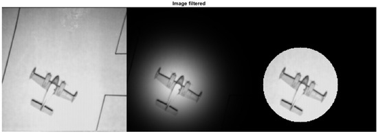
Figure 1.
Image with weighted filters.
The extension of the Algorithm 2 to which the passing of the information through a filter is added can be performed with the following steps:
The Algorithm 3 has the information as an array of vectors, and by applying the filter as established in Definition 4 generates vectors with specific details of the actual data to compare with the available database, step 2 calculate the difference between the actual data and the data in the database using the metric proposed in the Equation (4) and finally, selected r where the slightest between data difference is yielded in step 3.
| Algorithm 3 Weighted Recovery Procedure (WRP). |
|
4. Results
Numerical Example
This section will generate information recovery by constructing vectors from image data. The algorithms proposed earlier have been applied to image recovery since the database includes images. For this purpose, consider a database that contains 40 grayscale images, each with a size of pixels. The image database is available in [25] and is illustrated in Figure 2.
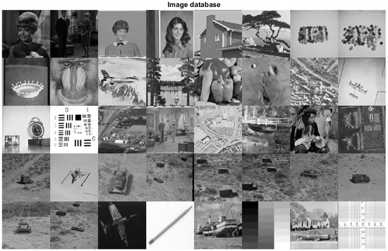
Figure 2.
Gray-scale image database.
In this database, each image is a matrix where a reshape is applied to convert the information into vectors that are found in with m = 40,000.
Image recovery is then applied using the algorithm presented for HNN. At the top of the Figure 3 are the images containing corrupted or damaged information, while at the bottom is the recovery of the image containing the filter using Algorithm 2. Note that the reconstruction is efficient except for the last image, where an image that does not belong to the database was intentionally introduced. Then, the algorithm takes the information that most closely represents the image from the information that does belong to the database.
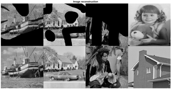
Figure 3.
Recovery information from corrupted image.
With the results obtained in Figure 3 generate the Table 1 that compares the algorithms proposed in this work, where the metric with and is used. Two different numbers of iterations have been considered for the Algorithm 1, but there is only one iteration for applying the Algorithm 2. Table 1 correlates the corrupted image data and the image data in the database. In the first row, where this correlation shows results close to zero, it marks a closeness between the images. However, in this way, it cannot determine who has more accuracy because they all have high correlations. Because of this, the norm in the Equation (4) is used to know who has more closeness between the data of the actual image and the data in the database, obtaining in the second row the closeness between the pictures when one iteration is performed in the algorithm for HNN. Also, the third row shows the closeness of results when there are more iterations, so the results are closer to zero. Finally, in the last row, the closeness between images is determined using Algorithm 2, and the correct image is obtained in a single iteration because the difference is zero.

Table 1.
Brief statistics comparing the algorithms.
The metric compares between the correct and recovered images, except for image 4, where the comparison is with the closest image in the database. Note that for the first three images, iterating with the Algorithm 1 converges to zero, but the proposed Algorithm 2 achieves convergence in a single iteration where it reaches the selection of the correct image considering the database. For image four, the algorithms attempt to recover the house in the database, not the girl and the teddy bear, so the final metric is non-zero in the proposed algorithm. This property reveals that the algorithm can correctly recover the information if there is information in the database.
In example 2, we consider a given corrupted image with different Gaussian noise levels, as shown in the first row of Figure 4, where it has randomly uniform degradation contamination set to zero oscillating with , , , , and of corrupted information from left to right, respectively. These percentages mark the probability that a pixel is corrupted or not. Applying Algorithm 2 calculates the metric between corrupted information and the information in the database, where the result is the nearest image to the actual data. The results using Algorithm 2 are shown in the second row of Figure 4. A Heaviside filter is applied for the corrupted image, as shown in Figure 5, together with Algorithm 3 to work with the essential information of each image, generating the third-row results in Figure 4.
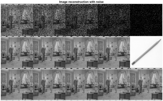
Figure 4.
Image reconstruction for different noise levels.
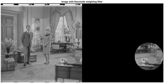
Figure 5.
Heaviside filter to improve the accuracy.
It is clarified that the filter should be applied where the information is most relevant according to the context of the importance of the data. Table 2 shows a comparison of the recovery of the images by the algorithms proposed by the authors in this work, where the results of recovery of the information are observed, although it has different levels of damage in the original data, without forgetting that this is achieved by only one iteration in its operation and reviewing the metric dictates that the difference tends to zero. The first row of the Table 2 contains information on the probability of damage contained in the pixels in each image. In contrast, rows two and three show the difference between the real data and the information in the database, so it can be determined that the trend toward zero value means the actual information is recovered. However, in the last column, it can be observed that when a filter is applied while the algorithm is being performed, it improves the image recovery capacity, generating the correct image, while when the filter has not applied, the algorithm gives the closest information as it can be observed in the Figure 4.
Table 2.
Comparison of the Algorithms 2 and 3.
5. Discussion
The application of the algorithms for the information recovery procedure by a database proposed in this work manages to recover the data without the need to perform iterative computational operations. Applying the Equation (18), fewer computational operations have been performed compared with the procedure using HNN, where, although the recovery of the data can be obtained, several steps (iterations) are required to have convergence. In applying the non-iterative methodology, it is possible to visualize that good information recovery is achieved, even if it is damaged or corrupted, so the application of the algorithm is still good, even if it is only one or a few steps to obtain that information. It is also worth mentioning that adding a filter to focus on a section of the data to be recovered does not generate more computational operations. It maintains the advantage of data recovery with a high correlation, so the procedure is still achieved in a single iteration.
Although the results obtained by the algorithms presented in this work are reasonable, there is a significant dependence on the database used to perform the information recovery, so it is possible to think of future work in applying generative information tools to reconstruct the corrupted data. Also, when a large part of the information is lost, it is possible not to obtain a good recovery of these by the algorithms, so it is possible to add tools that select the essential information of the data, such as the principal component analysis (PCA).
6. Conclusions
Hopfield’s neural networks as associative memories can recover information contained in a database, and this idea serves as the primary basis for the formation of the algorithms developed in this work. It is important to mention that the database can contain information of any type, such as audio or video or, as illustrated in this work, image information. With the analysis of the results obtained in the examples presented in Section 4, it is observed that it was possible to recover information from a database containing images in a single iteration, even when it contains corrupted information. Applying the Algorithm 3 shows that the procedure can focus on the critical information contained in the image by applying a filter, but this still gets results in a single iteration. Since the procedures proposed in this work are performed in a single iteration, fewer computational operations are present when executed, which may present an advantage against iterative algorithms. On the other hand, applying the metric presented in the Equation (4) can demonstrate whether there is a good convergence and shows more detail on the difference between the actual data and the data obtained in the information recovery.
Author Contributions
Formal analysis, C.U.S., J.M. and C.M.M.; Methodology, C.U.S., J.M. and C.M.M.; Writing – original draft, C.U.S.; Writing – review & editing, J.M. and C.M.M. All authors have read and agreed to the published version of the manuscript.
Funding
The Instituto Politecnico Nacional research projects with SIP numbers 20241511, 20241721, 20250424 and 20253411 funded this work.
Informed Consent Statement
Not applicable.
Data Availability Statement
The database shown in the Figure 2 is a database available to anyone created by open images at https://storage.googleapis.com/openimages/web/download_v7.html, (accessed on 10 September 2024), for more information see reference [25].
Acknowledgments
The authors would like to thank the Instituto Politécnico Nacional for their valuable support during the development of this research, as well as the funding provided by the IPN-SIP (SIP 20241721, 20241511, 20250424, and 20253411) and the Sistema Nacional de Investigadoras e Investigadores de México. The author, Cesar U. Solis, dedicates this work to his daughter, Sandra Ekaterina.
Conflicts of Interest
The authors declare no conflicts of interest with this journal or any other journal or institution.
References
- Rojas, R. Neural Networks: A Systematic Introdution; Springer Science and Business Media: New York, NY, USA, 2013. [Google Scholar]
- Hopfield, J.J.; Tank, D.W. “Neural” computation of decisions in optimization problems. Biol. Cybern. 1985, 52, 141–152. [Google Scholar] [CrossRef] [PubMed]
- Halder, A.; Caluya, K.F.; Travacca, B.; Moura, S.J. Hopfield Neural Network Flow: A Geometric Viewpoint. IEEE Trans. Neural Networks Learn. Syst. 2020, 31, 4869–4880. [Google Scholar] [CrossRef] [PubMed]
- Gil, J.; Martinez Torres, J.; González-Crespo, R. The application of artificial intelligence in project management research: A review. Int. J. Interact. Multimed. Artif. Intell. 2021, 6, 1–13. [Google Scholar] [CrossRef]
- Neshat, M.; Zadeh, A.E. Hopfield neural network and fuzzy Hopfield neural network for diagnosis of liver disorders. In Proceedings of the 2010 5th IEEE International Conference Intelligent Systems, London, UK, 7–9 July 2010. [Google Scholar] [CrossRef]
- Zhong, C.; Luo, C.; Chu, Z.; Gan, W. A continuous hopfield neural network based on dynamic step for the traveling salesman problem. In Proceedings of the 2017 International Joint Conference on Neural Networks (IJCNN), Anchorage, AK, USA, 14–19 May 2017; pp. 3318–3323. [Google Scholar] [CrossRef]
- Ma, X.; Zhong, L.; Chen, X. Application of Hopfield Neural Network Algorithm in Mathematical Modeling. In Proceedings of the 2023 IEEE 12th International Conference on Communication Systems and Network Technologies (CSNT), Bhopal, India, 8–9 April 2023; pp. 591–595. [Google Scholar] [CrossRef]
- Sang, N.; Zhang, T. Segmentation of FLIR images by Hopfield neural network with edge constraint. Pattern Recognit. 2001, 34, 811–821. [Google Scholar] [CrossRef]
- Haddouch, K.; Elmoutaoukil, K.; Ettaouil, M. Solving the Weighted Constraint Satisfaction Problems Via the Neural Network Approach. Int. J. Interact. Multimed. Artif. Intell. 2016, 4, 56–60. [Google Scholar] [CrossRef][Green Version]
- Bin Mohd Kasihmuddin, M.S.; Bin Mansor, M.A.; Sathasivam, S. Robust artificial immune system in the Hopfield network for maximum k-satisfiability. Int. J. Interact. Multimed. Artif. Intell. 2017, 4, 63–71. [Google Scholar]
- Kasihmuddin, M.S.B.M.; Mansor, M.A.B.; Sathasivam, S. Genetic algorithm for restricted maximum k-satisfiability in the Hopfield network. Int. J. Interact. Multimed. Artif. Intell. 2016, 4, 52–60. [Google Scholar]
- Faydasicok, O. A new Lyapunov functional for stability analysis of neutral-type Hopfield neural networks with multiple delays. Neural Netw. 2020, 129, 288–297. [Google Scholar] [CrossRef] [PubMed]
- Rout, S.; Srivastava, P.; Majumdar, J. Multi-modal image segmentation using a modified Hopfield neural network. Pattern Recognit. 1998, 31, 743–750. [Google Scholar] [CrossRef]
- Cursino, C.; Dias, L.A.V. Extended hopfield neural network: A complementary approach. Neural Netw. 1988, 1, 225. [Google Scholar] [CrossRef]
- Jiménez, M.; Avedillo, M.J.; Linares-Barranco, B.; Núñez, J. Learning algorithms for oscillatory neural networks as associative memory for pattern recognition. Front. Neurosci. 2023, 17, 1257611. [Google Scholar] [CrossRef] [PubMed]
- Dawei, Q.; Peng, Z.; Xuefei, Z.; Xuejing, J.; Haijun, W. Appling a Novel Cost Function to Hopfield Neural Network for Defects Boundaries Detection of Wood Image. Eurasip J. Adv. Signal Process. 2010, 2010, 427878. [Google Scholar]
- Kobayashi, M. Two-Level Complex-Valued Hopfield Neural Networks. IEEE Trans. Neural Networks Learn. Syst. 2021, 32, 2274–2278. [Google Scholar] [CrossRef] [PubMed]
- Wang, J.; Chen, J.; Zhang, K.; Sigal, L. Training feedforward neural nets in Hopfield-energy-based configuration: A two-step approach. Pattern Recognit. 2024, 145, 109954. [Google Scholar] [CrossRef]
- Gladis, D.; Thangavel, P.; Nagar, A.K. Noise removal using hysteretic Hopfield tunnelling network in message transmission systems. Int. J. Comput. Math. 2011, 88, 650–660. [Google Scholar] [CrossRef]
- Deb, T.; Ghosh, A.K.; Mukherjee, A. Singular value decomposition applied to associative memory of Hopfield neural network. Mater. Today Proc. 2018, 5, 2222–2228. [Google Scholar] [CrossRef]
- Mansour, W.; Ayoubi, R.; Ziade, H.; Velazco, R.; El Falou, W. An optimal implementation on FPGA of a hopfield neural network. Adv. Artif. Neural Syst. 2011, 2011, 189368. [Google Scholar] [CrossRef]
- Hong, Q.; Li, Y.; Wang, X. Memristive continuous Hopfield neural network circuit for image restoration. Neural Comput. Appl. 2020, 32, 8175–8185. [Google Scholar] [CrossRef]
- Krotov, D.; Hopfield, J. Large associative memory problem in neurobiology and machine learning. arXiv 2020, arXiv:2008.06996. [Google Scholar]
- Yuille, A.L.; Rangarajan, A. The Concave-Convex Procedure. Neural Comput. 2003, 15, 915–936. [Google Scholar] [CrossRef] [PubMed]
- Googleapis.com. Open Images V7- Download. 2022. Available online: https://storage.googleapis.com/openimages/web/download_v7.html (accessed on 10 September 2024).


Disclaimer/Publisher’s Note: The statements, opinions and data contained in all publications are solely those of the individual author(s) and contributor(s) and not of MDPI and/or the editor(s). MDPI and/or the editor(s) disclaim responsibility for any injury to people or property resulting from any ideas, methods, instructions or products referred to in the content. |
© 2025 by the authors. Licensee MDPI, Basel, Switzerland. This article is an open access article distributed under the terms and conditions of the Creative Commons Attribution (CC BY) license (https://creativecommons.org/licenses/by/4.0/).