1. Introduction
Currently, analog circuit has become an important pillar in military, national defense, aviation and other fields. Therefore, accurate and efficient fault diagnosis of analog circuits has become a research hotspot in the field of circuit testing [
1,
2,
3]. According to statistical data, electronic circuits are developing in the direction of high integration and high complexity, in which the fault rate of analog circuits is more than 80%, which easily leads to frequent accidents, financial losses, and even casualties [
4,
5,
6]. Hence, analog circuit fault diagnosis technology is regarded as a key technology in ensuring the normal operation of electronic equipment. Early and accurate diagnosis of analog circuit faults can help further predict the fault time of the analog circuit, calculate the residual effective performance of the circuit, reduce the fault rate of the analog circuit and improve its operational efficiency. Thus, developing an effective and fast electronic circuit diagnosis strategy has become an urgent need in the field of analog circuit fault diagnosis [
7].
Early analog circuit fault diagnosis relied on the fault dictionary model, which matches faults by pre-storing fault patterns. This approach enables fast matching and reduces computational costs in small-scale circuits or scenarios with limited fault patterns. However, as circuit complexity increases, traditional methods face challenges: they rely on a complete fault dictionary, which is costly to construct, and their accuracy declines under noise or environmental interference, limiting their applicability in complex circuit diagnosis. Li et al. [
8] proposed a novel joint peak-to-peak analysis and worm analysis threshold method to address fault detection in locally nonlinear fuzzy autonomous ground vehicle systems with disturbances by establishing a set membership estimation. Ding et al. [
9] studied the dynamic response of the Hodgkin–Huxley neuron model under periodic excitation. By using a phase return map, they converted the neuron firing signals into a 1D mapping and quantified the differences between chaotic and periodic states through symbolic dynamics, demonstrating the method’s applicability in transient signal analysis of power electronic device faults.
These studies show that with the continuous development of fault diagnosis technology, more and more innovative methods have been proposed and applied in different fields. Meanwhile, with the rapid development of the semiconductor industry, the demand for more advanced circuit fault diagnosis techniques has become increasingly urgent. To address this, data-driven knowledge-based methods were introduced to solve the inefficiency of traditional fault diagnosis. Wang et al. [
10] proposed an improved spiking neural network (ISNN) for intershaft bearing fault diagnosis. They developed an encoding method to convert raw vibration data into spike sequences and validated its accuracy and effectiveness. To quickly learn and adapt to time-series tasks, Wang et al. [
11] developed an improved echo state network (IESN) for fault diagnosis of tractor power shift systems. By simulating 30,000 sets of test data and using an enhanced dynamic time warping algorithm for data segmentation, the improved ESN was used to classify fault samples. The results show that the improved ESN outperforms traditional algorithms in both training speed and accuracy. After neural networks achieved high diagnostic accuracy, research on fault diagnosis based on machine learning methods became a popular research area [
12].
Binu et al. [
13] designed a Ride NN classifier using a rider optimization algorithm to optimize neural network (NN); Zhang et al. [
14] proposed a fault diagnosis method based on unsupervised clustering to improve support vector machine (SVM). Although machine learning has achieved high performance in fault diagnosis, two major drawbacks still limit its development: (1) the hyperparameters in classification models are mostly set empirically, making the diagnosis results highly influenced by human factors; (2) shallow learning models are not suitable for large-scale data environments and tend to overlook potential features. In recent years, deep learning methods have been widely applied in fault diagnosis [
15,
16,
17] due to their powerful data feature extraction capabilities and excellent ability [
18] to describe nonlinear fault dynamics [
19].
Among deep learning methods, deep belief networks (DBNs) have proven effective in multi-layer unsupervised learning and supervised fine-tuning. By extracting key features of data through multiple nonlinear transformations, DBNs can be applied to fault diagnosis [
20,
21,
22]. Chen et al. [
23] proposed a DBN-based fault diagnosis method for analog circuits, which can adaptively extract features from time-series signals and automatically classify faults. However, DBNs have limitations in handling complex fault patterns and optimal classification within the same category. The lack of refined classification may affect the overall model performance, particularly in dynamic and diverse fault scenarios. To address this issue, Su et al. [
24] used a DBN to extract deep features from the output signal of analog circuits and optimized the support vector machine (SVM) using gray wolf optimization (GWO), resulting in the GWO-SVM model for diagnostic classification. Experimental results show that this method significantly improves diagnostic accuracy and shortens diagnosis time. However, DBNs still struggle with the 2D image structure and perform poorly when handling large high-dimensional datasets. As a result, researchers have begun to explore alternative deep-learning architectures. For example, Lee et al. [
25] proposed a convolutional deep belief network (CDBN), which effectively addresses the challenges of high-dimensional images and can scale these images effectively. However, when large datasets are involved, the CDBN model tends to overfit. To solve this issue, Goodfellow et al. [
26] introduced generative adversarial network (GAN), which can alleviate the overfitting problem and reduce the reliance on large datasets [
27]. He et al. [
28] proposed to use the cross wavelet transform (XWT) to capture features, regularize and construct three-channel feature image data, build a model with convolutional neural network (CNN), and extend GAN into a supervised classifier. Experiments show that GAN can alleviate over-fitting and reveal the nonlinear relationship between fault source and fault feature, and has a good application prospect in analog circuit fault diagnosis. However, GAN requires a longer training time, and the quality of the generated samples is also difficult to control. Therefore, it still faces challenges in stability and optimization, especially in real-world environments with noisy or incomplete data. Despite the potential of DBN and GAN, they still fall short of fully addressing the complexity and accuracy requirements of analog circuit diagnosis.
To fully leverage the temporal correlation features of analog circuit signals, enhance the model’s ability to mine data, and improve fault classification accuracy, CNN has gradually become a key focus in the research of analog circuit fault diagnosis due to their powerful feature extraction capabilities. Kim et al. [
29] found that CNN has enough acceptance ability in the frequency domain and time domain, but it has poor generalization ability in the time domain and high acceptance ability in the complex frequency domain, and thus it is concluded that the choice of working domain is related to the network model. Du et al. [
30] suggested to use CNN to carry out analog circuit fault diagnosis. The experimental results of Sallen-Key filter circuit show that CNN can effectively simplify the fault diagnosis process and improve the fault diagnosis rate. Zhang et al. [
31] proposed a new analog circuit soft fault diagnosis method, which combines the backward difference strategy with CNN and the global average pooling (GAP), the former performs data processing, while the latter carries out fault diagnosis and classification. Experimental results show that this method has good applicability in the field of analog circuit fault diagnosis. However, the importance of the information in each channel is different in practice, while the traditional CNN defaults to the equal importance of each channel’s information and lacks the screening of important features. Therefore, squeezed excitation networks (SENet) and selective kernel networks (SKNet) are proposed to optimize CNNs in terms of dimensionality and convolutional kernels [
32,
33]. The theory suggests that while networks with deeper structures may obtain higher performance, they are also more prone to gradient disappearance or explosion, leading to slow convergence and over-fitting problems [
34]. Therefore, He et al. [
35] proposed a deep residual network (ResNet) structure, which addresses the problem of performance degradation due to increasing network depth, resulting in a higher performance of the whole network. Considering the long training time and low unsupervised learning accuracy of residual networks, from the perspective of improving the training speed and accuracy, Zhou et al. [
36] improved the structure of ResNet by combining SE-Net and multi-level depth feature fusion. Tong et al. [
37] embedded a multi-scale deep separable expression recognition network based on convolutional block attention module (CBAM) in the residual network to improve the weight of important features in the network, eliminate irrelevant redundant features and enhance the robustness of the network. Tang et al. [
38] utilized multi-input convolution to combine time domain and frequency domain to accurately extract features, and the experimental results show that the proposed model can improve the recognition rate and convergence performance of the traditional convolution model, and has good robustness and generalization ability.
Most of the above literature only studies the problem of analog circuit fault from the perspective of time domain or frequency domain, while deep learning has some problems in fault diagnosis, such as complex models and difficulty in extracting essential features. In order to comprehensively capture the time domain feature information and frequency domain feature information, the multiple-convolutional neural network (MI-CNN) model is considered as the basic framework for the extraction of the special whole. Meanwhile, in order to improve the performance degradation of deep learning due to the deepening of network structure, the ECA module is used to optimize the model. Therefore, a model based on ECA-MI-CNN is constructed in this paper. Based on single-input CNN, the proposed model uses MI-CNN to realize information fusion, and ECA module is added in the feature extraction process to reduce the computation on the premise of ensuring network performance. Taking the fault diagnosis of Butter-worth low-pass filter and two-stage quad op-amp dual second-order low-pass filter as examples, the comprehensive performance of the ECA-MI-CNN model is verified by several comparison experiments.
2. ECA-MI-CNN
2.1. Traditional CNN and BN Layer
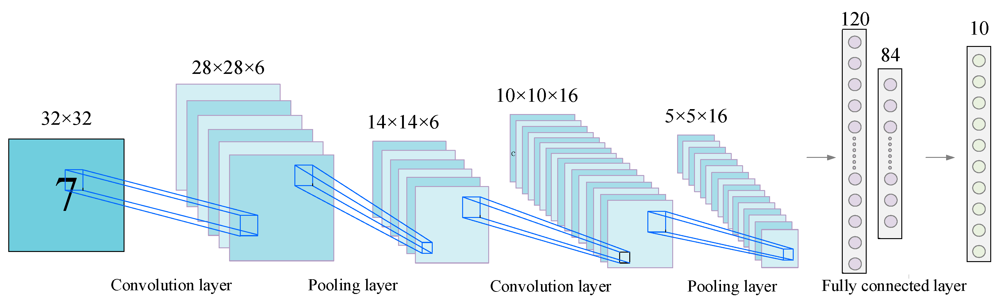
CNNs are outstanding in the field of image data with the advantage of convolutional operations, and the typical structure is shown in
Figure 1.
The convolution layer is a convolutional operation to extract features from the information in the perceptual field by means of a designed convolutional kernel, as shown in (1):
where
is the number of layers at the time of model building,
is the activation function chosen,
is the
k-th feature mapping of the
l-1th layer,
is the individual convolution kernel, and
is the bias.
CNN can extract features efficiently. In addition, the local connectivity and shared weights used by CNN reduce the complexity of deep networks, and on the other hand reduce the risk of overfitting. However, deep neural networks suffer from difficulties in training and slow convergence as the network depth deepens. The addition of a batch normalization (BN) layer after the convolutional layer can effectively improve the problem.
The conduction process of the BN layer is as follows:
- (1)
Calculation of sample average.
where
m is the number of samples and
x is the sample.
- (2)
Calculation of sample variance.
- (3)
Standardization of sample data.
where
is a random value that ensures the denominator is not 0.
- (4)
Perform translation and scaling processing.
where
and
are learning parameters.
2.2. MI-CNN
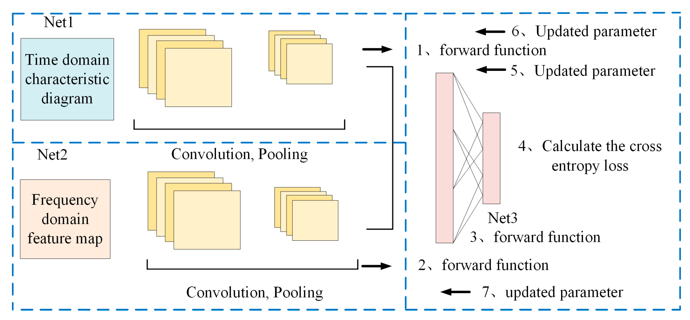
The advantage of the MI-CNN feature fusion framework is that it matches different convolutional and pooling strategies for different features, fully utilizing the feature extraction capability of the convolutional neural network, and finally fusing and feeding the higher-order features to the Softmax layer to select and non-linearly fit the extracted higher-order features, greatly improving the classification performance of the network. The process of the MI-CNN structure is shown in
Figure 2:
- (1)
Input Stage: The input images are fed into two independent subnetworks, Net1 and Net2, for feature extraction.
- (2)
Feature Extraction: Net1 and Net2 employ different convolution and pooling strategies to extract features at various levels and forward the information.
- (3)
Feature Fusion: The extracted features from Net1 and Net2 are fused in the fully connected layer of Net3 to effectively integrate the information from different networks.
- (4)
Classification Calculation: The fused high-order features are passed to the Softmax layer for classification, and the cross-entropy loss is computed.
- (5)
Backpropagation: The computed loss is propagated backward to optimize the weights and biases in Net3.
- (6)
Parameter Update: The parameters in Net1 and Net2 are updated to enhance feature extraction capability and improve the overall classification performance of the network. Net1 and Net2 are, respectively, used for operations such as convolution and information forwarding.
2.3. ECA Module
In recent years, studies have demonstrated that channel attention has significant potential to enhance CNN performance. To achieve better model results, channel attention modules have evolved towards greater complexity, leading to increased computational parameters and longer training times. Compared with the more complex SE module, the ECA module removes the intermediate fully connected layer and instead adopts a local cross-channel interaction mechanism, considering only the interactions between each channel and its k nearest neighbors. This design effectively reduces the number of parameters and shortens training time while maintaining competitive performance.
The structure of the ECA module, as illustrated in
Figure 3, consists of three main steps:
Global Average Pooling (GAP): The input feature map undergoes GAP to generate a channel-wise descriptor, summarizing global spatial information.
One-Dimensional Convolution with Adaptive Kernel Size: Instead of a fully connected layer, a 1D convolution operation with an adaptive kernel size is applied to model cross-channel dependencies. The kernel size k is adaptively determined based on the number of input channels, ensuring efficient feature interactions.
Channel Reweighting: The output of the 1D convolution is processed using a sigmoid activation function to generate attention weights, which are then multiplied element-wise with the original feature map to enhance informative channels and suppress less relevant ones.
The ECA module works by first applying GAP to the data of each channel after the convolutional transform, in order to obtain the global information of each channel and to compensate for the inability to obtain information outside the local sensory field of view due to the small convolutional kernel. The equation is as follows:
where
is the feature channel,
is the global eigenvalue of
,
c is the number of feature channels, and
W and
H represent the width and length of the data. Because the purpose of ECA is local cross-channel interaction, only the interaction with
k adjacent channels is considered in the calculation of channel weights, and the equation is as follows:
where
represents the set of
k adjacent channels of
, and
represents the Sigmoid activation function. This local constraint avoids the interaction of the fully connected layer across all channels and greatly improves the efficiency of the model. In this way, the number of parameters involved in each ECA module is only
k ∙
c, which is much less than the c
2∙(c/r) parameters in the SE module. The expression can then be implemented by a one-dimensional convolution operation with k convolution kernels, with Equation (7):
k is a key parameter in the model, determining the size of the range of channel interactions, so the choice of
k value is a key factor in the performance of the model. It has been experimentally verified that the value of
k is related to the number of channels
c. There is some mapping relationship between the two, and exponential functions are often applied to deal with this non-linear mapping relationship. Since the number of channels
c is often set to an integer power of 2, the expression can be obtained as follows:
When the number of channels
C is known,
k can be obtained as:
where
,
b are the regulation parameters, which are 2 and 1, respectively.
2.4. ECA-MI-CNN Model
The structure of the ECA-MI-CNN model, shown in
Figure 4, consists of N1, N2 and N3. The ECA-MI-CNN consists of two input layers, a convolutional layer, a modified linear unit (Rectified linear unit, ReLU), a BN layer, an ECA, a pooling layer, and a fully connected layer. the N1 and N2 layers consist of the convolutional layer + ReLU, a BN layer, an ECA module, and a pooling layer. In addition, in order to avoid the impact of convolutional kernel size on model performance in CNN, the kernel size and step size parameters of each convolutional layer in N1 and N2 are equal. The initial weights in the network are randomly generated, while the later weight parameters are obtained by the model continuously adjusted according to the number of iterations.
The convolutional layer with powerful feature extraction is used to extract features from the input information. The ReLU function speeds up operations and preserves the effects of the convolutional layer. The BN layer is used to increase the training speed and reduce the risk of overfitting during network training. The ECA simplifies the complexity of the model, simplifies computation, and improves model performance. The pooling layer is used to reduce the size of the matrix, reduce the number of parameters, and optimize the workload. N3 uses a fully connected layer (FC) to splice the time domain feature information from the N1 network and the frequency domain feature information from the N2 network to achieve comprehensive and accurate feature information extraction; the fully connected layer is applied to reduce the impact of feature location on classification, and finally, the output values are fed into the classifier for classification with a cross-entropy loss function.
5. Overview of the Study
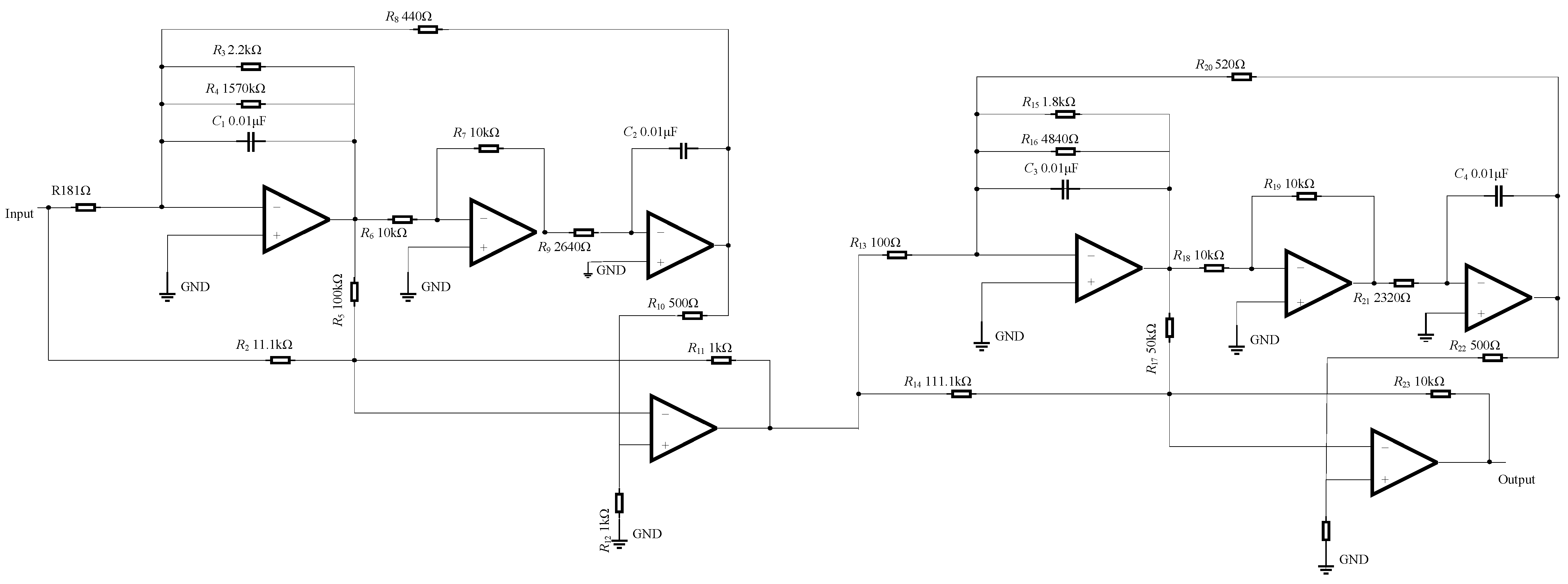
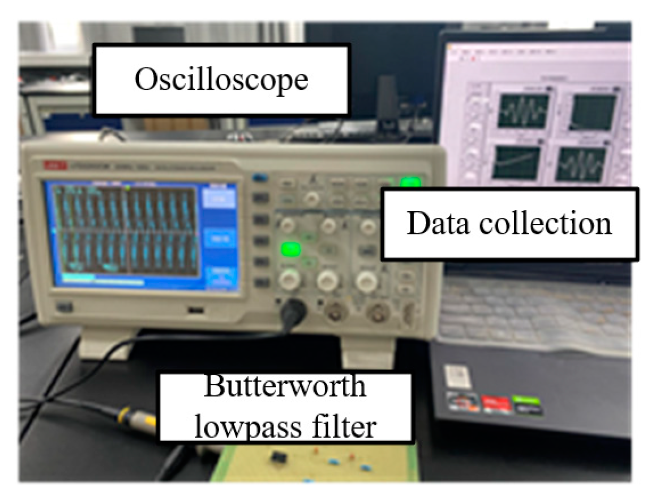
In this paper, the effectiveness of the proposed method is verified through diagnostic experiments on a real analog circuit, specifically the Butterworth low-pass filter shown in
Figure 22. The component parameters used in the physical circuit are detailed in
Figure 5, and the fault modes are set as shown in
Table 1. This allows for testing the performance of the ECA-MI-CNN diagnostic model under different conditions.
The specific steps are as follows:
- (1)
Detect the output voltage and transmit it to LabView with NI acquisition card.
- (2)
Collect 60,000 data points for each fault, resulting in 51,529 sample data points, set the offset to 100, and 80 fault samples can be made, thus totaling 720 samples.
- (3)
Partition training samples and test samples according to the ratio of 7:3.
- (4)
Train and evaluate the model performance.
In the actual experimental verification, 10 independent diagnostic experiments were conducted to reduce the impact of randomness on the results, as shown in
Figure 23. It was found that, under the action of the excitation signal, the original signal in the real environment is inevitably affected by noise, environmental factors, and other influences, which results in a slightly longer operating time compared to the simulation experiments and slightly affects the classification results. Therefore, the performance of the proposed model in practical applications is slightly lower than that of the simulation experiments. As shown in
Table 8, the average diagnostic accuracy of the proposed method is 97.32%, significantly higher than CBAM-MI-CNN (94.86%), Squeeze-and-Excitation Network-MI-CNN (94.27%), MI-CNN (88.31%), and traditional CNN (84.29%).
In addition,
Table 8 shows that the ECA-MI-CNN diagnostic model takes the least time (4.93 s), followed by CBAM-MI-CNN and SENet-MI-CNN (5.72 s and 6.27 s), with MI-CNN and CNN taking the longest time (10.06 s and 12.87 s). The experiments demonstrate that the diagnostic performance of the model can be improved by adding the attention mechanism. However, the fully connected layers inside the SENet and CBAM modules result in a higher number of parameters compared to ECA, which explains why CBAM-MI-CNN and SENet-MI-CNN models perform worse than the proposed model in diagnostic performance.
Further analysis reveals that while the CBAM model outperforms SENet in some tasks, it still falls short compared to the ECA model. In CBAM, both spatial and channel attention mechanisms are introduced simultaneously, which helps enhance the feature representation ability. However, due to the complex structure, the computational cost is higher, resulting in greater computational overhead in practical applications. In contrast, ECA simplifies the attention calculation across channels, maintaining strong classification performance while ensuring efficiency. Therefore, the ECA model not only has advantages in diagnostic accuracy but also offers higher computational efficiency, making it a more ideal choice.
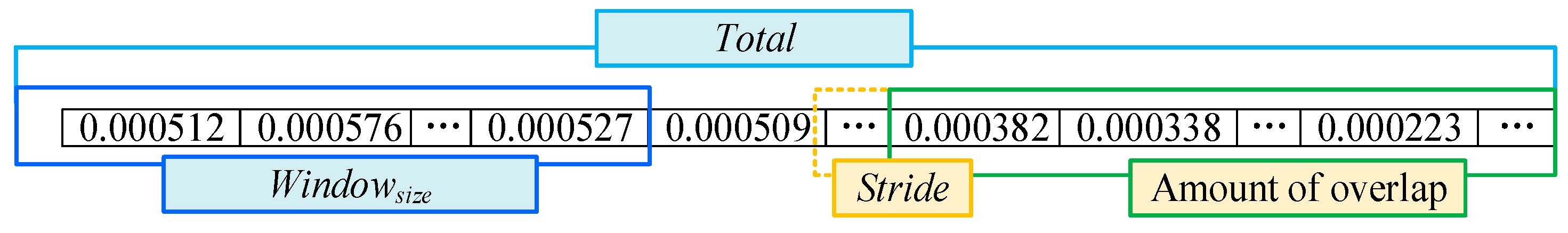
When a circuit is operated for a long time, the circuit parameters are shifted, making the data contain cumulative noise that may affect the diagnostic performance of the network. To verify the robustness of the model, a Butterworth low-pass filter is continuously energized for three days, and then 16,000 sets of circuit fault data are randomly collected, and the ECA-MI-CNN model is enhanced by overlapping sampling to perform signal feature extraction and diagnosis in a noisy background. As can be seen from
Table 9, the average diagnostic accuracy of the ECA-MI-CNN model is 96.83%, which is still better than CBAM-MI-CNN (94.82%), SENet-MI-CNN (93.85%), MI-CNN (85.94%), and conventional CNN (83.81%). The performance of ECA-MI-CNN did not degrade significantly due to the accumulated noise of Butterworth low-pass filter after long time operation. It indicates that ECA has good noise immunity with obvious advantages over CBAM and SENet.
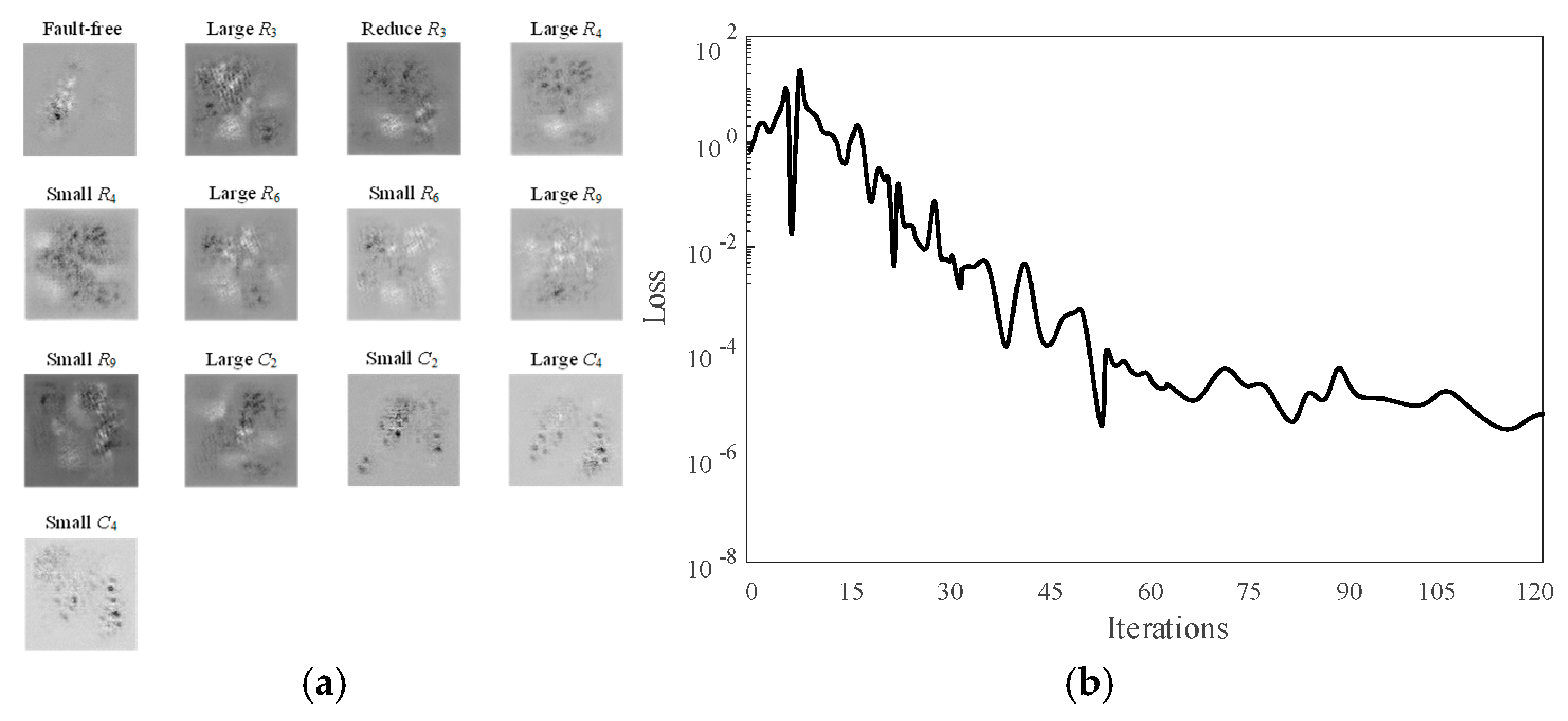
Figure 24 shows a plot of the fault features and feature edge intensities diagnosed by the ECA-MI-CNN model under the condition of long-time operation of the Butterworth low-pass filter, and the edge intensities of the nine features are calculated by the Canny operator. The edge intensity is expressed as the squared error of the partial derivatives, and the higher the peak of the edge intensity, the more distinct the fault feature is. From
Figure 24, it can be seen that the nine fault features of Butterworth low-pass filter have a large degree of difference from each other.
Therefore, it can be proved that the method proposed in this paper can effectively diagnose circuit faults, and can still tap the deep essential features without considering the influence of the environment on the actual circuit signal and the interference of the accumulated noise brought by the long-term operation of the circuit, which has good anti-interference ability and high practical application value, proving the robustness of the model.


