Abstract
In this study, we consider a multi-server priority queueing model with batch arrivals of two types of customers, a finite buffer, and two input finite buffers for storing customers that cannot be admitted for service immediately upon arrival. The transition of a customer from an input buffer to the main buffer can occur after an exponentially distributed time. Customers residing in the input and main buffers are impatient. The four-dimensional Markov chain is used to describe the dynamics of the system under consideration. It is analyzed via the derivation of its generator and providing an effective algorithm for computing its steady-state probabilities. Formulas for calculating the system’s major performance metrics are established. Numerical results demonstrating the suggested methods’ viability and the effect of variation of transition rates of customers from the input buffers are presented.
MSC:
60K25; 60K30; 68M20; 90B22
1. Introduction
Mathematical modeling of many real-world objects can be implemented using the tools provided by queueing theory as the branch of applied probability theory. Initially, queueing theory was developed on the assumption that so-called customers who receive service in a queueing system are statistically homogeneous and have equal importance for the system. However, there are many real-world objects for which this assumption does not hold true. Customers can be categorized into several types. The customers of different types can require different amounts of resources or time for their service. Customers can have different requirements for the indicators of the quality of service and different financial, social, etc., values for the system. In such a situation, it sounds reasonable to differentiate the rate of access, the speed, or the quality of service provided to different types of customers.
One of the well-proven methods for such a differentiation is the assignment of different priorities to different types of customers. Customers having higher priority are better treated in the system: they have easier access to the servers and buffers as well as the first choice after a busy server becomes available.
1.1. Brief Literature Survey
Priority queue analysis has already been the subject of a large body of literature since the early books [1,2,3,4,5]. Various types of priorities are examined in the literature, including preemptive, non-preemptive, mixed, static, dynamic, changing, and accumulating priorities. As recent papers containing more references to the relevant literature and examples of real-world applications, we mention [6,7,8]. Among the wide range of practical applications, the following two popular ones nowadays can be mentioned especially. They are the various applications in telecommunications, e.g., in analyzing the performance of mobile communication networks with handover customers and in cognitive radio systems and healthcare systems, e.g., hospital intensive care unit management, in particular the triage of patients. In this paper, we restrict ourselves to the priority queueing models with two types of customers.
Setting priorities is a very delicate issue because giving more priority to one type of customer inevitably entails the deterioration of service conditions for another type. Therefore, it is necessary to find a reasonable trade-off between the interests of two types of customers and their value or social importance.
In case one type of customer is essentially more important and valuable, evidently the preemptive priority can be provided to this type. This kind of priority supposes that customers of non-priority type do not have any chance to enter service until the moment when a priority customer has been served by one of the servers and no priority customers are waiting. Additionally, when a priority customer shows up while all servers are occupied and some of them are serving non-priority customers, the priority customer begins service, and one non-priority customer is pushed out.
In case one type of customers is more important and valuable but the difference in the values is not very essential, the non-preemptive priority can be used. In contrast to the preemptive priority, service interruption of a non-priority customer at the moment of the priority customer arrival is not allowed.
Sometimes, the importance and value of one type of customer over another one are less essential than in the previously mentioned cases, and the prohibition on non-priority customers (probably already waiting for a long time) entering service until all waiting (probably just arrived) priority customers enter service looks discriminatory and unfair. In such a situation, the mentioned schemes for a priori priority providing may not be flexible enough. Here, we propose and discuss a variant of more flexible provision of advantage to one type of customer. It is realized via the preliminary delay of arriving customers in separate dedicated buffers of a finite capacity and different speeds of customer transition to the main buffer in which customers wait for service beginning when all servers are busy. Such a delay offers some chance to long-waiting non-priority customers to overtake recently arrived priority customers and improves the fairness in access to service.
The mathematical model of the system with such a mechanism of advantage providing was considered in paper [9] for a single-server system and in [6] for a multi-server system. The main buffer was assumed to be infinite, and the possibility of pushing out the customer from the input finite buffer to the main buffer when the finite buffer is full at the next customer arrival was suggested. This was performed to avoid the arriving customer’s loss due to the finite buffer overflow. Customer loss can happen only due to the too-long stay of a customer in a finite or the main buffer, i.e., due to the impatience of customers. Impatience is an important phenomenon, see [10], that has to be carefully taken into account, aiming to adequately model a real-world object. In ref. [11], a recent survey devoted to queueing systems with impatient customers is presented. Very recent papers in this subject are [12,13,14,15,16].
In refs. [6,9], the marked Markov arrival process (), see, e.g., [17], is assumed to define the arrival flow. This is an extension of the more well-known Markov arrival process (), see [18,19,20,21,22], to the case of heterogeneous customers. By taking into account the and rather than the stationary Poisson process, the mathematical model’s suitability for a real-world item is fundamentally increased. The and much better fit the realizations of many real-world processes that can be available as files containing time stamps that record arrival moments. When the inter-arrival time in the actual arrival process exhibits a high variance and a positive correlation, there can be significant inaccuracies in performance characteristics evaluation and assessing the resources needed for the system’s correct operation when the stationary Poisson process is used as the model of the actual arrival process.
1.2. Contributions of This Paper
Compared to the fairly general model examined in [6], the queueing model examined in this study contains the following two key differences and may have promising real-world applications.
- The first one consists of the assumption that customers can arrive not one by one but in batches of a random size. A customer batch arrival is typical for various real-world systems, including telecommunication systems where the transmitted information is divided into smaller units, e.g., packets, and emergency rooms in hospitals where a whole group of patients can appear at the same time due to an accident occurring. The possibility of batch arrivals is taken into account via consideration of the batch marked Markov arrival process (), see, e.g., [20], as the model of arrivals to the system.
- The second one is the assumption that the main buffer has not infinite but finite capacity. This assumption is more realistic for the majority of real-world systems. This assumption makes it impossible to push out the customers from the input buffers to the main one when both the input buffer and the main buffer are overflowed. Therefore, while the customer loss is possible in [6] only due to the impatience, in the considered model customer loss can also occur at the customer arrival moment due to the buffer overflow. The whole group of customers can be lost at the same moment due to the batch arrivals. Thus, to reduce the likelihood of customer loss, which is higher than in the model from [6], the problem of optimal choice of capacities of the buffers and the transition rates of customers from the input buffers to the main one becomes crucial, and it can be solved based on the results of the analysis implemented in this paper.
The listed distinctions essentially complicate the system analysis since the handling of an arbitrary arriving customer can be different depending on the type of customer, the size of a batch in which the customer arrives, the number of idle servers, the occupancy of the respective input buffer, and probably the occupancy of the main buffer. This diversity of possible scenarios of the customer handling implies more technical difficulties in the mathematical description of the system and analysis of the corresponding random process.
1.3. The Outline of the Presentation
The structure of the paper is as follows. The operation of the queueing system with two types of customers, two dedicated input finite buffers, and the finite main buffer is explained in Section 2. The definition of a four-dimensional continuous-time Markov chain () that describes the system’s operation is the focus of Section 3. The main result here is the derivation and proof of the generator of this Markov chain, the entries of which carefully account for all variants of the chain transitions during the infinitesimally small time interval. This generator is the block upper Hessenberg matrix with all zero blocks above the finite number of diagonals above the main diagonal. This makes it possible to simplify the existing technique for solving the equilibrium equations for the vectors of invariant probabilities. In Section 4, formulas for calculating system performance metrics are provided, along with proofs for some of them. Section 5 provides an example of the algorithms’ implementation for computing invariant probabilities and performance metrics. A problem of optimal selection of customers’ transition intensities from the input buffers to the main buffer is also considered. A short Section 6 concludes the paper and briefly touches on the possible directions for future research.
2. Description of the System Under Study and Its Parameters
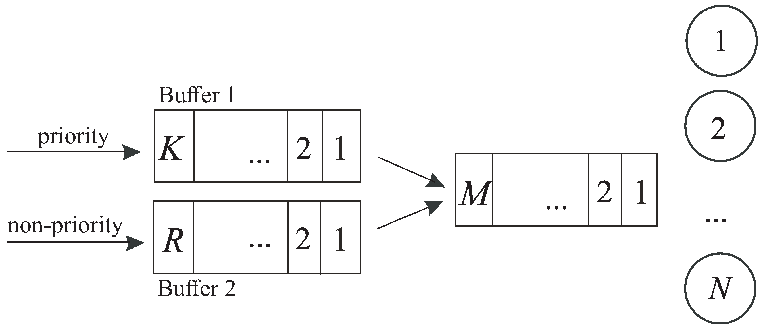
We consider the queueing system that consists of a service device with N identical servers, the finite main buffer of capacity and two input buffers: Buffer 1 and Buffer 2. The capacity of Buffer 1 is equal to K and the capacity of Buffer 2 is equal to . Figure 1 depicts this queueing system’s topology.
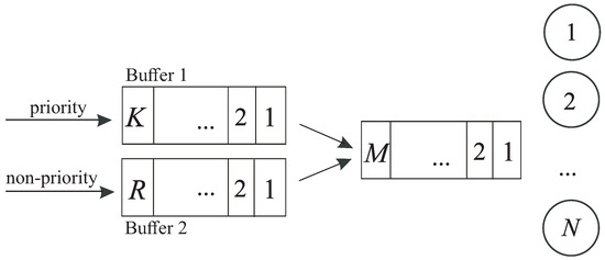
Figure 1.
Topology of the system under consideration.
There are two types of customers entering the considered system in groups. We assume that the maximum size of a group of customers of the first (second) type is limited by parameter . We assume that i.e., the maximum sizes of the batches, do not exceed the capacities of the corresponding dedicated buffers. We denote .
The arrival flow is modeled by the directed by an underlying process . This process is an irreducible continuous-time with the finite state space . The transitions of this chain are defined by the square matrices of size W as follows:
The intensity of the leaving state , is the module of the th diagonal element of the matrix
The intensities of the transitions without the generation of groups of customers are the non-diagonal elements of matrix
The intensities of the transitions with the generation of a group of type-l customers are the elements of matrix
The generator of the has the form
Above, we use the denotation like This means that
Let us represent the vector of stationary probabilities of the states of the by which is the solution to the system
Note that defines a zero row vector and is a unit column vector.
The average arrival rate of customers of type is determined as
The average rate of customers is defined as
For more information on , see, for example, [20].
If the number of idle servers at the moment of arrival of a group of customers of any type is greater than or equal to the size of this group, then all customers from this group start receiving service without visiting any buffer.
If the number of idle servers is lesser than the size of the group, then part of the group of customers of the lth type occupies the free servers and starts service, and the remaining part is placed in Buffer l, , dedicated for storing the lth type customers.
When all servers are occupied at the moment of arrival of a group, then the received customers are placed into the buffer dedicated for their type. Moreover, if there is not enough space there, then part of the customers from the head of the queue proceeds to the main buffer, but no more than the number of free places in the main buffer. Those arriving customers for whom there is not enough space are lost. This implies that we take into account the discipline known as partial admission. Analogously to the analysis below, the alternative disciplines, such as complete rejection (since the entire group is rejected if not all arriving customers can be admitted to the system) or complete admission (since the entire group is accepted if at least one arriving customer can be admitted), can be examined independently.
A type l customer resides in Buffer l for exponentially distributed time with parameter . After this time, the customer tries to enter the main buffer. If the main buffer is full, the customer continues to wait for service in Buffer l. It makes another attempt to leave Buffer l after exponentially distributed time with the same parameter After moving to the main buffer, both types of customers become identical and are served according to the FIFO discipline.
Type-1 customers have priority over type-2 customers. This means the following. The released server serves the first customer from Buffer 1, if any, if the main buffer is empty at the moment of service completion. Only in the case of empty Buffer 1 the first customer from Buffer 2 can be chosen for service. If all buffers are empty, the server waits until a group of customers of any type enter the system, and the server has an opportunity to start providing service.
In addition, the priority of customers of the first type over the second one may be granted by assuming that the rate of the transition of customers of the first type from the input buffer to the main buffer is greater than the rate for the second type of customers and also by choosing a larger capacity of the input buffer for priority customers to reduce the chance of customer loss.
Customers waiting in the buffers are impatient. The customer’s patience time in Buffer l has an exponential distributed time with the intensity , The customer’s patience time in the main buffer has an exponential distributed time with the intensity , A customer departs the system without receiving any service once its patient time has passed (is lost).
The service time of a customer has an exponential distribution with the parameter
In order to compare the quality of the system’s operation under the many variants of the system’s parameters, it is important to examine the system’s performance metrics under each fixed variant. Below we assume that all parameters of the model listed in this section are fixed.
3. Analysis of the Random Process Describing the Behavior of the System
Since the current state of the system is defined by several entities, including the number of busy servers, the number of customers in the main buffer, Buffer 1 and Buffer 2, and the state of the underlying process, there are different ways for constructing the stochastic process that specifies the behavior of the system. We decided to proceed with analysis as follows.
We let
- be the number of customers in the main buffer and on servers;
- be the number of customers in Buffer 1;
- be the number of customers in Buffer 2;
- be the state of the arrival process
- at time
Then, it is easy to see that the process with state space
is an irreducible continuous-time .
In accordance with established methods for analyzing these types of chains, such as [23], we list the states of the under consideration in lexicographic order and designate as level i the collection of states with the value i of the component We denote by Q the generator of the
Theorem 1.
The matrix Q has the following block upper-Hessenberg structure:
where non-zero blocks contain the intensities of the transition from states of level i to states of level
These blocks are defined as follows:
where
- O is a zero matrix and I is the identity matrix, the size of which can be specified by a subscript;
- ⊗ means the operation of the Kronecker product of matrices, see, e.g., [24];
- is the matrix with non-zero entries ;
- is the matrix with non-zero entries
- is the matrix with non-zero entries and ;
- is the matrix with non-zero entries and ;
- is the diagonal matrix with the diagonal entries
- is the matrix with a single non-zero entry ;
- is the square matrix of size n with non-zero entries ;
- is the row vector of size n of form
- is the row vector of size if , and of size if with non-zero entries
- is the matrix with a non-zero entry ;
- is the matrix with a non-zero entry ;
- is the matrix with non-zero entries ;
- is the matrix with non-zero entries ;
- is equal to 1 if A is true and to 0 otherwise.
Proof.
The theorem’s proof is based on analyzing the intensities of every possible transition of the in a negligible amount of time.
The block upper-Hessenberg structure of Q is due to customers entering the system in batches and leaving it (finishing servicing or reneging due to impatience) only one at a time. Also, since no more than customers can enter the system in the considered simultaneously, the blocks are zero blocks for
First, let us examine blocks form.
Since Q is a generator, its diagonal elements are negative. The modules of these entries are the intensity of leaving its states. Leaving can occur due to the following:
- (1)
- the process leaves its current state with the intensities specified by the absolute values of the diagonal elements of the matrix if or the matrix if
- (2)
- a server finishes service. The corresponding intensities are the diagonal elements of the matrix if or the matrix if
- (3)
- a customer leaves Buffer 1 due to impatience. The corresponding intensities are defined by the matrix
- (4)
- a customer from Buffer 1 transits to the main buffer. The rates of this event occurrence are defined by the matrix
- (5)
- a type-2 customer leaves Buffer 2 due to impatience. The rates of this event occurrence are defined by the matrix
- (6)
- a type-2 customer transits to the main buffer. The intensities of this event are defined by the matrix
- (7)
- a customer from the main buffer leaves the system due to impatience. The intensities of occurrence of this event are defined by the matrix
Off-diagonal elements of blocks define the transition intensities within level These intensities are as follows:
- (1)
- off-diagonal elements of the matrix if or if when the arrival process transits to another state with no customers generating;
- (2)
- elements of the matrix when a group of type-1 customers arrives and is admitted to Buffer 1. In the case when (all servers are busy and the main buffer is full), some of the customers of the group that did not have enough space in Buffer 1 may be lost; therefore, such intensities are given by elements of the matrix
- (3)
- elements of the matrix when a group of type-2 customers arrives and is admitted to Buffer 2 and the elements of the matrix when
- (4)
- elements of the matrix when a customer leaves Buffer 1 due to impatience;
- (5)
- elements of the matrix when the customer leaves Buffer 2 due to impatience;
- (6)
- elements of the matrix , when at the end of service there are no customers in the main buffer, and at least one of Buffers 1 and 2 is not empty, and one of the customers from one of these buffers starts service.
Now, let us explain the form of the blocks These blocks contain the transition intensities when the number of customers in the main buffer or being served decreases by one.
Such transitions are possible if service is completed (the intensities are the elements of the matrix if or if ), and if an impatient customer leaves the main buffer (transition intensities are the elements of the matrix ). The transition from level N to level is possible only if the number of customers in all buffers is equal to zero and service in one of all busy servers is completed. Note that such a transition leads to a reduction in the state space of the . This explains the form of the block Here, the vector indicates that Buffer 1 and Buffer 2 are empty.
After that, we describe the structure of the blocks , which establish the intensities of the transitions when the number of customers in service and in the main buffer is changed from i to .
If at the arrival of a group of m customers there are free servers and their number is greater than or equal to m, then all customers occupy free servers and begin service. The intensities of transitions of the arrival process at such arrival epoch are the elements of the matrix if of the matrix if , and of the matrix if
If during an arrival epoch there are free servers but the group size is greater than the number of free servers, then part of the group occupies all free servers and the remaining customers join the corresponding buffer of their type and await transfer to the main buffer or to a server. The corresponding intensities are specified by the matrix for customers of the first type and by the matrix for customers of the second type.
If all servers are busy at the moment when a group of customers arrives and the number of places in the corresponding buffer is lesser than the size of the received group, then some of the customers are placed in the buffer of their type and the remaining part moves to the main buffer. If the number of places in the main buffer is sufficient to accommodate the entire remaining part of the customers, then the corresponding intensities are the elements of the matrix for customers of the first type and the matrix for the second type. Otherwise, some of the customers that do not have enough space are lost, and the corresponding intensities are given by the matrix for type-1 customers and by the matrix for type-2 customers.
The transfer of a customer from any of the input buffers may also result in an additional customer being added to the main buffer, increasing the number of customers by one. The intensities of the transitions caused by customer transition from Buffer 1 are defined by the matrix and the respective transitions from Buffer 2 are defined by the matrix which explains the appearance of these summands in the expression for blocks
Thus, we obtain the form of all non-zero blocks
Theorem 1 is proven. □
Due to the irreducibility of the and the finiteness of its state space, the stationary probabilities of the chain states are defined as the following limits:
existing for any set of the system parameters.
Again, following existing traditions of analysis of such kinds of chains, we build the row vectors of these probabilities as
The vectors can be found by solving the following system:
The number of equations of this system is equal to and can be large. E.g., in the numerical example presented below, it is equal to 44,989. Therefore, the computation of the stationary probability vectors as a solution of System (2) is not an easy task, and specific Structure (1) of generator Q has to be effectively taken into account to speed up the computations. If the customers can arrive only one by one, i.e., , the generator is the block tridiagonal matrix, and the chain belongs to the class of Quasi-Birth-and-Death processes, see, e.g., [23]. The problem of solving System (2) is extensively addressed in the existing literature. The case is more complicated and weakly analyzed in the case of a finite state space of the chain.
A suitable algorithm for solving System (2) with the matrix Q, which is not the block tridiagonal one, was proposed in [25]. In that paper, the queueing system with a finite number of types of customers, the arrival process, and the possibility of the change of the priority of a customer during its waiting in the queue was considered. The generator of the multi-dimensional investigated in [25] has the block upper-Hessenberg structure as the generator of the chain considered in this paper. Because here we assume that the sizes of batches of customers of both types are restricted by the constant, the algorithm proposed in [25] can be simplified. The simplified algorithm is described in Theorem 2 below. It should be noted that this algorithm may be used for any that has the generator of a block upper-Hessenberg structure with a limited number of non-zero diagonals above the main diagonal, not just the concrete examined in this study.
Theorem 2.
The steady-state distribution is calculated as
where the constant and the vectors are found as
The vector is the single solution of system
The non-negative matrices are calculated as
This algorithm is numerically stable because the subtraction operation is not used during any step of its implementation. The inverse matrices that appeared in the algorithm exist.
Once the vectors are computed, it becomes possible to compute various performance characteristics of the system and investigate their dependence on the input parameters.
4. Performance Characteristics Computation
The average quantity of customers residing in the system is
The average quantity of occupied servers is
The average quantity of customers residing in the main buffer is
The average quantity of customers residing in Buffer 1 is
The average quantity of customers residing in Buffer 2 is
Formulas (3)–(7) are evidently derived as expectations of the listed quantities, which are the discrete random variables with probability distributions given by quantities
The output flow rate of successfully serviced customers is
Formula (8) evidently follows from the formula of total probability.
The probability of losing an arbitrary customer of the first type from Buffer 1 due to impatience is
The probability that an arbitrary customer will be lost from Buffer 1 due to impatience is
The loss probability of an arbitrary customer of the second type from Buffer 2 due to impatience is
The loss probability of an arbitrary customer from Buffer 2 due to impatience is
The probability of losing an arbitrary customer from the main buffer due to impatience is
Formulas (9)–(13) are clear as the ratios of the rates of the flow of the lost customers to the rate of the corresponding arrival flow.
The probability of losing an arbitrary customer is
Here, is the share of successfully serviced customers, and correspondingly is the share of the lost customers.
The probability of losing an arbitrary customer of the first type at the entrance to the system due to insufficient space in the system is
Proof.
We suppose that if an arbitrary (tagged) customer arrives within the group consisting of m customers, then it is assigned number j in the group with probability The customers of the group are admitted to the system according to their numbers. In case of the deficit in the capacity of the system, the corresponding number of customers having the maximal numbers are lost first. It is known [20] that, under the fixed states of the underlying process of the , probabilities of an arbitrary customer of the first type arrival within the group consisting of m customers are given by the column vector Some customers of this group can be lost at the entrance to the system when the sum of the numbers of customers in the main buffer and service is i and the number k of customers in Buffer 1 is greater than The probability that namely the tagged customer will be lost is equal to Thus, applying the formula of total probability (by account of the probabilities of all values of i and k for which the loss is possible), we obtain Formula (15). □
The probability of losing an arbitrary customer of the second type at the entrance to the system due to insufficient space in the system is
The probability of losing an arbitrary customer at the entrance to the system due to insufficient space in the system is
Formula (17) evidently follows from the formula of total probability.
Remark 1.
The following equalities are valid:
and
The fulfillment of these equalities can be used to control the accuracy of the implementation of the calculation of the vectors and the performance measures of the system.
The probability that an arbitrary group of customers of the lth type will begin service as soon as it arrives is
Here, is the rate of arrival of batches of the lth-type customer. It is computed as
The probability that an arbitrary customer of the lth type will begin service as soon as it arrives is
5. Numerical Experiment
In the numerical experiment, we demonstrate the viability of the algorithms for calculating the stationary distribution of the system states and performance metrics. Additionally, we examine the impact of the intensities of transitions and from Buffers 1 and 2 to the main buffer on the primary system performance characteristics. The issue of determining the optimal values for these parameters is also resolved numerically.
The input flow of customers of two types is modeled by a flow defined by the following set of matrices:
The batch size of type-1 customers can be equal to and 4. The batch size of type 2 customers can be equal to and 3.
The average intensity of arrival of customers in this flow is the average intensity of arrival of customers of the first type is the average intensity of arrival of customers of the second type is The correlation coefficient of successive inter-arrival times of customer groups is , and the square of the variation coefficient is . The average intensity of arrival of customer groups of the first type is customer groups of the second type is .
Let us fix the capacities of the input buffers and the capacity of the main buffer be Let the impatience intensities in Buffer 1 and Buffer 2 be and , respectively, and in the main buffer The number of servers is the average service rate by each server is
We vary the intensities and of the transition from Buffer 1 and Buffer 2 to the main buffer in the interval with a step of
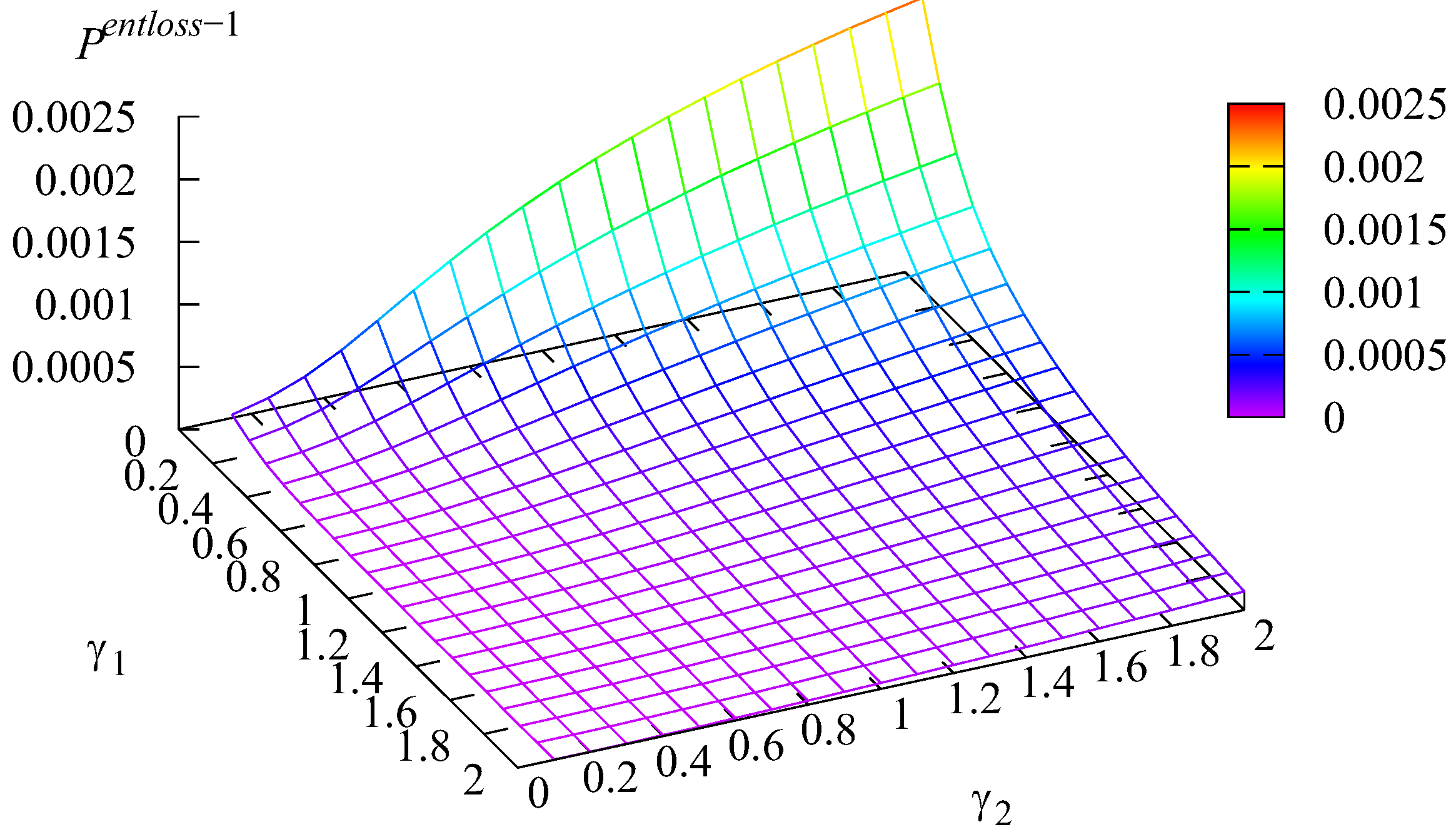
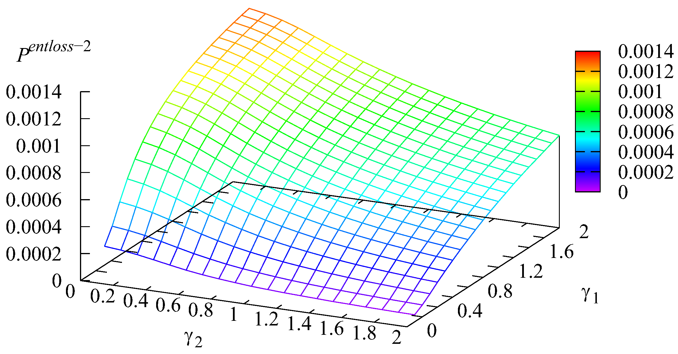
Figure 2 and Figure 3 show the shape of the dependencies of the probabilities and of an arbitrary customer of the first or second type loss at the entrance to the system due to insufficient space in the system.
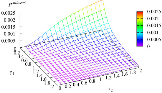
Figure 2.
Dependence of on and .
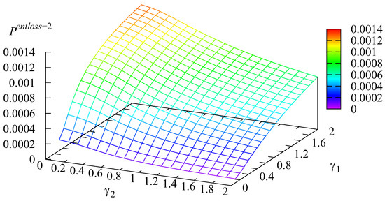
Figure 3.
Dependence of on and .
Figure 2 and Figure 3 confirm the intuitive anticipation that probability is maximal when the transition rate is minimal while the transition rate is maximal , which implies that the customers of type k more quickly transit from the input buffer to the main one. This increases the likelihood that the kth buffer is not overloaded. Figure 2 and Figure 3 quantitatively illustrate this effect.
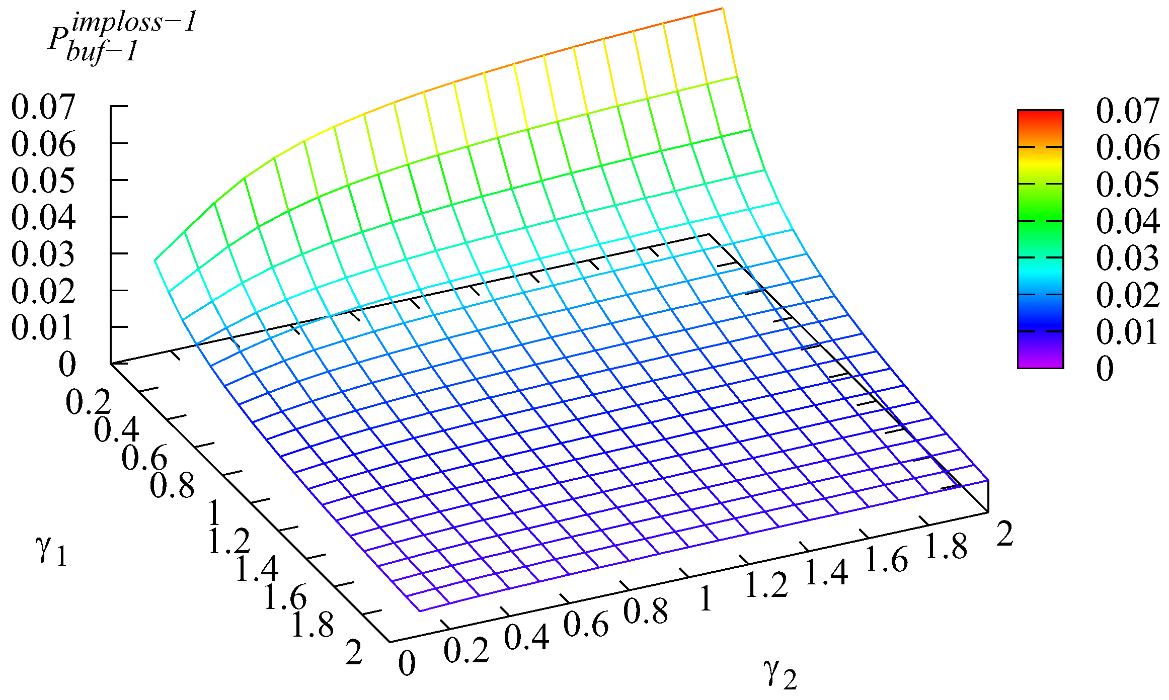
Figure 4 and Figure 5 show the shape of the dependencies of the probabilities and of loss of arbitrary first and second type customers from the corresponding buffer due to impatience on different values of the intensities and
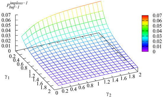
Figure 4.
Dependence of on and .
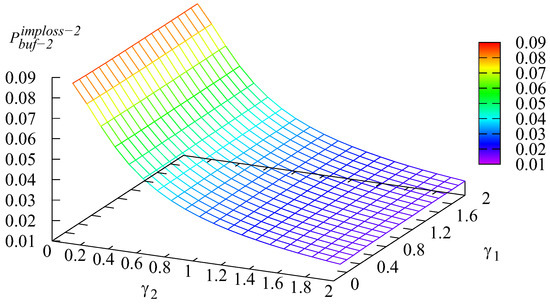
Figure 5.
Dependence of on and .
Figure 4 and Figure 5 show the same tendency as Figure 2 and Figure 3: the higher rate of a customer of some type transitioning to the main buffer implies the smaller loss probability of this type of customer.
The dependence of the probability of loss of an arbitrary customer from the main buffer due to impatience and the probability of loss of an arbitrary customer for different values of intensities and are presented in Figure 6 and Figure 7.
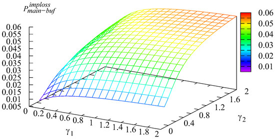
Figure 6.
Dependence of on and .
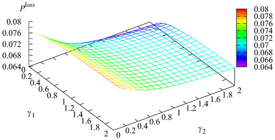
Figure 7.
Dependence of on and .
It is evident from Figure 6 that the probability of loss of an arbitrary customer from the main buffer due to impatience is minimal when both intensities and are small and quickly increases with the growth of these intensities. This is easily explained by the smaller probability of a customer loss in the corresponding input buffer when the transition rate is high. If more customers are not lost in the input buffers, more customers attend the main buffer, which increases the likelihood that a customer from this buffer will be lost due to impatience.
The shape of the surface drawn on Figure 7 matches Figure 2, Figure 3, Figure 4, Figure 5 and Figure 6 with the account of Formulas (17) and (18).
It is demonstrated above that the increase in rate decreases loss probabilities of customers of the kth type. However, this increase in the rate causes the increase in the loss probabilities of customers of another type. Because customers of two types can have different values for the system manager, there arises the problem of the choice of and which provides the maximum for the profit of the manager. Evidently, the profit from providing service to customers increases when fewer customers are lost. The penalty per customer loss depends on the type of customer (it is higher when the valuable customer is lost) and on the stage of the customer processing in the system at which it is lost: arrival to the input buffer, waiting in this buffer, and waiting in the main buffer.
Let us fix the following criterion of quality of the system operation:
where is the penalty for losing one customer of type l from Buffer is the penalty for not accepting one customer of type l due to system overflow, c is the penalty for losing one customer from the main buffer per unit of time. The cost criterion specifies the system losses per unit of time.
Let us find the optimal values of and that provide the minimum of this criterion.
Let us fix the following values of cost coefficients:
Since customers of the first type are priority ones, the penalties for their loss are chosen to be greater than for the loss of customers of the second type.
The surface showing the dependence of the cost criterion on the transition intensities and is presented in Figure 8.
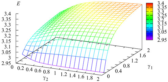
Figure 8.
Dependence of E on and .
From Figure 8, we can conclude that in the example under consideration, the optimal value of the criterion is with That is, in this case, to minimize the value of the criterion, it is necessary to fix the minimum permissible intensity value and the value
Using Wolfram Mathematica 12.2, calculations were performed on a Lenovo notebook equipped with an Intel(R) Core(TM) i7-1165G7 2.80 GHz and 16 GB of RAM. Running time for calculating performance measures and the cost criterion’s optimal value, , was 10,279 s, i.e., 26.7 s for each of 400 considered points This time may be considered moderate, taking into account the size of about 45,000 of the system of equations for the vectors of the stationary probabilities and the relatively low power of this notebook. If we consider the change in not from 0.1 but from 0, then the optimal value of the criterion is with That is, with the given data, customers of the first type must be prohibited from moving to the main buffer, and the system itself must take these customers from Buffer 1 when some server is idle, despite the fact that the penalties for losing customers of the second type are lesser than for the loss of customers of the first type. This can be explained by the following facts: (i) the customers of the first type have the essential advantage over the customers of the second type because the second-type customer can be picked up by an idle server only if the queue of the first-type customers is empty; (ii) in the considered example, customers of the second type are more impatient, i.e., , and it makes sense to more quickly transfer them from the input buffer to the main one to reduce the chance of their loss in the input buffer.
6. Conclusions
A new scheme of providing flexible priority service in the system with two types of customers arriving in the flow described by the batch marked Markov arrival process is proposed.
Priority to one of the types is provided via the preliminary storing of customers in separate input dedicated buffers of a finite capacity, different capacities of these two buffers, different rates of customer transfer from the input buffers to the main buffer of a finite capacity, and the privilege of picking up the customer from a corresponding input buffer when the main buffer is empty at service completion by one of the multiple servers of the system.
Given the fixed configuration of the system and the rates defining customer arrival, transition, impatience, and service, the behavior of the system is described by the four-dimensional . The generator of the chain is derived, and the numerically stable algorithm for computing the stationary distribution of the chain is offered. Analytic expressions for various performance indicators of the system are derived, and their behavior as functions of transition rates to the main buffer is explored.
The proposed scheme is essentially more flexible, e.g., compared to the standard priority discipline. In particular, the standard non-preemptive priority for the first type is obtained from the considered one if the rate of transitions from the buffer storing the second type of customers is set to be zero. The increase in this rate smoothly decreases time till the beginning of service of non-priority customers and increases the fairness of the access discipline. Results can be extended to the case of more general service time distribution, namely phase type distribution; see, e.g., ref. [23] for definition and details. Various types of unreliability of the servers and the existence of so-called negative customers can be incorporated as well. Group service of customers and buffers clearance can be analyzed.
Author Contributions
Conceptualization, A.D., O.D. and A.M.; methodology, A.D., O.D. and A.M.; software, O.D. and S.D.; validation, O.D. and A.M.; formal analysis, A.D., S.D. and O.D.; investigation, S.D., A.D., O.D. and A.M.; writing, original draft preparation, S.D., A.D., O.D. and A.M.; writing, review and editing, investigation, A.D., O.D. and A.M.; supervision, S.D.; project administration, A.D. All authors have read and agreed to the published version of the manuscript.
Funding
This research received no external funding.
Data Availability Statement
The original contributions presented in this study are included in the article. Further inquiries can be directed to the corresponding author.
Conflicts of Interest
The authors declare no conflicts of interest.
References
- Jaiswal, N.K. Priority Queues; Academic Press: New York, NY, USA, 1968. [Google Scholar]
- Takagi, H. Queueing Analysis: A Foundation of Performance Evaluation, Volume 1: Vacation and Priority Systems; Elsevier Science Publishers: Amsterdam, The Netherlands, 1991. [Google Scholar]
- Kleinrock, L. Queueing Systems, Volume 2: Computer Applications; Wiley: New York, NY, USA, 1976. [Google Scholar]
- Gnedenko, B.V.; Danielyan, E.A.; Dimitrov, B.N.; Klimov, G.P.; Matvejev, V.F. Priority Queueing Systems; Moscow State University: Moscow, Russia, 1973. (In Russian) [Google Scholar]
- Bronstein, O.I.; Dukhovny, I.M. Priority Service Models in Information and Computing Systems; Science: Moscow, Russia, 1976. [Google Scholar]
- Samouylov, K.; Dudina, O.; Dudin, A. Analysis of Multi-Server Queueing System with Flexible Priorities. Mathematics 2023, 11, 1040. [Google Scholar] [CrossRef]
- Lee, S.; Dudin, A.; Dudina, O.; Kim, C. Analysis of a priority queueing system with the enhanced fairness of servers scheduling. J. Ambient. Intell. Humaniz. Comput. 2024, 15, 465–477. [Google Scholar] [CrossRef]
- Yang, H.; Fu, J.; Wu, J.; Zukerman, M. A study of a loss system with priorities. Heliyon 2024, 10, e36109. [Google Scholar] [CrossRef] [PubMed]
- Dudin, S.; Dudina, O.; Samouylov, K.; Dudin, A. Improvement of fairness of non-preemptive priorities in transmission of heterogeneous traffic. Mathematics 2020, 8, 929. [Google Scholar] [CrossRef]
- Boots, N.K.; Tijms, H. A multiserver queueing system with impatient customers. Manag. Sci. 1999, 45, 444–448. [Google Scholar] [CrossRef]
- Sharma, S.; Kumar, R.; Soodan, B.S.; Singh, P. Queuing models with customers’ impatience: A survey. Int. J. Math. Oper. Res. 2023, 26, 523–547. [Google Scholar] [CrossRef]
- Kumar, V.; Upadhye, N.S. Modeling and simulation of first-come, first-served queueing system with impatient multiclass customers. Oper. Res. 2025, 25, 1–37. [Google Scholar] [CrossRef]
- Pan, Y.Y.; Zhang, J.C.; Liu, Z.M. Equilibrium Behavior in a Two-Stage Reneging Queue with Impatient Customers. J. Oper. Res. Soc. China 2025, 1–25. [Google Scholar] [CrossRef]
- Ayyappan, G.; Gurulakshmi, G.A.A. Analysis of MAP/PH/1 queueing system with discarding customers having imperfect service, single vacation, feedback and impatient customers. Int. J. Math. Oper. Res. 2024, 29, 411–440. [Google Scholar] [CrossRef]
- Bu, Q. Transient Analysis for a Queuing System with Impatient Customers and Its Applications to the Pricing Strategy of a Video Website. Mathematics 2024, 12, 2030. [Google Scholar] [CrossRef]
- Varshney, S.; Acharya, M.; Kanjibhai, Z.J.; Pushkarna, M.; El-Shafai, W.; Zaitsev, I. Economic and Sensitivity Analyses of Controllable Queues with Customer Feedback and Impatience Using Markovian Modeling. J. Math. 2025, 2025, 9648114. [Google Scholar] [CrossRef]
- He, Q.M. Queues with marked customers. Adv. Appl. Probab. 1996, 28, 567–587. [Google Scholar] [CrossRef]
- Chakravarthy, S.R. Introduction to Matrix-Analytic Methods in Queues 1: Analytical and Simulation Approach—Basics; ISTE Ltd.: London, UK; John Wiley and Sons: New York, NY, USA, 2022. [Google Scholar]
- Chakravarthy, S.R. Introduction to Matrix-Analytic Methods in Queues 2: Analytical and Simulation Approach—Queues and Simulation; ISTE Ltd.: London, UK; John Wiley and Sons: New York, NY, USA, 2022. [Google Scholar]
- Dudin, A.N.; Klimenok, V.I.; Vishnevsky, V.M. The Theory of Queuing Systems with Correlated Flows; Springer Nature: Cham, Switzerland, 2020; ISBN 978-3-030-32072-0. [Google Scholar]
- Lucantoni, D. New results on the single server queue with a batch Markovian arrival process. Commun. Stat. Stoch. Model. 1991, 7, 1–46. [Google Scholar] [CrossRef]
- Gonzalez, M.; Lillo, R.E.; Ramirez-Cobo, J. Call center data modeling: A queueing science approach based on Markovian arrival processes. Qual. Technol. Quant. Manag. 2024, 1–28. [Google Scholar] [CrossRef]
- Neuts, M.F. Matrix-Geometric Solutions in Stochastic Models: An Algorithmic Approach; Courier Corporation: North Chelmsford, MA, USA, 1994. [Google Scholar]
- Graham, A. Kronecker Products and Matrix Calculus with Applications; Courier Dover Publications: Mineola, NY, USA, 2018. [Google Scholar]
- Dudin, A.; Dudina, O.; Dudin, S.; Samouylov, K. Analysis of single-server multi-class queue with unreliable service, batch correlated arrivals, customers impatience, and dynamical change of priorities. Mathematics 2021, 9, 1257. [Google Scholar] [CrossRef]

Disclaimer/Publisher’s Note: The statements, opinions and data contained in all publications are solely those of the individual author(s) and contributor(s) and not of MDPI and/or the editor(s). MDPI and/or the editor(s) disclaim responsibility for any injury to people or property resulting from any ideas, methods, instructions or products referred to in the content. |
© 2025 by the authors. Licensee MDPI, Basel, Switzerland. This article is an open access article distributed under the terms and conditions of the Creative Commons Attribution (CC BY) license (https://creativecommons.org/licenses/by/4.0/).