Evaluating Predictive Models for Three Green Finance Markets: Insights from Statistical vs. Machine Learning Approaches

Abstract

As climate change has become of eminent importance in the last two decades, so has interest in industry-wide carbon emissions and policies promoting a low-carbon economy. Investors and policymakers could improve their decision-making by producing accurate forecasts of relevant green finance market indices: carbon efficiency, clean energy, and sustainability. The purpose of this paper is to compare the performance of single-step univariate forecasts produced by a set of selected statistical and regression-tree-based predictive models, using large datasets of over 2500 daily records of green market indices gathered in a ten-year timespan. The statistical models include simple exponential smoothing, Holt’s method, the ETS version of the exponential model, linear regression, weighted moving average, and autoregressive moving average (ARMA). In addition, the decision tree-based machine learning (ML) methods include the standard regression trees and two ensemble methods, namely the random forests and extreme gradient boosting (XGBoost). The forecasting results show that (i) exponential smoothing models achieve the best performance, and (ii) ensemble methods, namely XGBoost and random forests, perform better than the standard regression trees. The findings of this study will be valuable to both policymakers and investors. Policymakers can leverage these predictive models to design balanced policy interventions that support environmentally sustainable businesses while fostering continued economic growth. In parallel, investors and traders will benefit from an ease of adaptability to rapid market changes thanks to the computationally cost-effective model attributes found in this study to generate profits.

1. Introduction

While green equity markets are currently trending among investors and economic policymakers, forecasting their prices and indices accurately is important for their decision-making process. Since 2004, global energy transition investments have been growing as the world shifts from fossil fuels to clean energy. In addition, while this change creates new possibilities for green market investors, many external factors, including oil prices and technology stock prices, complemented by the economic policy uncertainties, affect the outcome of these equities [1]. According to the Organization for Economic Co-operation and Development (OECD), green investments are allocated differently across companies, resulting from a strategic split between direct financing and research and development. While direct financing ensures that capital is readily available for projects and company operations promoting sustainable activities, research and development investments focus on realizing innovations in renewable energy, like solar and wind power, and on improving carbon emission efficiency by waste reduction and by finding ways to capture carbon emissions before they reach the atmosphere. The former approach is low risk, whereas the latter carries a higher risk, as it requires a longer timeframe to yield results and involves uncertainties regarding both the success of the development and market acceptance of the new technologies [2]. Recognizing that green finance reform in industries necessitates a careful balance between integrating new technologies and operational advancements within existing industrial frameworks while maintaining economic growth is no easy feat. A pilot project was initiated in China in 2017 to assess the pros and cons of sustainable industrial development [3]. The results were more favorable in regions with larger economies and where central and local governments demonstrated stronger alignment in policy implementation. In contrast, regions with smaller economies and weaker central-local alignment struggled to maintain industrial advancements. Therefore, it was determined that policymakers play a crucial role in maintaining a balance between industries’ environmental objectives and their economic growth.

Another recent in-depth study conducted on green market indices [4] reveals that a lot of information goes into formulating each one of them. Some indices will only include companies that meet a minimum social and environmental standard with respect to their economic sector. Other indices are formulated on the presumption that only the best-performing companies engaged in Sustainable and Environmental Investment (SRI) across all economic sectors will carry a weight in the computation of a given index. Like all financial market indices, green market indices are intrinsically related to a select group of stock prices, implying that they are mainly driven by supply and demand market forces. As challenging as these forces may be to predict, they depend on complex and complicated factors, notably macroeconomic indices, government policies and regulations, as well as companies’ earnings and profits, and investor sentiment coming from social media [5,6]. Concurrently, the advent of artificial intelligence technology has enabled machine learning (ML) models to emerge and evolve to the extent that they can tackle challenging forecasting tasks that the traditional models of statistics cannot do as effectively.

With multiple factors affecting the value of market equities, the forecasting task in this study will be limited to historical data only. In fact, most stock market prediction studies have approached this task using a single data source of historical stock market values to predict future ones [7]. Certainly, the inclusion of several external factors would better account for the erratic behavior of these time series, such as volatility, fluctuating trends, anomalies, and lastly, noise. This would likely lead to improved prediction accuracy and provide motivation to explore this angle in a future study. Looking briefly at some prominent forecasting models that are driven by single sources of data, the econometric models are notable models. The auto-regressive moving average (ARMA) model, auto-regressive integrated moving average (ARIMA) model, generalized ARMA (GARMA), auto-regressive conditional heteroscedasticity (ARCH), generalized ARCH (GARCH), and state-space models have been around for decades and are still popular among researchers and analysts [8,9,10]. Nonetheless, they present shortcomings when dealing with the volatile and unpredictable nature of equity markets. Soft computing methods such as fuzzy logic (FL), genetic algorithms (GA), and particle swarm optimization (PSO) have enriched the realm of forecasting methods for financial time series data using single-source data and yielding improved accuracy results due to their ability to handle uncertainty and/or their optimization capability [11,12]. In another study, the forecast performances of soft computing-based models of artificial neural network (ANN) and support vector machine (SVM) are compared to multiple linear regression on the S&P 500 stock index, using historical stock index values and other financial and economic variables to predict future index values [13]. It was found that the SVM model performed the best due to its ability to nonlinearly map the training data while still using principles of linear classification, thanks to its Radial Basis Function (RBF) kernel [14,15,16]. Optimal hyperparameter tuning through a grid search was also of crucial importance in yielding high accuracy results for the SVM model.

The most recent developments in predicting green market time series present innovative ideas encompassing notions of decompositions of the time series and hybridization of models and processes. Listed next are six of the latest methods proposed to achieve improved short-term prediction accuracy on such data. Firstly, there is a study on the Chinese low-carbon emission index series DT50, whereby great lengths are taken to accurately predict the volatile time series. A multi-mixing approach is applied on realized volatility measures, where a mixed data sampling implementation strategy provides intraday information and the inclusion of the macroeconomic indicator CEPU (Chinese Economic Policy Uncertainty) [17]. Other studies on forecasting carbon emission index emphasize the need to implement a data preprocessing step in the forecasting task [18]. Indeed, a reliable framework, including either a machine learning or deep learning algorithm, is complemented by a well-defined decomposition method. For instance, implementing at least one decomposition method in the data preprocessing step of complex series helps to extract the surplus of noise. Another study applied an ICEEMDAN (integrated complete ensemble empirical mode decomposition with adaptive noise) method, followed by a second decomposition of VMD (variational mode decomposition) and an SE (Sample Entropy) integration to improve the processing time for improved accuracy for this ensemble model [19]. Secondary decomposition integration is echoed again in two other studies [20,21] to overcome whatever instability remains in a first decomposed series. Lastly, the INGDeepAR (incremental Gaussian deep autoregressive) method is a sixth method that is included in this literary review [22]. It takes another angle on the data preprocessing step to predict carbon prices for a multi-step horizon. The time series are converted to fuzzy information granules by means of the sparrow search algorithm (SSA) to obtain incremental Gaussian nonlinear trend fuzzy granulation. A small finite number of granulations are obtained, for which each one is segmented into three DeepAR networks: trend, periodic, and residual information. The final prediction combines the predictions of a nonlinear trend and residual information.

Achieving higher accuracy through the innovative approaches discussed above comes at the cost of increased computational time. Decomposition methods and hybridization techniques for green finance forecasting rely on complex, resource-intensive algorithms that can be time-consuming. When real-time predictions are required, these advanced methods may not always provide the most efficient solution. In contrast, simpler models, like those examined in this study, offer a more practical alternative for such tasks.

Prediction accuracy in this study is defined by three performance metrics to evaluate the fit of each predictor on the data. Nine forecasting methods recognized for short-term forecasting are analyzed to produce a single-step forecast [23]. The forecasting methods are divided into three distinct groups demarcated by their advantages and limitations, and by their model assumptions, or lack of assumptions, and their unique built-in algorithms: (1) statistical models, (2) exponential smoothing models, and (3) ML methods. The statistical models are characterized by their linearity assumptions and other distribution assumptions. They perform well with small datasets that are stationary. Exponential smoothing models, also known as the “classical” time series models [8]; however, are less stringent with model assumptions and are more data-driven. They are well-suited for short-term forecast horizons. Meanwhile, ML algorithms are capable of handling large and complex datasets characterized by uncertainty, nonlinearity, and non-stationarity, making them compelling predictors to use. They do not rely on statistical parameters nor on any distribution assumptions, but instead they are data-driven [23,24]. Having become a widely popular tool to predict financial time series in the last 25 years [25], Decision Trees remain one of the most used algorithms in ML [26]. It follows that the main objective of this study is to analyze and compare how each of these groups of predictors succeeds in achieving the best prediction accuracy, given their characteristics. Indeed, research in green market indices is a new topic that received no attention in applying statistical models and machine learning techniques for market prediction purposes. Many investors and portfolio managers are becoming interested in investing in such markets, and they need to know which predictive model can generate accurate forecasts. Therefore, the main purpose of the current work is to conduct a comprehensive study used to compare standard statistical models and machine learning for green finance market prediction. As a result, green finance traders and investors would get insight about suitable predictive models that could be implemented to generate profits. To draw general conclusions, all statistical and machine learning models are applied to three different green finance markets. This study also offers explanations for the outcomes obtained, and it explores ways for potential improvements moving forward.

Emphasis is placed solely on historical index values to forecast future ones. Observing that the three index time series exhibit short-term fluctuations, sporadically switching from short-lived segments of exponential increases to exponential decreases over the entire ten-year timeframe, it was thus determined that using seven time lags on each set of daily time series can provide enough valuable historical data to capture the observed short-term patterns and to predict future movements. Further, since the forecasting task is short-term in this study, using seven time lags on the daily time series is a good first step in this analysis, although a more comprehensive approach also including multiple external factors would probably yield more valuable insights [8,27]. Hence, the model features used in this study are solely the seven most recent index values captured to predict the next one. These input variables are for all models, except the exponential smoothing-based models, which use an intrinsic weight decaying algorithm on all past values to capture trends and other time-sensitive patterns [5].

To add robustness to the results found, a comparative analysis is conducted using selected forecasting methods on three different time series from green and sustainability financial markets. The statistical models include simple exponential smoothing, Holt’s method, ETS (exponential model accounting for error, trend, and seasonality through automated selection [28]), linear regression, weighted moving average, and autoregressive moving average (ARMA). The decision tree-based machine learning (ML) methods include the standard regression trees [29], random forests [25], and extreme gradient boosting (XGBoost) [30]. While regression trees are data-driven machine learning models, the Random Forest and XGBoost models are ensembles of regression trees used to better model the data in a more complex framework compared to standard regression trees. The performance of the regression trees, random forest and XGBoost, depends on their respective parameters. Therefore, the second objective of this study is to analyze the robustness of the results found in the single-step forecasts across the nine different models evaluated. Since the exponential smoothing models consistently yield the best prediction accuracy results on all three green finance markets, this provides a good degree of certainty in the conclusions drawn in this study on the best performing models for short-term forecasting.

While many studies have wallowed in the comparison of prediction accuracy obtained from statistical methods and other classical time series models to popular machine learning methods, this paper provides an innovative examination on how these traditional models outperform the decision tree-based machine learning methods on three green market time series. The exceptional performance of the exponential-based models may not be immediately apparent from the line graphs presented in this study. However, novel insight is gained on the performance of these models thanks to the inclusion of horizon charts in this comparative study. The charts’ close-up viewpoint highlights the advantages of using exponential-based models to fit the three time series. In this study, the horizon charts are presented in a grid format sorted by model and by index time series, all while examining each model’s performance over the entire validation period relative to the observed time series. Varying shades of color bands visually depict the relative differences between actual and predicted values, with the exponential-based models exhibiting the smallest absolute relative differences.

From an economic perspective, the expected results are far-reaching. Determining more accurate forecasting models from a blend of common statistical models and ensemble learning-based ML models like Random Forest and XGBoost models would enable managers and traders to improve pricing strategies, hedging tactics, and eventually result in more profitable decision-making. For instance, they can find the appropriate model to be implemented to generate profits in such new and fluctuating markets while reducing risk and maximizing returns.

The contributions of our study are as follows:

• Focusing on forecasting prices of green finance and clean energy markets.
• Considering three different markets for better generalization of the results.
• Comparing and examining the performance of statistical and regression tree-based ML models in forecasting such volatile and attractive markets for investors and policymakers, while considering each model’s practical usability, its scalability, and its deployment feasibility for real-time decision-making.
• Comparing the performance of ensemble models, namely XGBoost and random forests, to the standard regression trees.
• Explaining the simulation results through an in-depth analysis of each model’s performance at single time intervals within the validation dataset to ultimately better understand the managerial implications of the findings.

Descriptions of the models selected for this analysis, on the three exploited time series, and on the performance evaluation measures used are presented in Section 2. The results obtained per time series are reported in Section 3. This study is finally concluded with insightful interpretations and a discussion in Section 4 and concluding remarks in Section 5.

2. Materials and Methods

Three categories of models are defined based on their commonalities: (1) the traditional statistical models, based on linear assumptions, (2) the classical time series models from the family of exponential smoothing models, and (3) the ML models that are decision tree-based for quantitative data (i.e., regression trees). They are presented next.

2.1. Statistical Models

2.1.1. Multiple Linear Regression

By using the lagged values of the last seven index values (i.e., $y_{t-7}, \dots , y_{t-1})$ as features to predict the current index value at time t (i.e., target, $y_t$). A linear relation is assumed to exist between the independent variables and the target. It is translated into a linear equation with the target variable equated to the independent variables plus an added intercept. This model is easy to interpret as the magnitude and sign of the coefficients provide a direct measure of the relation between each feature (i.e., each independent variable) and the target. This model can be trained to offer high prediction accuracy, but it is prone to perform poorly on unseen data. It is represented by the equation of the form:

$$y_t={\beta }_0+{\beta }_1{y}_{t-1}+\dots +{\beta }_7{y}_{t-7}$$

(1)

2.1.2. Weighted Moving Average

The weighted moving average [31] with 7 periods (i.e., WMA(7)) provides a linear combination of a positive weighting scheme for 7 consecutive observations at a time. Forecasts obtained from this linear method are such that the most recent moving average provides a forecast for the next time period. This approach allows for the smoothing out of any white noise present over 7 observations at a time to capture potential trends. The sum of the weights assigned to each of the 7 observations adds up to 1. The mathematical form for this model is as such:

$$WM{A}_t=w_1{y}_{t-1}+\dots +w_7{y}_{t-7}$$

(2)

where $w_1+w_2+\dots +w_7=1$.

2.1.3. Moving Average Model

The moving average model of the family of Autoregressive Moving Averages models (ARMA(0, q)) [27] is a linear combination of the past q forecast errors used to predict the value at time t. Useful for short-term forecasting, this model is effective in handling the series when it has serial correlation in the forecast errors. Like the linear regression model in (1.1), the ARMA(0, q) model is straightforward and easy to interpret. Applying this model to the original time series for single-step forecasting, it takes on the following form:

$$y_t=\mu +{ϵ}_t+{\theta }_1{ϵ}_{t-1}+\dots +{\theta }_7{ϵ}_{t-7}$$

(3)

where ${ϵ}_t$ is the forecast error term (also known as. “random shock”) of the time series at time t, and where

-

${ϵ}_{t-1},\dots , {ϵ}_{t-7}$ are the 7 consecutive forecast errors of the time series in past time periods t − 1, …, t − 7,

-

μ is the mean value, also known as the level, of the time series,

-

${\theta }_1,\dots , {\theta }_7$ are the parameters of this linear model.

2.2. Exponential Smoothing Models

2.2.1. Simple Exponential Smoothing

The simple exponential smoothing model provides an exponentially weighted moving average scheme on all previously observed values [32]. Made for univariate data model, it is appropriately applied to time series that have no predictable upward nor downward trend direction. The aim of this model is rather to predict the current level of the series. By “smoothing” or averaging past observations in an exponentially decreasing way, the most recent observation is attributed the largest weight of α, for 0 < α < 1, the observation before that is attributed less weight, resulting from the product of $\alpha \left(1-\alpha \right)$, the observation two time periods before it is attributed even less weight, that of $\alpha {\left(1-\alpha \right)}^2$, etc. The result is a forecast for time t derived from a weighted sum of most recent and previous observations with exponentially decreasing weights,

$${\widehat{y}}_{t+1}=\alpha y_t+\alpha \left(1-\alpha \right)y_{t-1}+\alpha {\left(1-\alpha \right)}^2{y}_{t-2}+$$

(4)

This equation is best summarized with the following formula:

$${\widehat{y}}_{t+1}=\alpha y_t+\left(1-\alpha \right){\widehat{y}}_t$$

(5)

2.2.2. Holt’s Model

Holt’s model [33] is a versatile method that offers a linear trend function to an exponential smoothing model. This is achieved by using estimates of smoothing constants for the level and for the slope of the series. The smoothing constants change over time as new observations become available. For a single step ahead forecast, the formula is:

$${\widehat{y}}_{t+1}=l_t+b$$

(6)

where the current level estimate is formulated as $l_t=\alpha y_t+\left(1-\alpha \right)\left(l_{t-1}+b_{t-1}\right)$, and the trend estimate is $b_t=\beta \left(l_t-l_{t-1}\right)+\left(1-\beta \right)b_{t-1}$,

-

$l_t$ is the estimate of the current level at time $t$;

-

$b_t$ is the estimate of the trend at time $t$;

-

$y_t$ is the most recent observation value at time $t$;

-

$\alpha$ is the smoothing constant for level, with $0<\alpha <1$;

-

$\beta$ is the smoothing constant for trend, with $0<\beta <1$.

For Holt’s method with a damped trend, optimal results are obtained with a configuration of α = 0.8074 for the smoothing parameter, β = 0.0546 for the trend smoothing parameter, and ϕ = 0.80 to control the rate at which the trend is dampened over time.

2.2.3. ETS Model

The ETS model is an exponential model that accounts for error, trend, and seasonality through automated selection [28,34] is included in this analysis to see how it compares to the two other exponential models. Driven by a minimum Akaike information criterion (AIC), the ETS model is different for each time series, with variations on the Error (additive or multiplicative) and the Trend (none, additive, additive damped) components, and without a seasonal component.

2.3. Machine Learning Models

2.3.1. Regression Trees

The regression tree is an ML model that uses a supervised learning algorithm to split quantitative, or continuous, data into subsets based on individual features. Able to detect feature interactions, this model can establish potential nonlinear relations in the data, a characteristic not seen until now in this study. Since the values of the last 7 time lags in the time series are the features used to predict the target, each feature becomes a node in the tree. The branches in the tree are based on a hierarchy of decisions driven by the CART technique (Classification and Regression Trees) of least square deviation (LSD). In addition, the process of pruning a tree is crucial to prevent overfitting of the data. As a result, some constraints are imposed on the parameter values needed to build the tree. With the implementation of a 5-fold cross-validation approach and a least squared-error criterion, the maximum depth of the tree is tuned to limit its complexity, as well as the maximum number of leaf nodes that the tree will contain, the minimum number of observations needed before a node is split, and the minimum number of observations needed at a leaf node after a split. Decision trees tend to produce models with high variance, and therefore this presents a limitation [34,35]. To overcome it, the approach of “strength in numbers” is adopted in the next two machine learning models.

2.3.2. Random Forests

The random forests model combines many trees to reduce the high variance that a single tree presents. The idea for this ensemble method is to use randomly selected bootstrapped samples to build several trees, with the additional step of assigning a random subset of attributes to each tree. The predicted results per tree are all aggregated and then averaged out, resulting in a smoothed-out prediction per time period. Here, we use 7 lagged values as potential features for each tree. This relatively simple to apply method works with 100 regression trees of maximum depth of 10 levels each, and with no more than 50 leaf nodes per tree. Such a configuration allows for this ensemble method to work with pruned trees [23].

2.3.3. Extreme Gradient Boosting

The extreme gradient boosting model (XGBoost) is the second ensemble machine learning method analyzed in this study. Also aiming to reduce the high variance obtained by a single tree, this method operates in a sequential way by fitting consecutive decision trees and always working to reduce the errors incurred by the previous trees, also known as “weak learners”. A pre-defined loss function enhanced with a regularization term prevents any overfitting (i.e., the “gamma” factor), and an optimal shrinkage factor controls the learning rate of this highly complex and sensitive algorithm, to come up with pointwise gradients steered in the right direction and that will ultimately predict the true gradient [24,36]. Using the 7 lagged values as the features to predict the target value, this model is set up to work with pruned trees to limit any overfitting. With each tree having no more than 5 levels of depth, tree pruning is achieved, and through trial and error, it is found that this predictor works best on each time series with shrinkage factor and gamma each = 0.1 to limit the complexity of this model [37].

The two main hyperparameters of maximum depth set to 50 and leaf split set to 2 were found for the decision tree algorithm, while the random forest algorithm had a setting of number of trees to 100, and no maximum depth, meaning that the trees can grow to their full depth to allow them to capture complex patterns. Each split outcome in this ensemble technique is driven by a mean squared-error criterion. In the extreme gradient boosting algorithm, the number of trees to build is 100, while maximum depth is set to 3. These low values suggest that this XGBoost applied on the given time series has a lower likelihood of overfitting the data. A learning rate equal to 0.2 indicates that each tree used in this algorithm will contribute to an average of 20% of this ensemble’s total prediction, which strikes a good balance between an overfitting performed too fast and a very slow training time.

3. Performance Measures

Using three performance measures motivated by the minimization of some loss function, for instance the sum of squared error, to evaluate the forecasts offers a complementary way of drawing conclusions on the accuracy of the predictions, as each performance measure handles outstanding errors differently. A recent study on stock prediction highlights the application of MAE, RMSE, and MAPE, three popular performance measures, to evaluate forecast accuracy obtained from a set of hybrid deep learning models [26,38]. While the RMSE measure is more sensitive to large errors, the MAE remains robust to outliers. Comparing the two scale-dependent measures gives good insight into the performance of modeled forecasts. Adding the scale-free MAPE measure completes the picture by penalizing those models that are overfitting more than needed. Since actual values for all three time series are non-negative and well above the zero value, using the MAPE measure produces absolute percentage errors that are non-inflated and reliable. It is easy to interpret how far, or how close, a given forecast deviates from the actual value.

Mean Absolute Error (MAE),

$$\mathrm{MAE}={\displaystyle \frac{\sum \left|y_i-\widehat{y_i}\right|}{n}}$$

(7)

with $i=1, \dots , n$ being the n values in the validation data, and where the absolute error is measured by taking the difference between the $i^{th}$ observed value in the validation data, $y_i$ and the corresponding $i^{th}$ predicted value, ${\widehat{y}}_i$.

Root Mean Squared Error (RMSE),

$$\mathrm{RMSE}=\sqrt{{\displaystyle \frac{\sum {\left(y_i-\widehat{y_i}\right)}^2}{n}}}$$

(8)

This measure takes the square-root of the average squared differences between each observed value in the validation dataset and its corresponding predicted value.

Mean Absolute Percentage Error (MAPE),

$$\mathrm{MAPE}={\displaystyle \frac{1}{n}} \sum {\displaystyle \frac{\left|y_i-\widehat{y_i}\right|}{\left|y_i\right|}}\times 100$$

(9)

This performance measure takes the absolute percentage value of the difference between the $i^{th}$ observed value in the validation data and the corresponding $i^{th}$ predicted value, relative to the absolute $i^{th}$ observed value.

The efficiency of a predictive model is not complete without measuring its computational processing time (CPT) to train it on a given time series dataset. With the CPT metric measured in seconds, it gives us an idea of a model’s practical usability and its deployment feasibility [39]. Knowing that models with high accuracies but long processing times may be impractical for real-time trading and investment activities, the trade-off between exploitation and exploration is addressed in this paper.

4. Data and Results

In this study, we analyze three distinct green market daily time series from S&P Dow Jones Indices: S&P Carbon Efficient index (CEI), S&P Global Clean Energy index (GCEI), and S&P Dow Jones Sustainability Europe index (DJSEI). They are all obtained from spglobal.com website, an easy to access and cost-free data source providing real-time estimated indices [13]. As the study focuses on keeping the data in their original and non-processed forms, it remains non-stationary and nonlinear. There are ten years’ worth of observations in each time series, from 28 June 2013 to 18 July 2023, providing well over the period of 1000 days of data needed to conduct research involving machine learning algorithms [40]. In fact, the number of observations per series 2530, 2611, and 2592, respectively. No anomalies or missing values were identified in the series. Each time series followed the same training-validation split proportion of 80–20, such that the first 80% of each series is used to train a given model, and the remaining 20% is used to validate each one.

Table 1. Descriptive statistics of each index time series.

Statistics	Carbon	Clean Energy	Sustainability
Min	208.43	492.81	94.22
Max	623.46	2113.52	161.82
Mean	373.16	847.14	128.13
Median	353.93	679.37	127.35
Std. dev.	113.82	353.60	14.87
Skewness	0.53	1.14	0.22
Kurtosis	−1.01	0.15	−0.73

presents descriptive statistics for each dataset, underscoring a slight right skewness across the three index time series, evidenced by their greater than 0 “Skewness” values. This suggests that exponential-based models are well-suited to fit for these positively skewed time series. Therefore, considering exponential-based models could enhance the accuracy of the analyses conducted with these index time series.

The plots obtained per time series and per category of model present a good picture of the leading contenders per category.

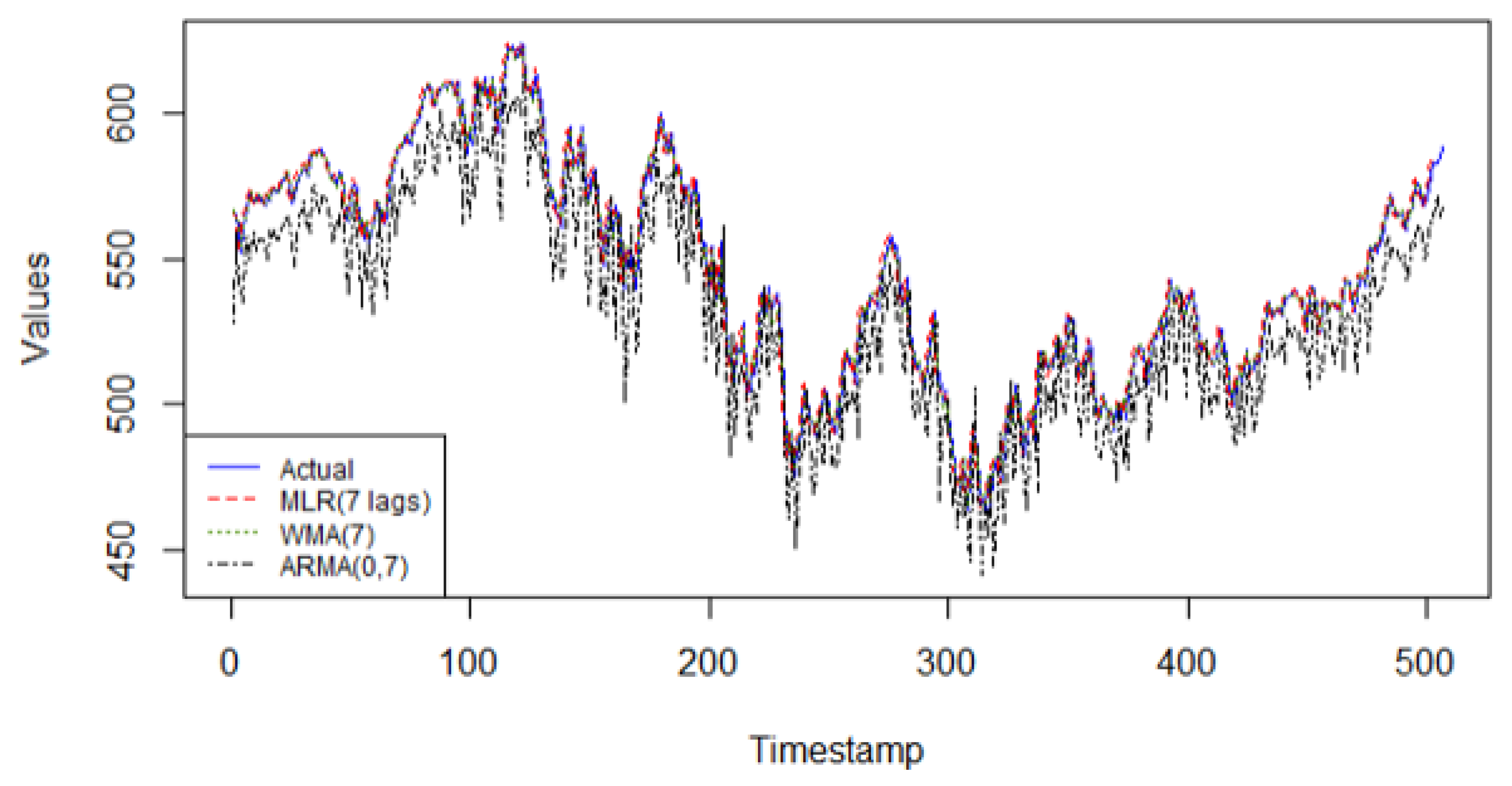
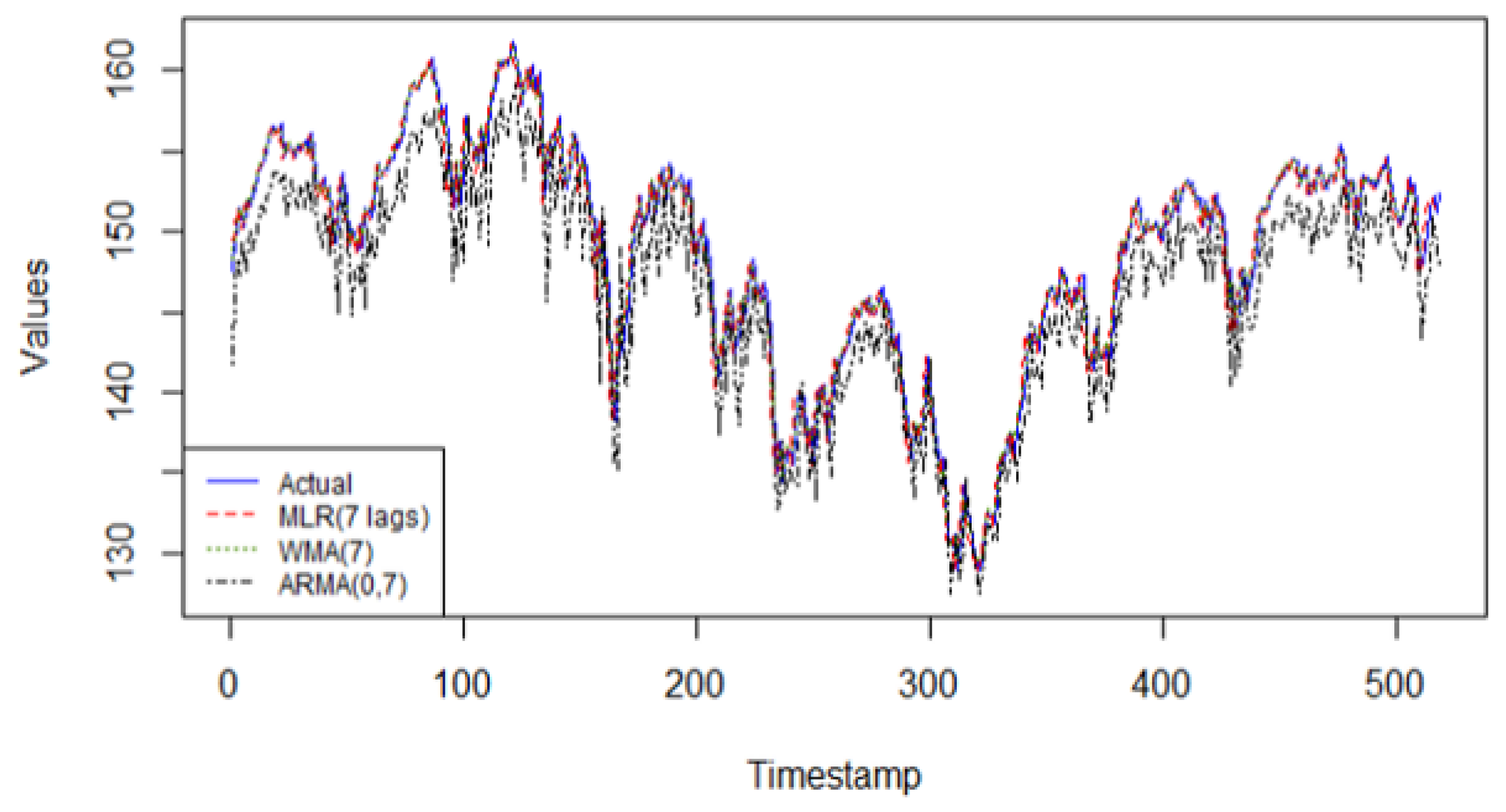
From Figure 1, the MLR(7) model provides the best linear fit for this time series. Historical data are very important to improve future predictions for this series. The MLR model offers different weights to each of the 7 lagged values, making this model adaptable to the data it is fitting. Additionally, the model provides an easy to interpret framework, making it easy to understand and to add on more predictors, external or not. It is also to be noted that generally, ARMA(0, q) models do not fit well to more complex nonlinear patterns. As for the weighted moving average model, WMA(7), its lack of “data-driven” characteristics explains its weak predictive performance on this series.

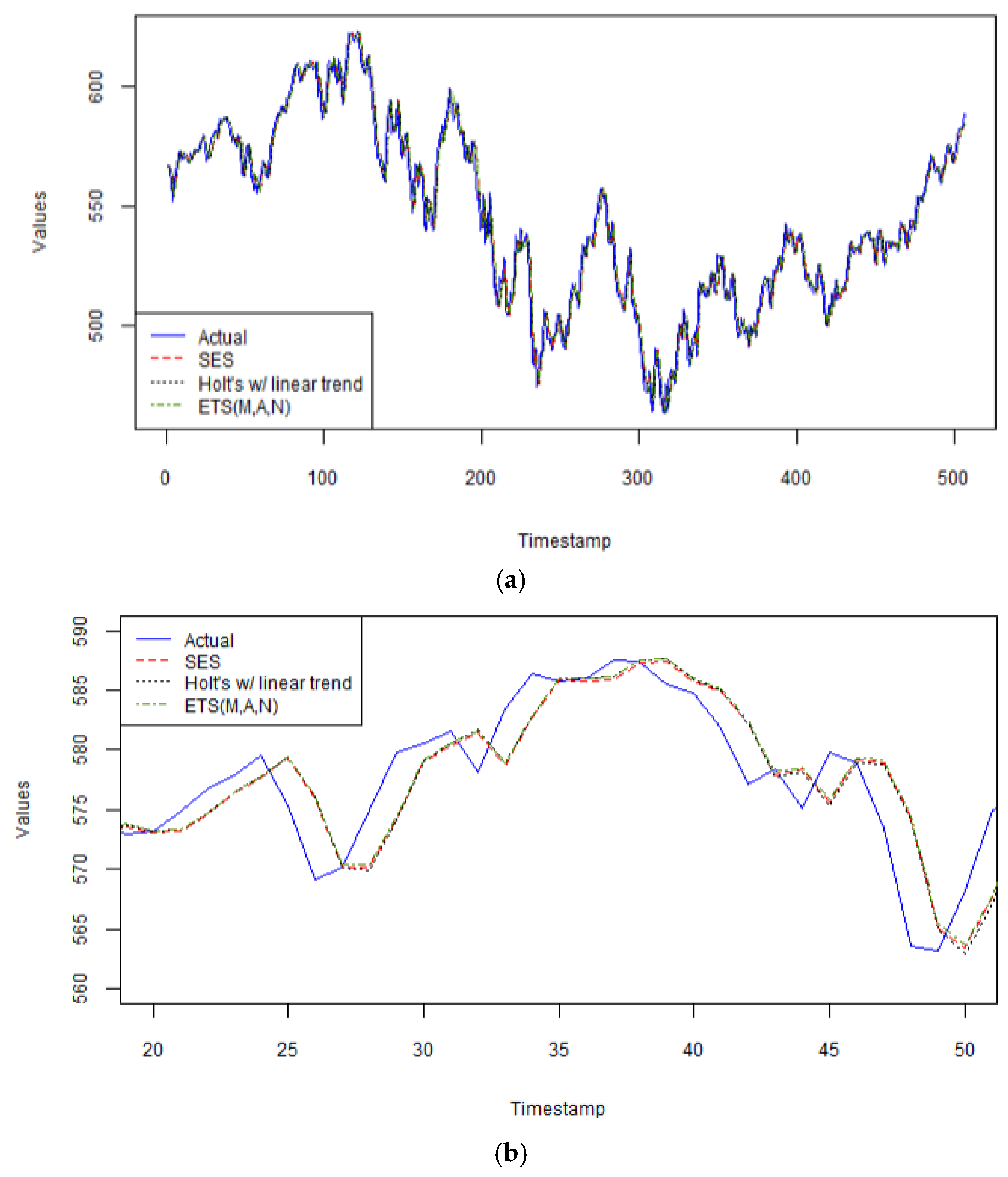
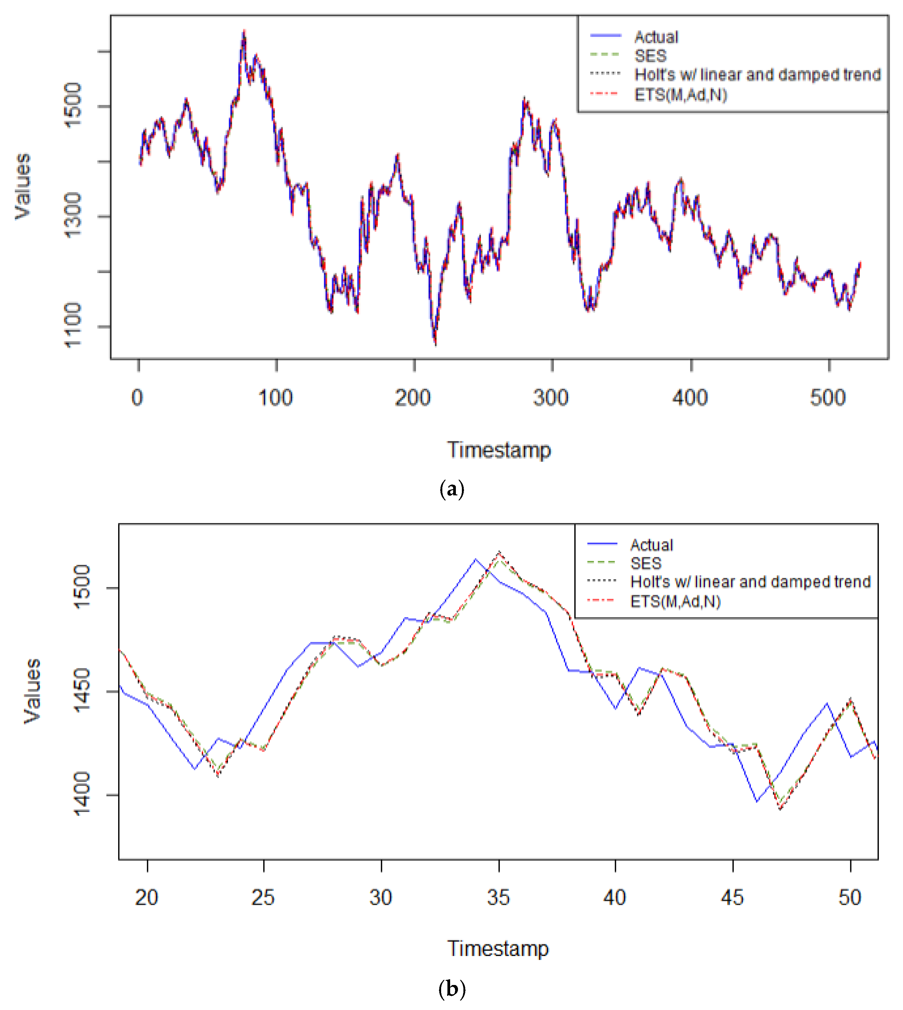
As seen in Figure 2a, all three exponential smoothing models perform exceptionally well on this series, with the simplest one, the SES model, having the best performance, as seen more up close in Figure 2b, between arbitrary time periods 20 and 50 in the validation dataset. Including past values with exponentially decreasing weights on each past value is the best way to obtain the most accurate forecast results for this series. A smoothing parameter, α = 0.91 means that this model is very responsive to the most recent observation, which implies that this model is also highly sensitive to random noise. Furthermore, identifying a long-term trend is statistically dubious with this series. Indeed, the data present high volatility, and therefore, a simple model with few parameters, such as SES, offers more robustness and generalizability to the noise contained in this series than Holt’s method with linear trend (α = 0.8488, β = 0.0001), or the automated selected model with an ETS configuration of multiplicative error with additive trend (α = 0.8726, β = 0.0001). Holt’s method requires additional parameters for trend, and damped trend, requiring estimation. If Holt’s methods (2) yield slightly higher performance metrics than the SES method, then the estimated parameters in the former method are not adding value to the forecasts and tend to overfit the data.

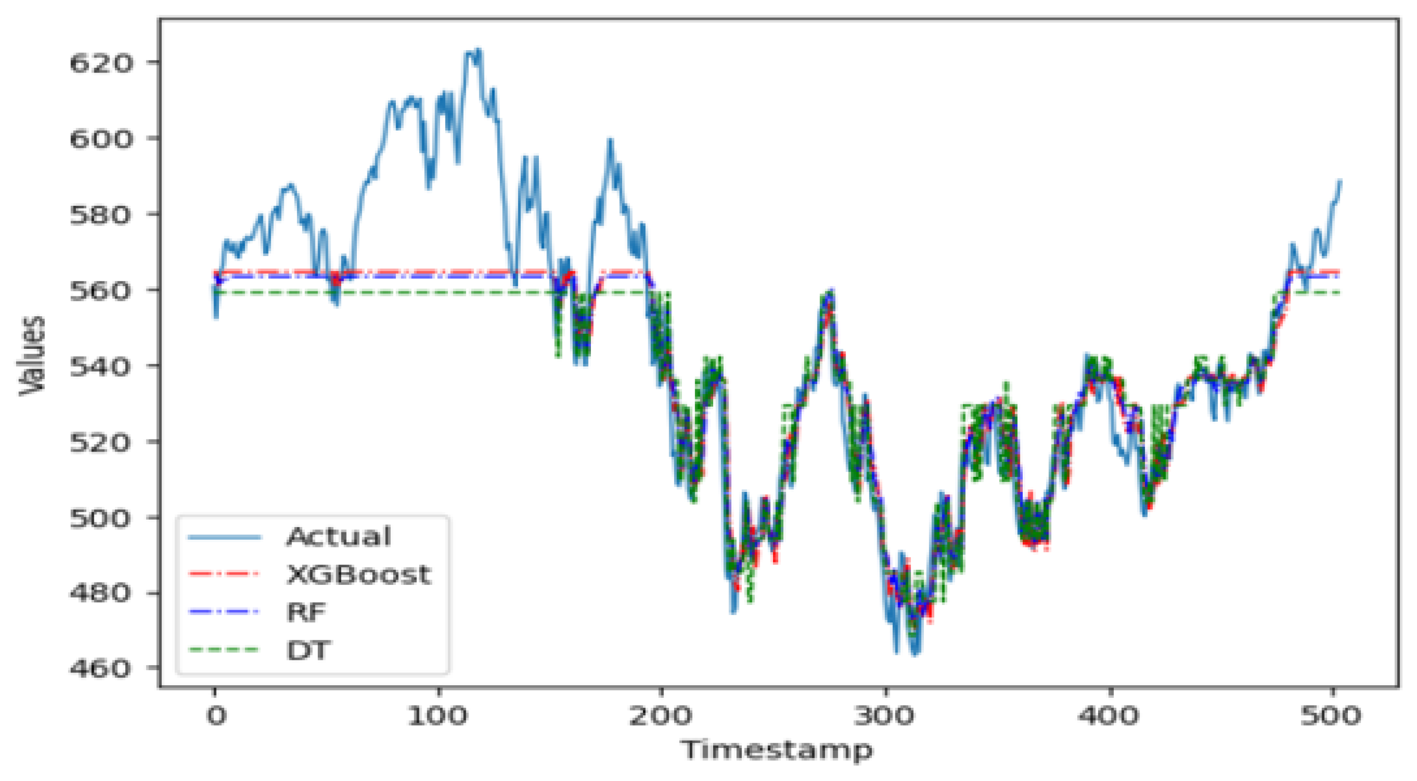
The plot in Figure 3 shows that the three machine learning algorithms only start to provide a good fit for the validation data after approximately first 200 time periods. This can be attributed to the fact that the performance of machine learning algorithms is highly sensitive to the selection of its hyperparameter values. A manual fine-tuning to find optimal values can prove to be tedious and time-consuming, adding a layer of difficulty and challenge to the prediction task. Therefore, an automatic optimization mechanism of the hyperparameters is essential to obtain optimal values in a faster time and without any manual effort. Indeed, the complexity of hyperparameter fine-tuning arises from the imposition of large, multidimensional search spaces in pursuit of optimal results, which is computationally expensive in terms of execution time [41]. In this regard, the implementation of a random search mechanism using the Bayesian search algorithm is worth considering for future work, with the goal to fine-tune the hyperparameters of these machine learning models. This search mechanism would be more effective for the type of time series examined in this study [42,43].

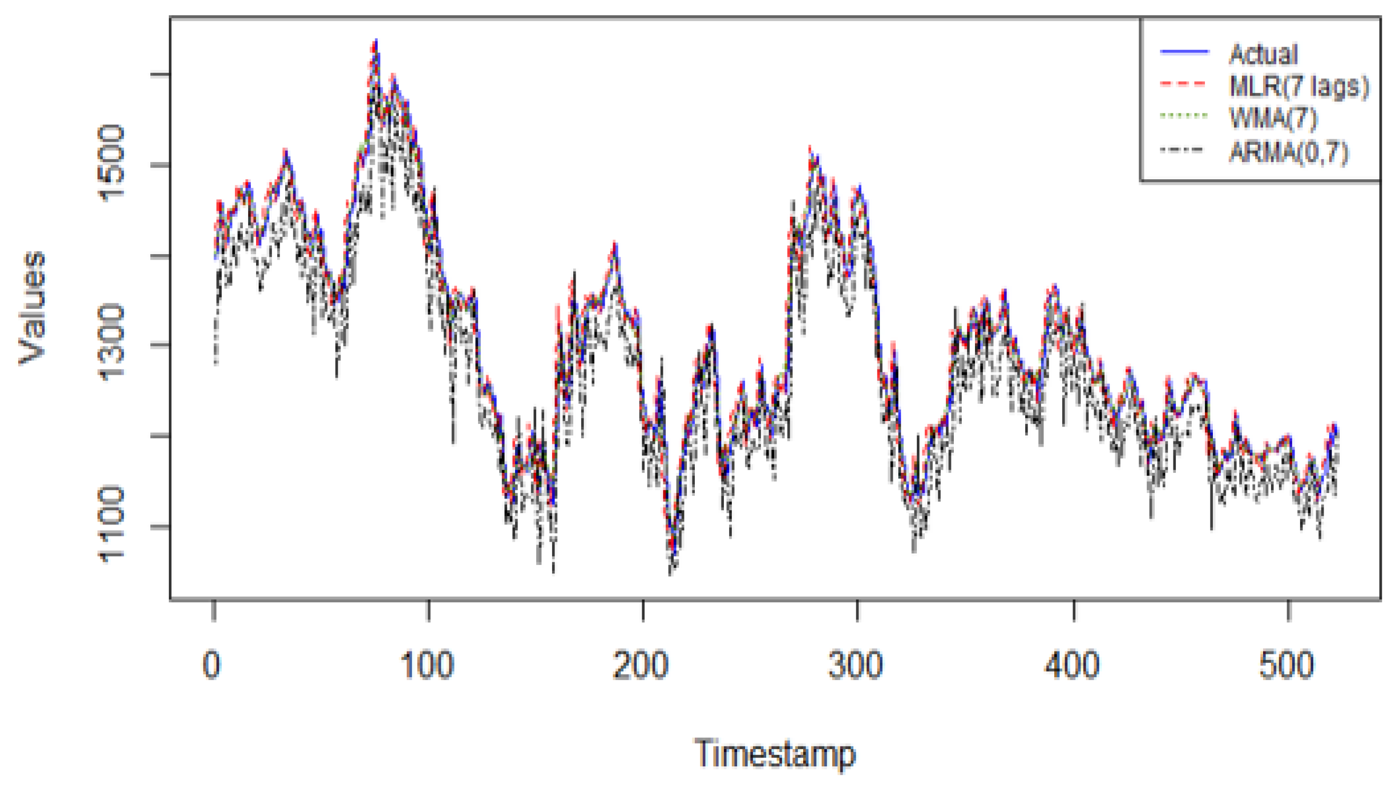
Figure 4 shows that in this time series, the linear regression model with 7 lagged values excels in its predictive capabilities for the single step forecasting task. The performance metrics on the validation data indicate high accuracy measures compared to the other linear models and even compared to all other models studied in this research. The WMA(k) and the ARMA(0, q) models fail to capture the patterns in this series due to the inability to capture nonlinear patterns in the latter method, and the lack of adaptability found in the former method.

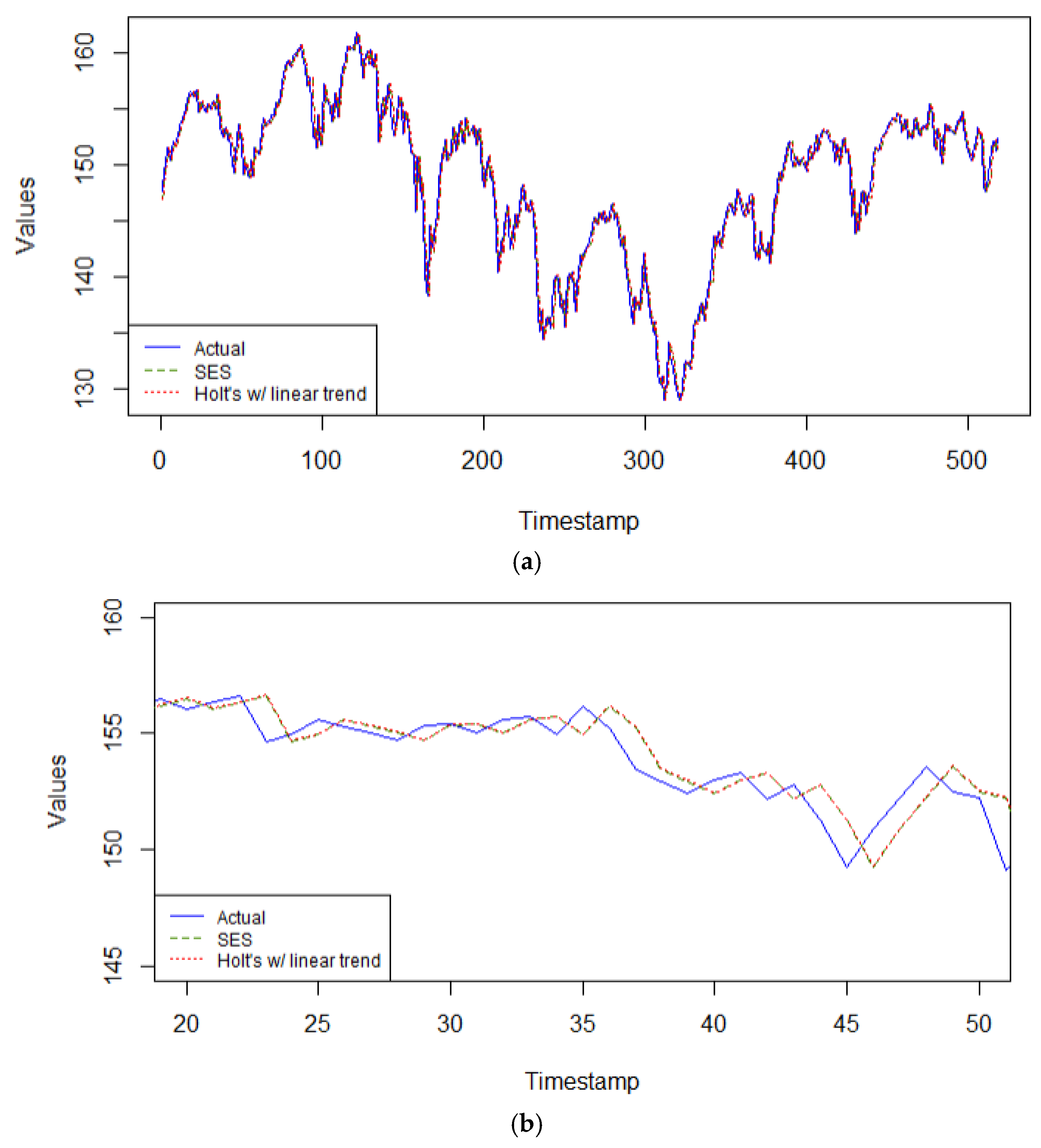
Again, the family of exponential smoothing models produce the highest accuracy predictions on this time series, as seen in Figure 5a, and further magnified in Figure 5b, capturing the arbitrary time periods of 20 to 50 of the validation data. This is due to their inherit characteristics of being able to handle nonlinear data and non-stationary too for short term forecasts. Of this set of models, Holt’s method with multiplicative error and damped linear trend, selected by the automated least AIC in Rstudio v. 4.3.2 with parameter values α = 0.9999, β = 0.078, φ = 0.80, is the best performing model on the validation data. The other two models are close in accuracy performance, with the SES model having a smoothing parameter, α = 0.9999, and the Holt’s linear model with parameters α = 0.9999, β = 0.1285, φ = 0.80.

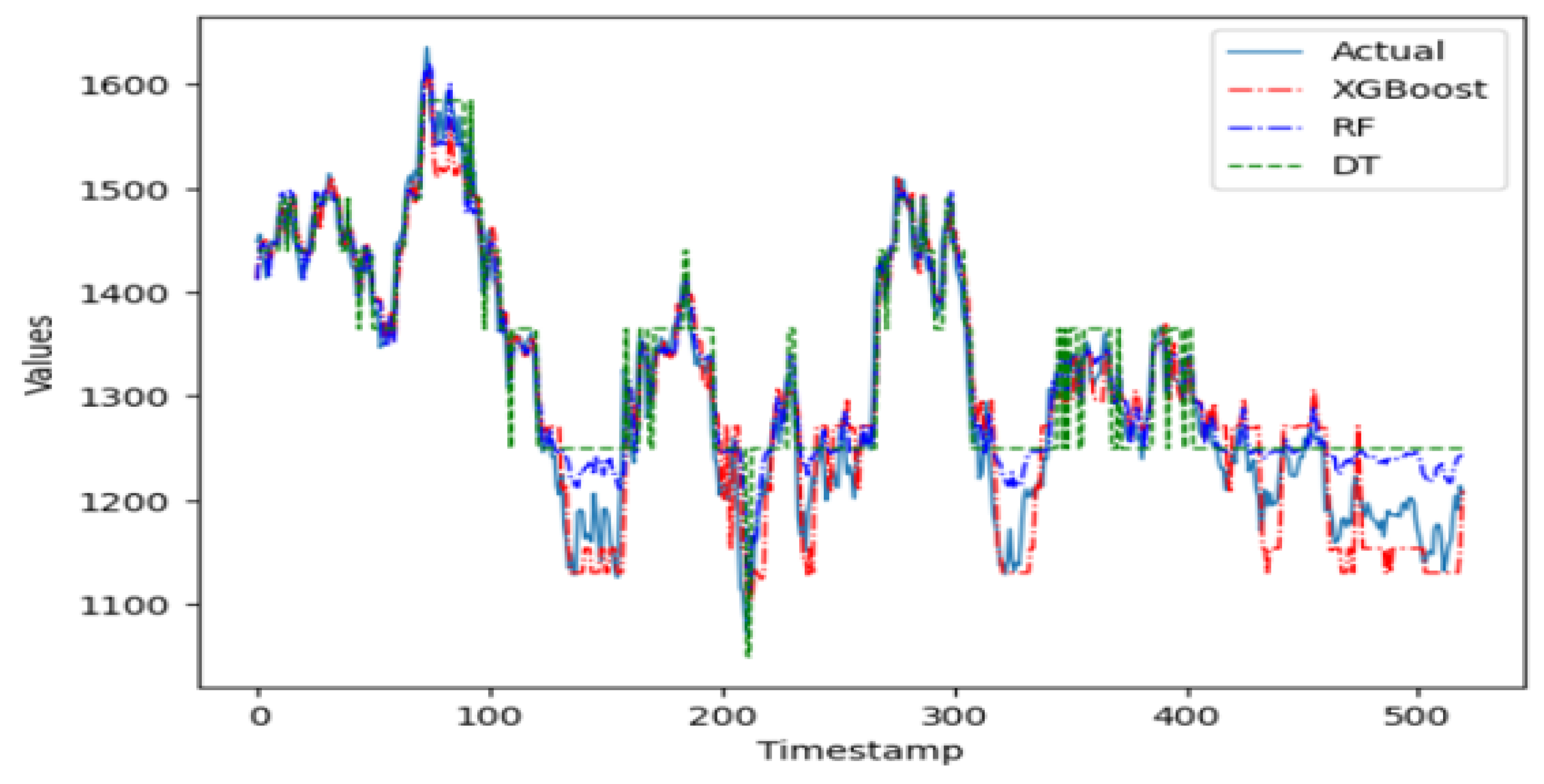
In the group of machine learning algorithms, it is evident in Figure 6 that the XGBoost predictor does not perform well on this time series. Being a complex model that is sensitive to parameter tuning, the XGBoost predictor does not fit this time series well when working with an ensemble of pruned trees. The random forest ensemble predictor, however, is a simpler model robust to parameter tuning and apt to perform better on this series when working with pruned trees. Indeed, this ensemble model performs better than the single regression tree. The random forest model is parametrized with 100 trees, with at most 10 levels per tree and no more than 50 leaf nodes per tree.

In the Sustainability European Index series, the linear regression model with 7 lagged values as predictors achieves the highest predictive accuracy when compared to the other linear models, as observed in Figure 7. The WMA(7) and ARMA(0, 7) models do not have the characteristics needed to fit the data adequately.

With this same series, the ETS model selected by the automated minimum AIC coincides with the simple exponential smoothing model (i.e., ETS(A,N,N)), with smoothing parameter α = 0.9999. Therefore, only two models are competing in the category of exponential smoothing models: the SES model = ETS(A,N,N) model, and Holt’s linear trend model with α = 0.9999, β = 0.0001, in Figure 8a,b. In both models, practically all the predictive power depends on the most recent observation, echoing a random walk model. It is responsive to the latest changes in the data. Since this series does not have a clear trend nor seasonal patterns, these two exponential smoothing models are very relevant for this single step forecasting task.

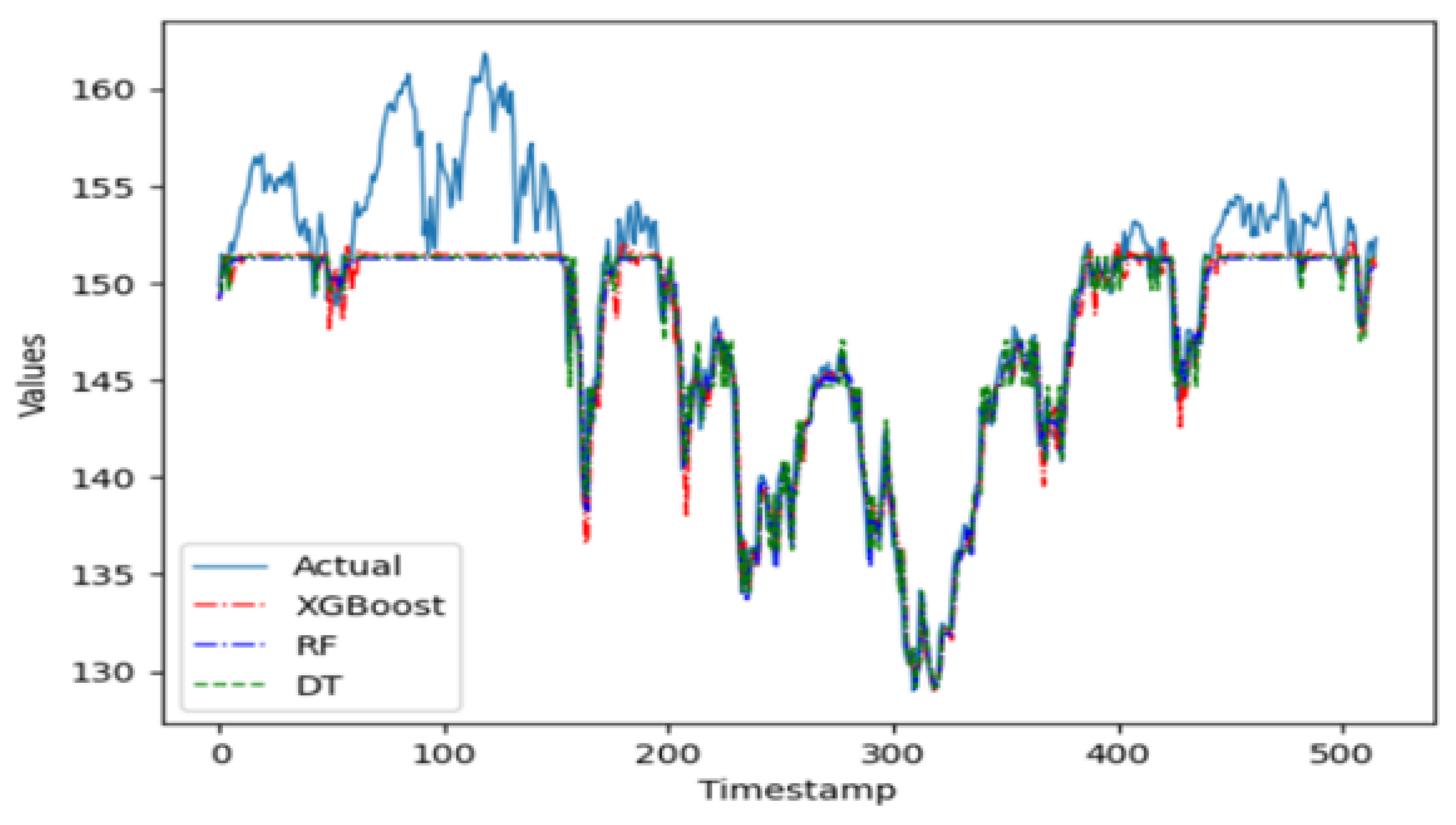
Figure 9 shows how all three machine learning algorithms start to provide a good fit for the validation data after the first approximately 150 time periods. This can be attributed to the fact that these types of algorithms need a substantial number of time periods before for optimal tuning to guarantee the most accurate and robust forecasts. Overall, the three methods perform very closely alike on the validation data. The evaluation metrics indicate, however, that the more complex ensemble model of XGBoost performs slightly better than the other machine learning methods, consisting of 100 shallow trees of depth not exceeding 5 levels per tree, and a learning rate = 0.1.

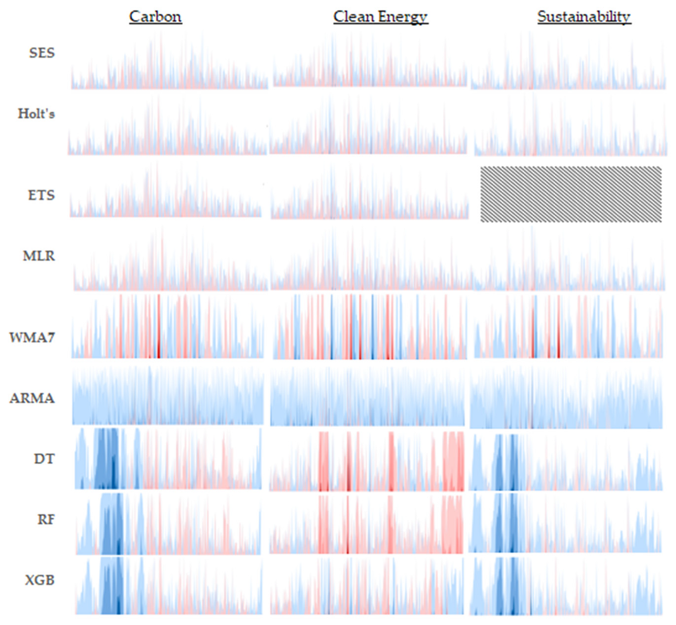
To enhance the interpretability of each predictive model’s performance, the absolute difference in each predicted value relative to the observed value is tabulated at each time period and over the entire course of the validation timeframe. These differences are then plotted in a horizon chart, as seen in Figure 10. Much like a heat map, color bands are used to show the extent to which a prediction deviates from its corresponding observed value at a given time period. Lighter color bands indicate lower deviations, while darker shades highlight significant discrepancies, allowing for a quick assessment of a model’s predictive accuracy over time. In this study, the blue-toned bands represent positive relative differences, and the pink-to-red-toned ones indicate negative relative differences. Arranging the horizon charts for all models in a grid, this format provides a visually intuitive and space-efficient means to analyze deviations across the entire validation timeframe per model and to compare model performance effectively per time series dataset. The figure’s content also exhibits the relative error distributions per the three families of models across the three distinct time series. Observing that exponential-based models consistently exhibit smaller relative errors across various validation datasets suggests a higher level of reliability and robustness. Consequently, these models are particularly advantageous in applications where precision is critical and maintaining low error rates is essential.

The performance measures of each model evaluated per time series are summarized in

Table 2. Carbon Efficient Index single step forecast accuracy results.

Model	MAE	MAPE (%)	RMSE	CPT (s.)
MLR(7 lags) w/int	5.2491	0.9777	6.7842	0.0159
WMA(7)	10.7012	1.9917	13.7353	2.1021
ARMA(0, 7) + Mean	14.7850	2.7034	17.1657	0.7776
SES	5.0859	0.9462	6.6134	0.0155
Holt’s method	5.0920	0.9475	6.6302	0.0304
Holt’s method w/multiplicative error and additive trend (ETS(M,A,N))	5.1245	0.9475	6.6432	0.1212
Regression Trees	14.7944	2.6131	20.5960	2.4498
Random Forest	12.5654	2.2147	18.2499	78.6277
XGBoost	11.9333	2.1005	17.4958	10.6253

,

Table 3. Global Clean Energy Index single step forecast accuracy results.

Model	MAE	MAPE (%)	RMSE	CPT (s)
MLR(7 lags) w/int	16.4735	1.2680	21.7911	0.0083
WMA(7)	39.8863	3.0749	51.6478	2.2254
ARMA(0, 7) + Mean	41.1300	3.1345	48.9320	0.4366
SES	16.5046	1.2705	21.9194	0.01430
Holt’s method w/damped trend	16.4873	1.2691	21.9060	0.0670
Holt’s method w/multiplicative error and damped trend (ETS(M,Ad,N))	16.4721	1.2680	21.8726	0.1291
Regression Trees	35.9727	2.8975	47.3698	0.7021
Random Forest	29.8887	2.3916	38.0445	83.4868
XGBoost	27.6875	2.1696	35.1229	12.2995

and

Table 4. Dow Jones Sustainability Europe Index single-step forecast accuracy results.

Model	MAE	MAPE (%)	RMSE	CPT (s)
MLR(7 lags) w/int	1.0157	0.6893	1.3715	0.0091
WMA(7)	2.2444	1.5325	2.9261	2.2128
ARMA(0, 7) + Mean	2.5318	1.6894	2.9366	0.6152
SES	1.0070	0.6841	1.3689	0.0124
Holt’s method w/linear trend	1.0057	0.6833	1.3694	0.0657
Regression Trees	2.2046	1.4500	3.0887	0.6497
Random Forest	2.3270	1.5283	3.2760	79.9538
XGBoost	2.690	1.4910	3.1750	12.9288

shown below. For instance, Table 2 shows that the lowest forecasting error for the carbon-efficient market is obtained by SES. The ARMA and regression trees yielded the highest forecasting errors. Their performances are similar, while ensemble trees (random forest and XGBoost) outperformed the regression trees. For the global clean energy market, Table 3 shows that the lowest forecasting error is obtained by Holt’s method with multiplicative error and damped trend (ETS(M,Ad,N)). The ARMA yielded the highest forecasting errors. The ensemble trees, namely the random forest, outperformed the regression trees. Finally, for the Dow Jones sustainability index, both SES and Holt’s method with a linear trend yielded the lowest forecasting error (Table 4). In addition, their performances are similar. Meanwhile, regression trees yielded the highest forecasting error. The ensemble XGBoost outperformed the standard regression trees. In all three index time series, the SES model achieved the lowest RMSE and CPT values, or was a very close contender, particularly with the Clean Energy index time series. This underscores the efficacy of exponential smoothing models as reliable real-time predictors for investors who need to react swiftly to volatile price changes and emerging market trends.

When working with original data that have not been subject to any preprocessing, it is clear from the findings in this study that the classical time series models are the most accurate methods for one-step ahead forecasts. The computational complexity associated with these models on highly complex data patterns is low compared to the linear models and the machine learning ones. The simple exponential smoothing model is especially efficient for short-term forecasting tasks.

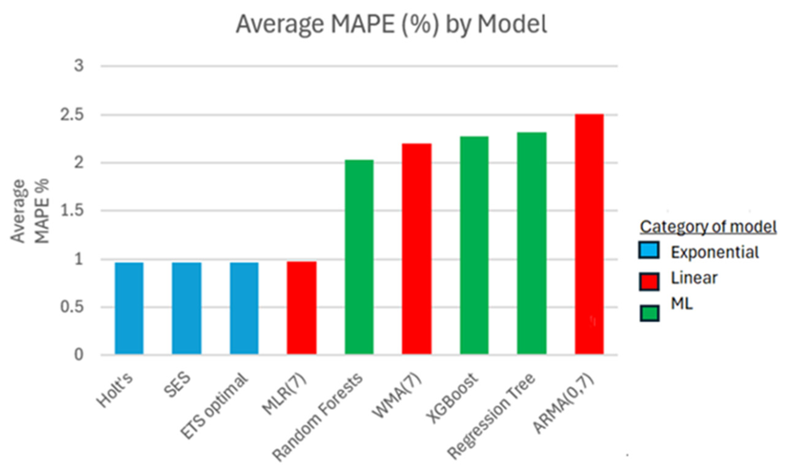
In Figure 11, the overall performance of each model is represented by taking the average of the MAPE value (in %) per model and across all three series. Widely used in the financial industry due to its easy to interpret results while emphasizing the magnitude of an error incurred between the actual and forecasted value, relative to the actual value, the MAPE is a good measure to use for this assessment [44,45]. It warrants a reliable scale-free comparison of the forecast performances across all three time series and for all models. As expected, all three exponential smoothing models have the best MAPE measure accuracy for one-step ahead forecasts. The linear models perform somewhat better than the machine learning ones. Indeed, the MLR(7) model leads in its linear category, while the random forests have the best accuracy results in its machine learning category. More formal comparisons through statistical tests cannot be performed as there are too few groups of models per time series to compare against. Hence, the findings from this study do not provide enough evidence to support statistically significant generalizations. Nevertheless, these findings highlight the potential of traditional exponential-based models and their capabilities in predictive analysis.

5. Discussion and Conclusions

As the world shifts from fossil fuels to low-carbon energy sources, green market equities are becoming increasingly popular among investors and policymakers. It follows that there is a growing interest in having highly accurate forecasts available for important decision-making endeavors. An overview of the literature on financial green market prediction revealed that there had been many studies using different approaches, including statistical methods and machine learning approaches. However, this is the first study (to the best of our knowledge) that has been used to conduct a comparison between various statistical models and ensemble-based machine learning systems. Furthermore, the comparison between different standard ensemble learning models in the context of green finance is missing, which needs further investigation. Consequently, this study empirically evaluates the added value of some machine learning methods by applying them to three green market time series and comparing their short-term forecast accuracies to those obtained from the more traditional time series models. Finally, the question of the robustness of single-step forecasts across the nine different models evaluated in this study is addressed.

Evidence from this study shows that the simple and versatile exponential smoothing models produce the most accurate forecasting results on some of the more complex time series available, regardless of the characteristics of the data. Meanwhile, ensemble methods analyzed by bootstrapping with XGBoost, or bagging with random forests, perform better than a single regression tree, yet they are outperformed by the exponential models. This is demonstrated with the carbon efficiency index, where the highest accuracy was obtained with the SES model on all performance measures. The clean energy index series rendered the best forecast accuracy results that were shared between a member of the exponential family of models, the Holt’s method with a configuration of ETS(M,Ad,N), and a member of the linear models, the multiple regression model with 7 lags. The sustainability Europe index had its highest accuracies found within the exponential family of models, between the SES model and Holt’s method with a linear trend. With its proven ability to dynamically adjust to shifting trends and seasonality patterns, the exponential smoothing models can capture both short-term fluctuations and long-term patterns. Secondly, the recursive weighted averaging scheme that the exponential smoothing models apply to the data for each new observation generates a nonlinear algorithm characterized by exponentially decaying weights for less recent observations. Indeed, this family of models has the remarkable ability to intricately decompose a time series into the different patterns of trend, seasonality, and error components without relying on any data preprocessing method, but rather simply by recursively updating parameter estimates for each accounted component. Hence, the exponential smoothing method is flexible and responds quickly to abrupt changes in the data by virtue of its smoothing parameters. Lastly, the exponential smoothing is simple and easy to implement.

Conversely, the accuracy metrics based upon the minimization of some loss function involve more computational intricacies for the ML methods driven by nonlinear algorithms to reach minimization than for the traditional models [46]. As seen in the graphs of the regression-trees based ML models in this study, it takes many time periods before these models start to provide a good fit to the data. The underperformance of the decision trees can also be attributed to inadequate optimization techniques implemented in the three respective ML algorithms to fine-tune their parameters. Indeed, their effectiveness relies on the choice of value of its parameters. Ensuring the inclusion of an adequate optimization technique to find optimal parameter values to build the regression trees will improve the learning and data-fitting steps and reduce the forecasting error.

Meanwhile, this study confirms that there is added value in using an ensemble approach by combining many decision trees to yield higher accuracy measures than those found from a single tree model. This result is true for all three green markets examined, highlighting the importance of combining multiple models to reduce noise and enhance predictive accuracy. The XGBoost model performs better than the random forest model in two of the three green finance markets. This is likely because XGBoost uses an iterative and sequential approach by fitting consecutive decision trees and always working to reduce the errors incurred by the previous trees, allowing for any complex interactions between features, in this case the seven consecutive lags, to be included in the model, unlike in the random forest model. The XGBoost model also benefits from a regularization term to prevent overfitting and give a more robust model than the random forest one.

In closing, this study finds that the traditional models of exponential smoothing successfully achieve the highest accuracies on single-step forecasts for the original time series of green finance markets. The implications are that these univariate models inherently offer a conveniently simple and quick solution for single-step predictions when the original time series follows a right-skewed distribution. The forecasts obtained will improve short-term decision-making for investors and traders, ultimately generating significant profits. Since simpler models are computationally more cost-efficient than complex ones due to their ease of implementation and interpretation, this gives investors an added incentive to adopt data-driven decision-making, while traders will be more inclined to test multiple market scenarios for optimal results without too much time delay due to the low time efficiency and simplicity that the exponential-based models encompass. Albeit regression tree-based models are worthwhile for managers and investors to consider using in their decision-making process as their algorithms are based on if-then rules, offering a more all-encompassing view on forecasts obtained. In this regard, they are intuitive and easy to understand and interpret. With an appropriate optimization method in place to fine-tune their key parameters, the regression-tree-based models should provide improved forecast accuracy.

For future research, one could incorporate external factors into the models, thereby transitioning to multivariate approaches. Additionally, applying advanced machine learning models and exploring various optimization techniques to fine-tune their parameters may yield significant improvements. Another avenue for future investigation involves including other green finance markets to enrich the study and facilitate more comprehensive comparisons. Finally, given the volatility and unpredictable nature of these green market time series, future work may explore the results obtained after the implementation of a decomposition method on the data to improve the forecasting task.