Short-Term Load Forecasting in Distribution Substation Using Autoencoder and Radial Basis Function Neural Networks: A Case Study in India

Abstract

Electric load forecasting is an essential task for Distribution System Operators in order to achieve proper planning, high integration of small-scale production from renewable energy sources, and to define effective marketing strategies. In this framework, machine learning and data dimensionality reduction techniques can be useful for building more efficient tools for electrical energy load prediction. In this paper, a machine learning model based on a combination of a radial basis function neural network and an autoencoder is used to forecast the electric load on a 33/11 kV substation located in Godishala, Warangal, India. One year of historical data on an electrical substation and weather are considered to assess the effectiveness of the proposed model. The impact of weather, day, and season status on load forecasting is also considered. The input dataset dimensionality is reduced using autoencoder to build a light-weight machine learning model to be deployed on edge devices. The proposed methodology is supported by a comparison with the state of the art based on extensive numerical simulations.

1. Introduction

Utility companies must estimate electrical power consumption in order to reduce operating and maintenance costs, manage demand and supply, increase dependability, properly plan for future investments, and engage in efficient energy trading [1,2,3]. Based on the forecasting time, electrical load forecasting may be broadly classified into four primary categories: extremely short-term and short-term [4,5], medium-term, and long-term load forecasting [6]. Depending on the time horizon, load forecasting can be used for a variety of purposes, including optimal operations, grid stability, demand-side management (DSM), or long-term strategic planning [7].

One of the more difficult problems in a deregulated power system is anticipating short-term active power load. Load consumption patterns are more commonly adjusted as a result of weather, cultural events, and people’s social routines, according to [8]. The active power load in low-voltage distribution systems is very unpredictable, particularly in India, because the majority of customers are residential and commercial customers who are heavily impacted by the considerations stated above. As a result, accurate forecasting of active power load is a crucial responsibility for distribution system operators for proper distribution network operational planning and energy trading. As shown in Table 1, much work has been carried out on the demand-side forecasting problem for accurate prediction using artificial intelligence (AI) techniques.

Table 1. Literature survey on short-term load forecasting.

Reference	Features
	A	B	C	D	E	F	G
[9]	√	√	-	-	-	-	LGBM, XGB, MLP
[10]	√	-	-	-	-	-	CNN
[11]	√	√	√	-	-	-	DNN
[12]	√	-	-	-	-	-	MCM
[13]	√	-	-	-	-	-	SVM, RF, LSTM
[14]	√	-	-	√	-	-	MLPNN, GDBT
[15]	√		-	-	-	CNN	GRU, LSTM
[16]	√		-	-	-	CNN	LSTM
[17]	√		-	-	-	-	Linear Regression, LSTM
[18]	√	√	√	-	-	CNN	LSTM
[19]	√	√	-	√	√	-	CNN, DRN
[20]	√	√	-	-	-	-	Probabilistic Model
[21]	√	-	-	-	-	-	Linear Regression
[22]	√	-	-	-	-	-	IPSO, LSTM
[23]	√	-	-	-	-	-	GRU, Diffusion Model
[24]	√	√	√	√	√	-	Regression Tree
A: Historical load data			B: Historical temperature data
C: Historical humidity data				D: Day type		E: Season
F: Dimensionality reduction				G: AI model

All the instances of the literature mentioned in Table 1 have made a significant contribution to dealing with short-term electric power load forecasting issues. A new strategy is proposed in this study to increase forecasting accuracy and to design a light-weight model for active power load forecasting applied to a 33/11 kV substation by employing autoencoder (AE) for dimensionality reduction and a Radial Basis Function Neural Network (RBFNN) for load forecasting.

The major contributions and constraints considered in this paper can be summarized as follows:

• Electric power is forecasted one hour ahead by considering the status of the day, i.e., weekend/weekday. As the 33/11 kV substation is located in Godishala, Warangal, where all offices and colleges are closed on Sunday, only Sunday is considered the weekend.
• Electric power is forecasted one hour ahead by considering the season. In India, there are three seasons, i.e., Winter (November–February), Summer (March–June), and Rainy (July–October).
• Electric power is forecasted one hour ahead by considering the weather condition in terms of temperature and humidity.
• Electric power is forecasted one hour ahead by considering the last four hours of load data, i.e., P(T-1), P(T-2), P(T-3), and P(T-4), and by considering the load of the last four days, i.e., P(T-24), P(T-48), P(T-72), and P(T-96).
• A new optimal autoencoder architecture is developed to reduce the dimensions of the dataset from 8664 × 12 to 8664 × 9.
• A new optimal RBFNN architecture is developed to forecast the load using the compressed data.

The remainder of the paper is organized as follows: Section 2 demonstrates methodology developed to forecast the load and to reduce the dimensions of the dataset; Section 3 presents simulation results; and in Section 4, some conclusions are drawn.

2. Materials and Methods

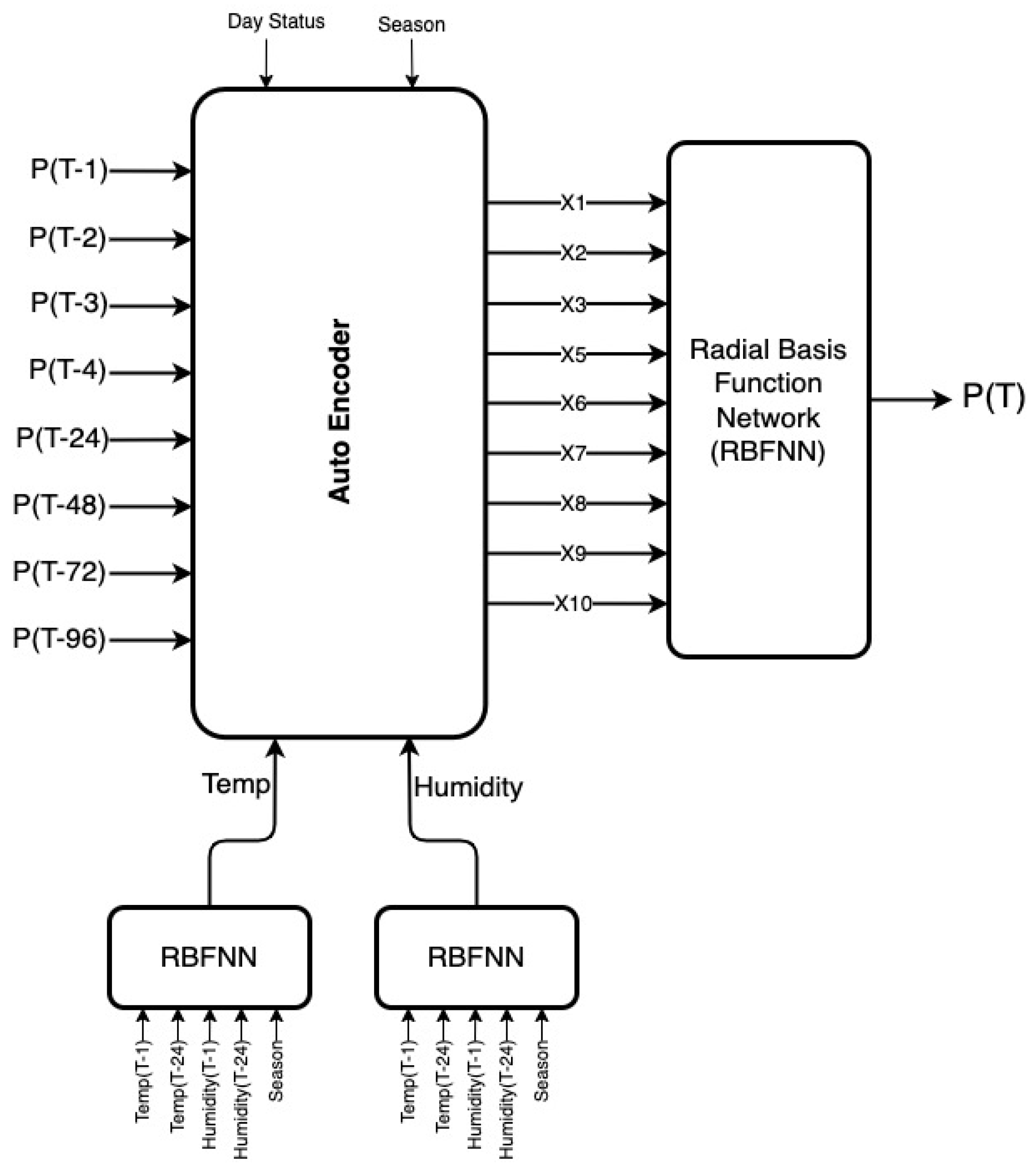
This section presents the detailed procedure we used for dimensionality reduction of the input dataset using AE for forecasting temperature, load, and humidity using RBFNN. The complete architecture for forecasting the load one hour ahead for effective trading an hour ahead in the energy market is shown in Figure 1. RBFNN and Autoencoder models are implemented in Google Colab with Python programming language having version 3.10.

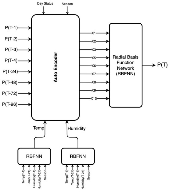
Figure 1. Short-term load forecasting architecture.

2.1. Active Power Load Dataset

The active power load dataset based on load data was collected from a 33/11 kV substation located in Godishala, Warangal, India, during the period from January 2021 to December 2021. In order to train and test the AE+RBFNN model, normalized data [25] were used and generated based on Equation (1). In this paper, forecasting the load depends upon previous load samples. Hence, the last four hours and last four days prior to the time of forecasting are considered. Also, load consumption varies based on season and day status (weekend/weekday) as well as temperature and humidity. In the region of Warangal, India, the summer temperature reaches 47 °C; in winter, it reaches 22 °C. These values indicate high impact load consumption. The data were collected during the period of January 2021 to December 2021, covering all weather conditions during the year and all temperature and humidity changes throughout the year. As our models were trained with these data, they are generalized across all types of load variations and seasonal variations

$$X_{N}orm={\displaystyle \frac{x-x_{min}}{x_{max}-x_{min}}}$$

(1)

2.2. Dimensionality Reduction Using Autoencoder (AE)

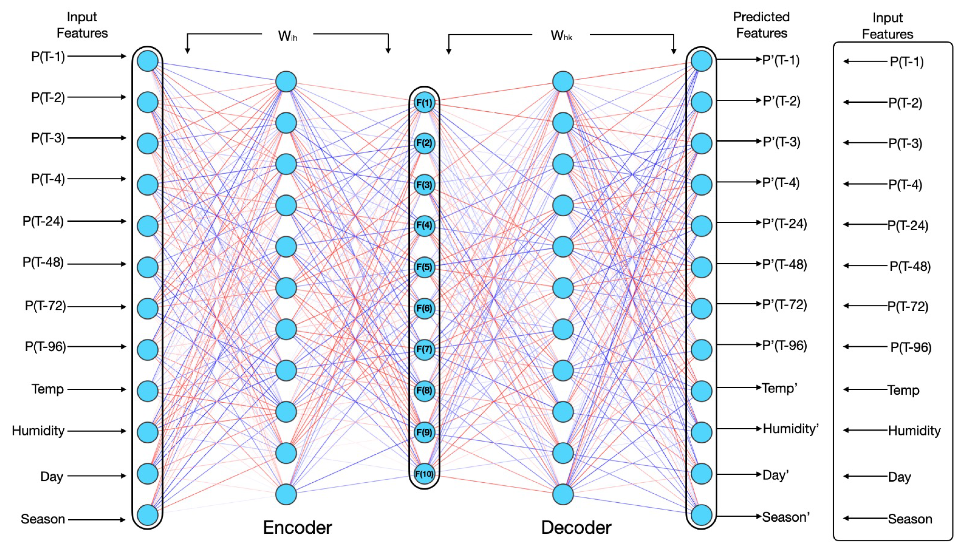
Autoencoder (AE) is a deep neural network that is used to reduce the dimensionality of input data and reconstruct the original data from the compressed representation. It has three parts: an encoder, latent space, and decoder. The encoder compresses the input data into a lower dimension in the latent space, whereas the decoder reconstructs the original data from lower-dimension compressed data available in the latent space [26]. In this paper, AE is used to convert higher-dimension original data of volume 8664 × 12 into lower-dimension compressed data of volume 8664 × 9. The complete architecture of AE with a ReLu activation function [27] in the latent space is shown in Figure 2.

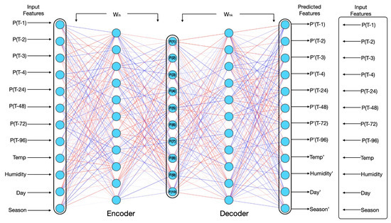
Figure 2. AE model architecture [28].

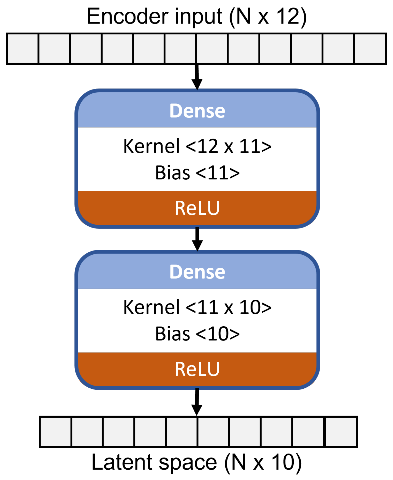
The architecture of the encoder part of the autoencoder, which provides lower-dimension data from higher-dimension original data, is shown in Figure 3. The data are compressed to 10 features from 12, while the fourth neuron in the latent space gives a zero value for all samples in the original dataset. Hence, the feature corresponding to the fourth neuron is removed, and the compressed data only have 9 features. The optimal AE model is identified by tuning hyperparameters like the number of hidden layers and neurons minimizing the following cost value:

$$C=0.5·\mathrm{NVL}+0.5·\mathrm{NVD}$$

(2)

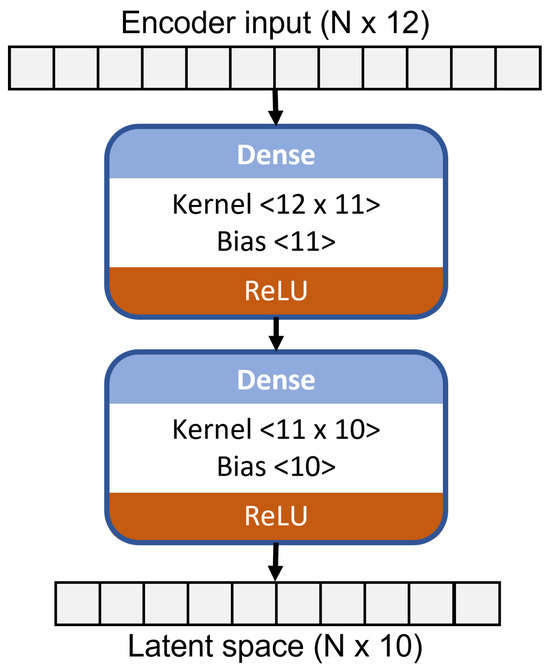
Figure 3. Encoder architecture.

The normalized validation loss (NVL) is defined by the following equation:

$$\mathrm{NVL}={\displaystyle \frac{\mathrm{VL}-{\mathrm{VL}}_{min}}{{\mathrm{VL}}_{max}-{\mathrm{VL}}_{min}}}$$

(3)

where ${\mathrm{VL}}_{min}$ and ${\mathrm{VL}}_{max}$ are the minimum and maximum validation loss among all observed architectures, and NVD is the normalized variance deviation of the compressed dataset from the original dataset.

The validation loss (VL) is computed by

$$\mathrm{VL}={\displaystyle \frac{1}{n_{sample}^{test}}}\sum _{sample=1}^{n_{sample}^{test}}{(d-o)}^2$$

(4)

where d and o represent the desired and actual outputs, respectively.

2.3. Radial Basis Function Neural Network (RBFNN)

RBFNN [29] is a machine learning model that can be used for both regression and classification problems. It has three layers: input, hidden, and output layers [30,31]. Unlike simple artificial neural networks, it uses both unsupervised and supervised learning strategies. Unsupervised learning, i.e., competitive learning [32] based on Euclidean distance (also called the k-means clustering algorithm) is used between the input and hidden layer, whereas supervised learning based on the back-propagation algorithm [33] is used between hidden and output layers. The Gaussian function [34,35] shown in Equation (5) is used as an activation function in the hidden layer and the linear activation function is used in the output layer. The optimal RBFNN architecture is identified based on validation loss shown in Equation (4) by tuning the hyperparameters of the RBFNN model as mentioned in [28]:

$$f\left(x\right)=e^{-{\displaystyle \frac{{(x-\mu )}^2}{2{\sigma }^2}}}$$

(5)

The advantages of RBFNN [36,37] for short-term laod forecasting are as indicated below:

• Electricity load patterns are highly nonlinear and depend on multiple factors (e.g., time, temperature, holidays). RBFNN uses Gaussian radial basis functions that allow it to approximate complex functions more effectively than simple linear models.
• Unlike deep learning models (e.g., LSTMs, CNNs), RBFNNs require fewer training epochs because they rely on localized activation functions.
• Traditional RBFNNs rely on raw input features, which may contain noise or irrelevant information.

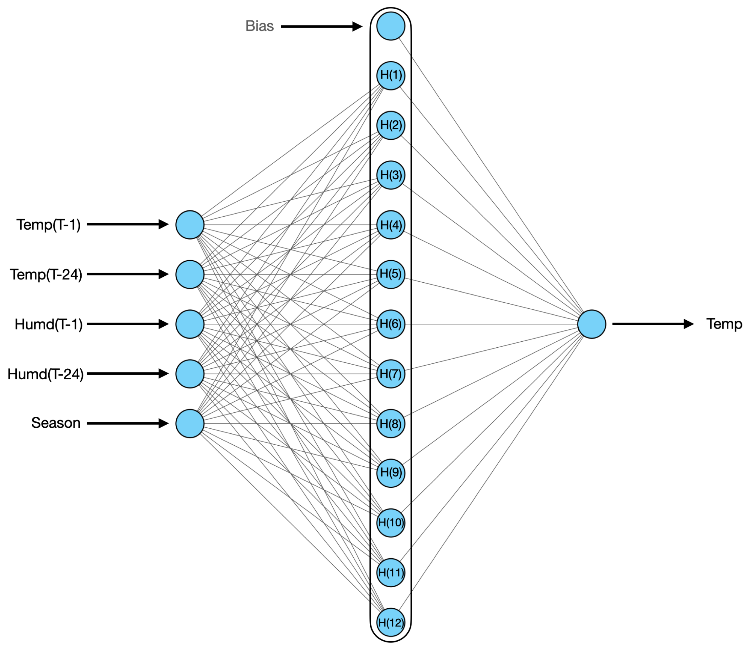
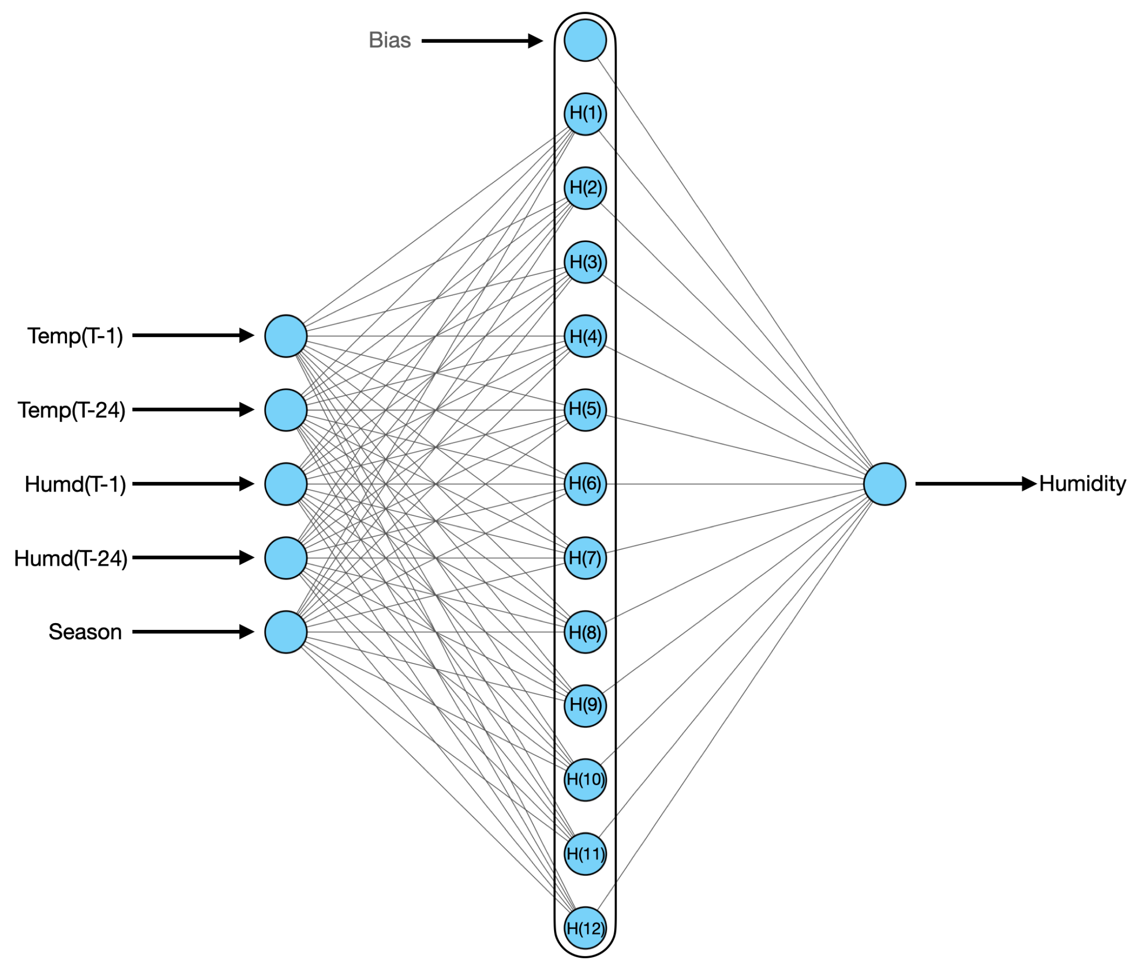
In this paper, the optimal architecture for RBFNN for temperature forecasting is shown in Figure 4; for humidity forecasting, it is shown in Figure 5. In this paper, RBFNN is used to forecast the load for a 33/11 kV substation based on features extracted by AE from original features. Temperature and humidity are the input features for AE and the result that comes from the output neuron of the RBFNN model is used for temperature and load forecasting, respectively, as shown in Figure 1. The optimal architecture of RBFNN for active power load forecasting is shown in Figure 6. The complete training algorithm for RBFNN is taken from [38].

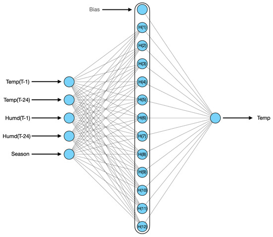
Figure 4. RBFNN is used to forecast temperature.

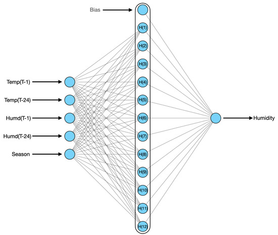
Figure 5. RBFNN is used to forecast humidity.

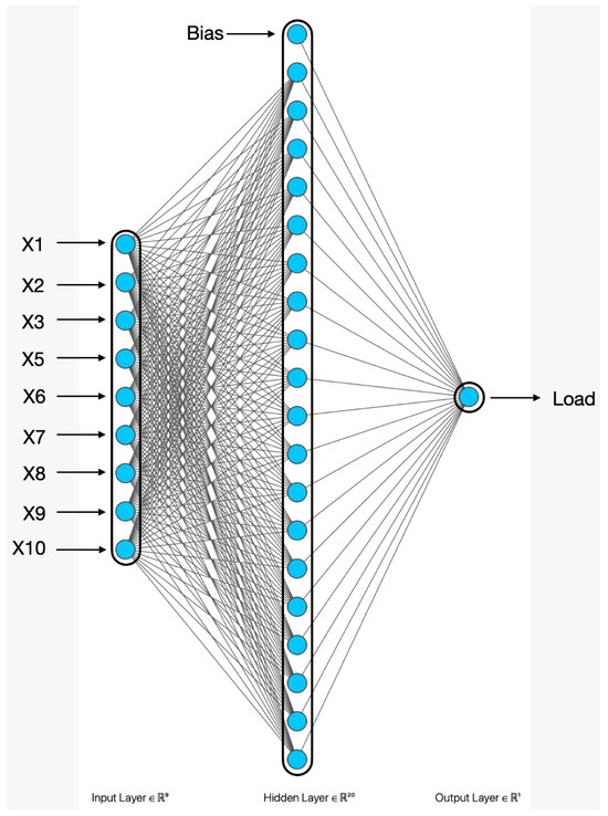
Figure 6. RBFNN is used to forecast active power load for 33/11 kV substation.

The combination of AE and RBFNN is useful to extract strengths from each model and to develop a better model [39,40]. The features of each individual model, AE and RBFNN, and the combined hybrid model are presented in Table 2.

Table 2. Features of RBFNN, AE, and AE + RBFNN models.

Feature	RBFNN	AE	RBFNN + AE
Handles Non-Linearity	√	√	√
Feature Extraction	×	√	√
Robust to Noise	×	√	√
Fast Training	√	√	√
Interpretable Model	√	×	√
Handling Missing Data	×	√	√

3. Results

To train and validate the RBFNN model for load forecasting and the AE for dimensionality reduction, historical load data were collected over the period 1 January to 31 December 2021 from a 33/11 kV substation in Godishala, Telangana State, India. This load dataset comprises 8760 total active power load samples (24 h × 365 days = 8760) rearranged into an 8664 × 12 matrix. This weather dataset was prepared based on the temperature and humidity data available at Weather Data-Online, available at https://www.wunderground.com/history/daily/in/kazipet/VOWA/date/2021-1-2 (accessed on 29 January 2022).The datasets were split 70%:30% for training and testing, respectively. Based on this ratio, the shape of the training and testing data for each model is shown in Table 3. The following procedure is used for the active power load forecasting.

Table 3. Training and testing data size.

Task	Dataset	Model	Data Shape
			Training	Testing
Data compression	Load Dataset	AE	5804 × 12	2860 × 12
Load forecasting	Compressed Data	RBFNN	5804 × 9	2860 × 9
Weather forecasting	Weather Data	RBFNN	5846 × 5	2890 × 5

• Dimensionality reduction using AE;
• Temperature forecasting using RBFNN;
• Humidity forecasting using RBFNN;
• Load forecasting using RBFNN;
• Web application development.

3.1. Data Insights

The stochastic features of the initial dataset that is used to forecast the load are shown in Table 4.

Table 4. Statistical information of original dataset.

Parameter	P(T-1)	P(T-2)	P(T-3)	P(T-4)	P(T-24)	P(T-48)
count	8664	8664	8664	8664	8664	8664
mean	2121	2121	2121	2121	2121	2121
std	1294	1294	1294	1294	1295	1295
min	458	456	456	456	456	432
25%	1063	1063	1063	1063	1063	1062
50%	1673	1673	1673	1673	1673	1673
75%	3001	3001	3001	3001	3005	3006
max	6306	6306	6306	6306	6306	6306
Parameter	P(T-72)	P(T-96)	DAY	SEASON	TEMP	HUMIDITY
count	8664	8664	8664	8664	8664	8664
mean	2120	2120	0	1	81	68
std	1295	1295	0	1	9	21
min	432	412	0	0	50	14
25%	1061	1061	0	0	77	52
50%	1673	1673	0	1	81	72
75%	3006	3007	0	2	86	87
max	6306	6306	1	2	108	102

3.2. Optimal AE for Dimensionality Reduction

In order to identify the optimal AE model, the AE model was trained and validated with various numbers of neurons in the hidden layer and various batch sizes. The mean square errors on the training and testing data are reported in Table 5.

Table 5. Error metric during AE training.

Latent Space	Mean Square Error
	BS: 8		BS: 16
	Training	Validation	Training	Validation
11	0.0180	0.0198	0.0091	0.0090
10	0.0117	0.0109	0.0082	0.0077
9	0.0116	0.0125	0.0125	0.0120
8	0.0140	0.0144	0.0123	0.0125
7	0.0228	0.0222	0.0173	0.0164
6	0.0285	0.0266	0.0336	0.0328
5	0.0345	0.0373	0.0369	0.0368
4	0.0349	0.0371	0.0392	0.0394
Latent Space	Losses
	BS: 32		BS: 64
	Training	Validation	Training	Validation
11	0.0077	0.0078	0.0076	0.0075
10	0.0061	0.0064	0.0061	0.0062
9	0.0097	0.0096	0.0062	0.0062
8	0.0093	0.0090	0.0086	0.0083
7	0.0152	0.0146	0.0131	0.0130
6	0.0185	0.0182	0.0216	0.0212
5	0.0350	0.0368	0.0330	0.0316
4	0.0338	0.0351	0.0323	0.0311

Among all the trained architectures with the minimum objective function, Equation (2) is considered the optimal architecture. From Table 6, it can be identified that the AE’s having ten neurons in the hidden layer results in a lower cost function value, i.e., 0.0061; hence, this is considered the optimal AE architecture for developing the compressed dataset from the original dataset to properly forecast the load.

Table 6. Reconstructed vs. original data.

Hidden Neurons	Reconstructed Data Variance	Variance of Original Data	Variance Gap	Objective
11	0.3092	0.0630	−0.2463	0.200547
10	0.2974	0.0630	−0.2345	0.16609
9	0.4507	0.0630	−0.3877	0.276458
8	0.7597	0.0630	−0.6967	0.542518
7	0.4626	0.0630	−0.3997	0.419536
6	0.4945	0.0630	−0.4315	0.543784
5	0.1415	0.0630	−0.0786	0.552839
4	0.0685	0.0630	−0.0055	0.490237

The statistical parameters of compressed data for load forecasting are presented in Table 7. Among all features, feature X4 has only zero values; hence, this feature was removed from the compressed data, and the size of the data became 8664 × 9.

Table 7. Statistical information of compressed dataset.

Parameter	X1	X2	X3	X4	X5	X6	X7	X8	X9	X10
count	8664	8664	8664	8664	8664	8664	8664	8664	8664	8664
mean	0.875	0.288	1.525	0.000	2.777	0.755	0.921	1.358	1.046	2.144
std	0.587	0.228	0.540	0.000	0.891	0.547	0.286	0.552	0.530	0.734
min	0.000	0.000	0.000	0.000	0.780	0.000	0.000	0.000	0.029	0.000
25%	0.342	0.000	1.322	0.000	2.129	0.366	0.834	1.005	0.662	1.737
50%	0.817	0.312	1.673	0.000	2.575	0.718	1.002	1.404	0.887	2.202
75%	1.428	0.477	1.925	0.000	3.295	1.160	1.114	1.743	1.335	2.633
max	2.606	0.822	2.371	0.000	5.518	2.532	1.549	2.638	3.036	4.194

The proposed autoencoder approach is compared with principal component analysis (PCA) by considering a total of 10 principal components. A comparision between PCA [41] and the autoencoder approach in terms of the variance gap from the original data is shown below in Table 8. From Table 8, it can be observed that autoencoder provides data closer to the original data than the data produced by PCA, which resulted in 33% data reduction.

Table 8. Comparison between AE and PCA.

Original Data Variance	Autoencoder Data Variance	PCA Data Variance	Variance Gap for Between Original and Autoencoder Data	Variance Gap for Between Original and PCA Data
0.0630	0.2974	0.7540	−0.2344	−0.691

Optimal RBFNN architectures with minimum validation errors are designed by tuning hyper-parameters like the number of centroids and the width parameter to forecast the temperature and humidity as presented in Table 9 for temperature and in Table 10 for humidity. From Table 9, the RBFNN model with 12 neurons in the hidden layer and a width parameter of 11 had a lower validation error (0.0022)and training error (0.0037) and thus was considered the optimal model to estimate temperature. Similarly, in Table 10, the RBFNN model with 12 neurons in the hidden layer and a width parameter of 10 had a lower validation error, 0.0078, and training error, 0.011, and thus was considered the optimal model to forecast the humidity parameter.

Table 9. Validation error of RBFNN for temperature estimation.

Centroids	2	3	4	5	6	7	8	9	10	11	12
4	0.0082	0.0105	0.0057
6	0.0066	0.0053	0.0044	0.0034	0.0032
8	0.0081	0.0077	0.0065	0.0033	0.0034	0.0043	0.0109
10	0.0081	0.0049	0.0079	0.0079	0.0046	0.0079	0.0064	0.0032	0.0026
12	0.0075	0.0043	0.0034	0.0037	0.0039	0.0037	0.0024	0.0031	0.0024	0.0022	0.0028

Table 10. Validation error of RBFNN for humidity estimation.

	Width Factor
Centroids	2	3	4	5	6	7	8	9	10
4	0.0165	0.0122	0.0105
6	0.0122	0.0139	0.0100	0.0112	0.0083
8	0.0134	0.0100	0.0098	0.0088	0.0112	0.0095	0.0082
10	0.0188	0.0099	0.0098	0.0086	0.0086	0.0164	0.0087	0.0083	0.0083
12	0.0136	0.0135	0.0111	0.0090	0.0123	0.0095	0.0096	0.0084	0.0078

3.3. Optimal RBFNN Model for Forecasting Active Power Load

The optimal RBFNN architecture with the minimum validation error is designed by tuning hyper-parameters like the number of centroids and the width parameter to forecast the load on the 33/11 kV substation, as presented in Table 11. From Table 11, the RBFNN model with 19 neurons in the hidden layer and a width parameter of 12 had a lower validation error (0.0065) and corresponding training error (0.0119) as shown in Table 12; the model was thus considered optimal for forecasting load.

Table 11. RBFNN validation loss for active power load forecasting.

Centroids	Width Factor (P)
	2	3	4	5	6	7	8	9	10	11	12	13	14	15	16	17	18	19	20	21	22	23
7	0.0123	0.0099	0.0086	0.0162	0.0137	0.0075
9	0.0106	0.0182	0.0077	0.0076	0.0086	0.0074	0.0071	0.0074
11	0.0117	0.0133	0.0079	0.0074	0.0075	0.0076	0.0083	0.0074	0.0170	0.0139
13	0.0113	0.0101	0.0159	0.0087	0.0085	0.0085	0.0456	0.0072	0.0079	0.0153	0.0086	0.0101
15	0.0108	0.0108	0.0106	0.0081	0.0113	0.0075	0.0088	0.0082	0.0084	0.0135	0.0071	0.0109	0.0149	0.0077
17	0.0107	0.0217	0.0109	0.0117	0.0109	0.0163	0.0082	0.0077	0.0074	0.0207	0.0245	0.0088	0.0070	0.0119	0.0085	0.0068
19	0.0132	0.0098	0.0090	0.0090	0.0102	0.0093	0.0173	0.0085	0.0083	0.0070	0.0065	0.0123	0.0073	0.0086	0.0084	0.0102	0.0125	0.0098
21	0.0113	0.0116	0.0092	0.0087	0.0086	0.0106	0.0078	0.0193	0.0096	0.0097	0.0088	0.0307	0.0148	0.0074	0.0097	0.0172	0.0141	0.0112	0.0071	0.0069
23	0.0127	0.0184	0.0101	0.0083	0.0141	0.0080	0.0155	0.0067	0.0081	0.0078	0.0077	0.0071	0.0071	0.0066	0.0102	0.0200	0.0130	0.0082	0.0067	0.0180	0.0108	0.0104

Table 12. RBFNN training loss for active power load forecasting.

Centroids	Width Factor (P)
	2	3	4	5	6	7	8	9	10	11	12	13	14	15	16	17	18	19	20	21	22	23
7	0.0128	0.0097	0.0091	0.0102	0.0092	0.0093
9	0.0110	0.0091	0.0090	0.0089	0.0085	0.0089	0.0091	0.0089
11	0.0122	0.0104	0.0088	0.0088	0.0082	0.0095	0.0087	0.0088	0.0102	0.0087
13	0.0118	0.0112	0.0091	0.0098	0.0085	0.0088	0.0086	0.0086	0.0094	0.0102	0.0098	0.0087
15	0.0116	0.0108	0.0102	0.0113	0.0083	0.0085	0.0092	0.0095	0.0079	0.0102	0.0086	0.0095	0.0103	0.0100
17	0.0113	0.0106	0.0112	0.0097	0.0086	0.0093	0.0090	0.0092	0.0104	0.0096	0.0132	0.0098	0.0087	0.0101	0.0091	0.0106
19	0.0128	0.0102	0.0113	0.0108	0.0101	0.0090	0.0099	0.0111	0.0114	0.0084	0.0119	0.0085	0.0094	0.0104	0.0099	0.0097	0.0092	0.0131
21	0.0120	0.0102	0.0106	0.0100	0.0101	0.0096	0.0090	0.0090	0.0098	0.0114	0.0090	0.0101	0.0125	0.0090	0.0088	0.0140	0.0111	0.0098	0.0094	0.0102
23	0.0127	0.0111	0.0101	0.0102	0.0107	0.0127	0.0110	0.0130	0.0104	0.0089	0.0098	0.0083	0.0104	0.0118	0.0112	0.0106	0.0104	0.0127	0.0095	0.0108	0.0101	0.0130

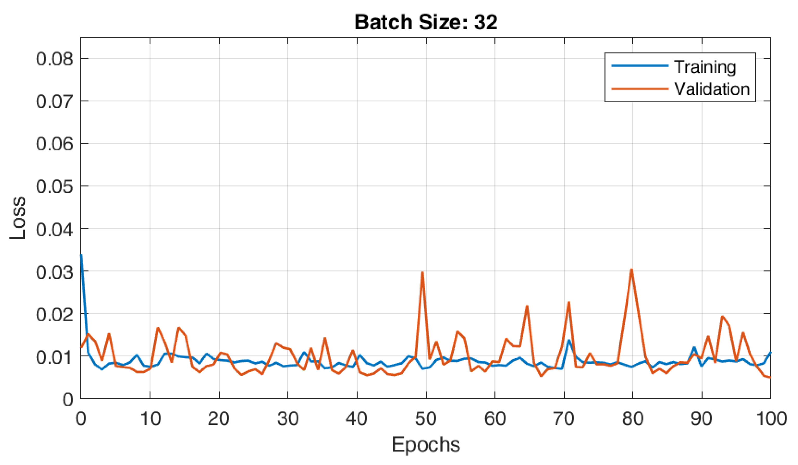
The RBFNN model with 19 centroids and 12 parameters was trained with different batch sizes, i.e., 8, 16, and 32. The converging characteristics of the RBFNN architecture for various batch sizes—8, 16, and 32—are shown in Figure 7, Figure 8 and Figure 9, respectively. According to observations, the RBFNN model that was trained with batch size 32 had a minimal validation loss of 0.0065. Additionally, there was reduced variance between the errors in the training and validation phases, indicating that the model was well trained and free of under- and over-fit issues.

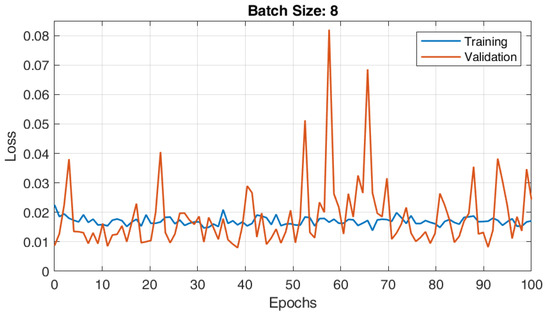
Figure 7. Training and validation plots of RBFNN for load forecasting with batch size 8.

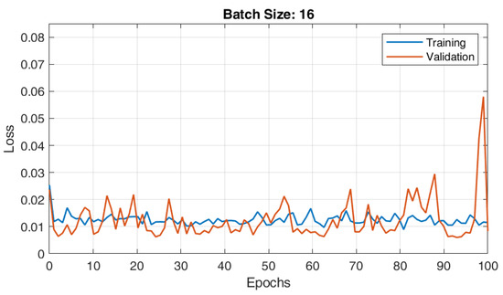
Figure 8. Training and validation plots of RBFNN for load forecasting with batch size 16.

Figure 9. Training and validation plots of RBFNN for load forecasting with batch size 32.

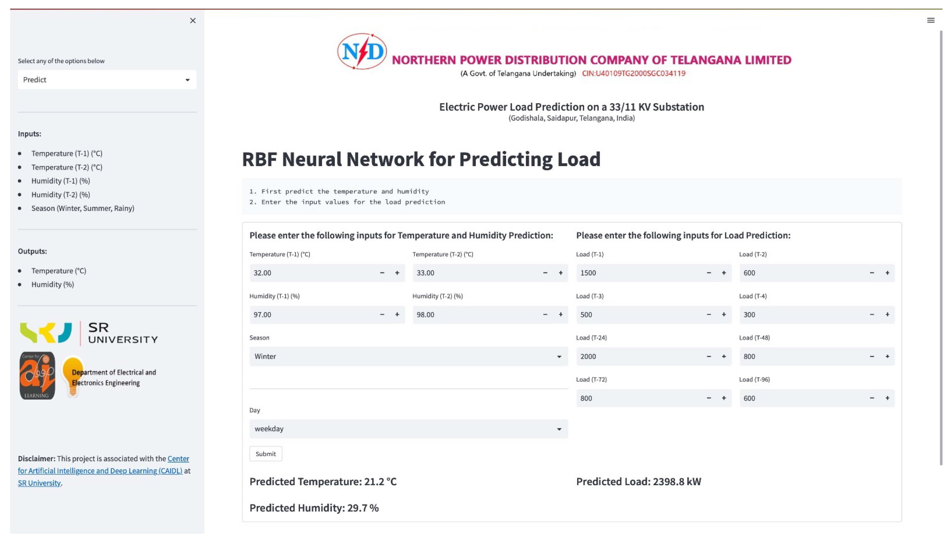
Thus, a web application for forecasting the load associated with the given 33/11 kV substation located in Godishala, Warangal, India, was developed and integrated by running the trained AE-RBFNN combination on the backend; this web application is shown in Figure 10.

Figure 10. Web application to forecast load.

3.4. Comparative Analysis

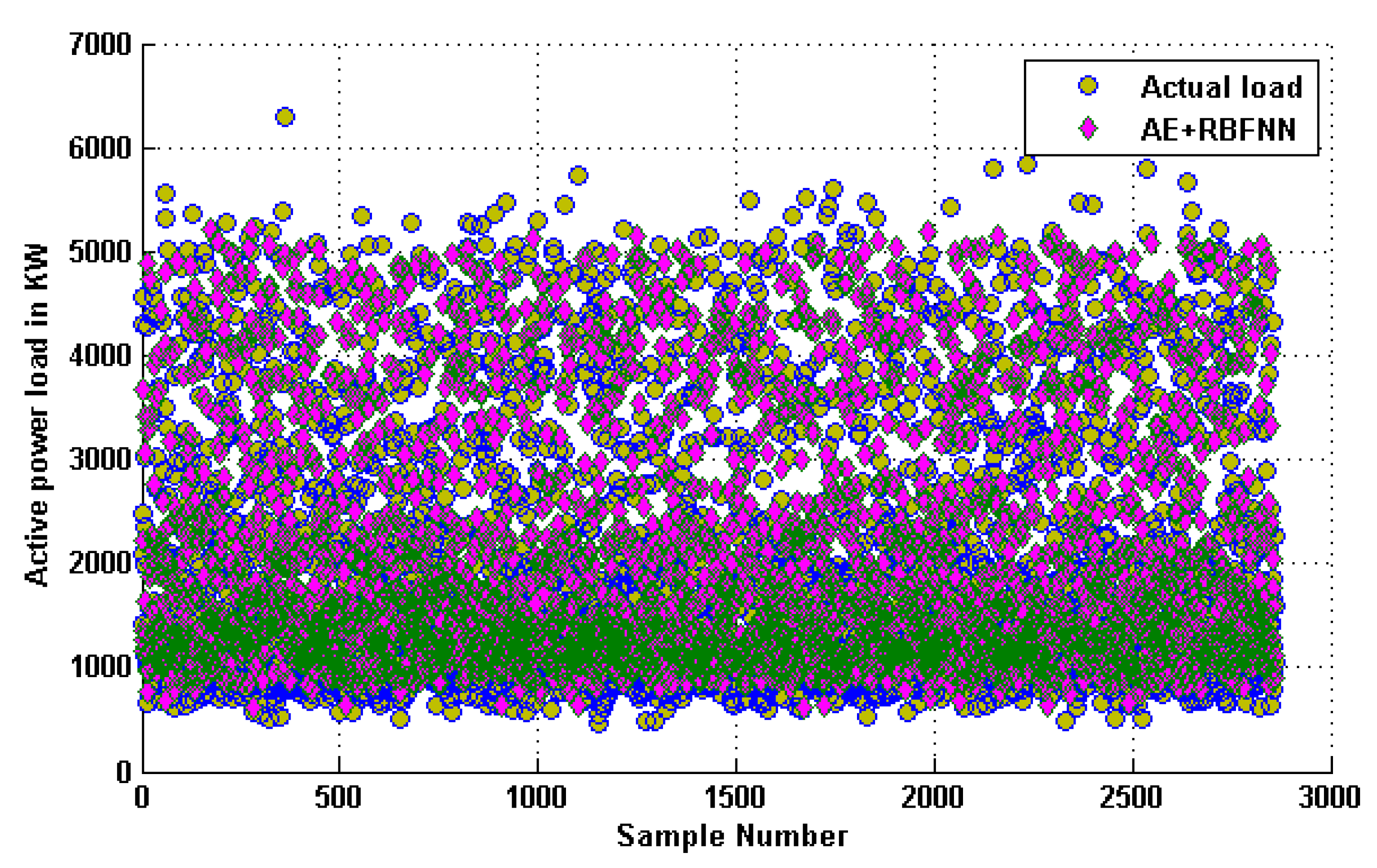
A comparison between the actual load in the training and testing data with the forecast load using the combined AE and RBFNN model is shown in Figure 11 and Figure 12, respectively. It can be observed that the predicted load using our combined AE and RBFNN model is close to the actual load available in the training and testing datasets for most of the samples.

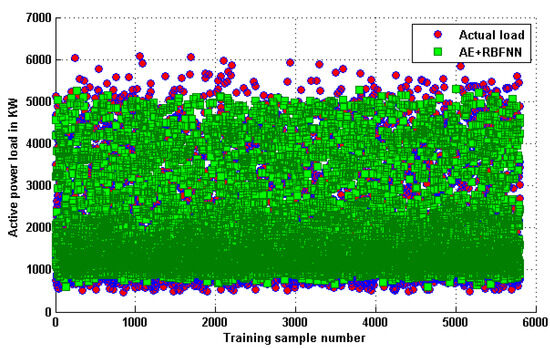
Figure 11. Comparison with actual load available on training dataset.

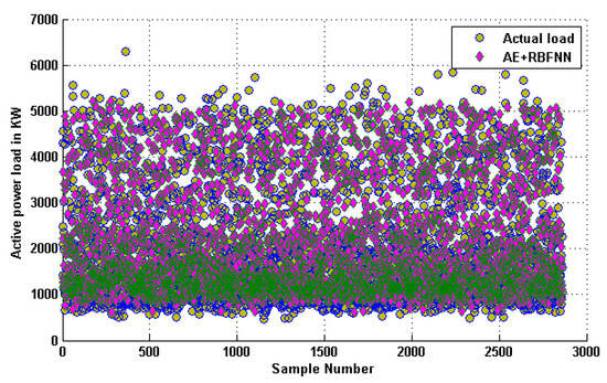
Figure 12. Comparison with actual load available on testing dataset.

The proposed combined AE and RBFNN model for forecasting the load at the given 33/11 kV substation is compared with the RBFNN model without AE in terms of training and validation loss as shown in Figure 13. From Figure 13, it can be observed that the combined AE and RBFNN model performs better than the no-AE RBFNN model, showing less training and a lower validation loss.

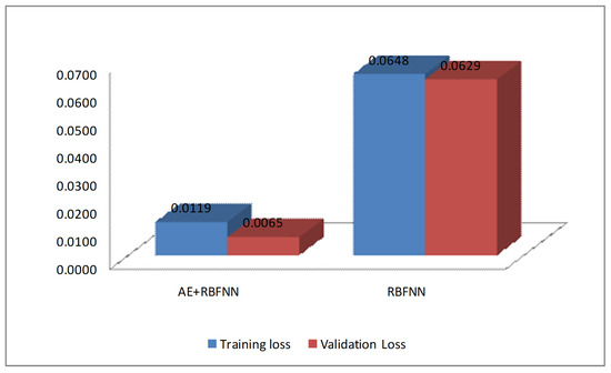
Figure 13. AE + RBFNN vs. RBFNSS.

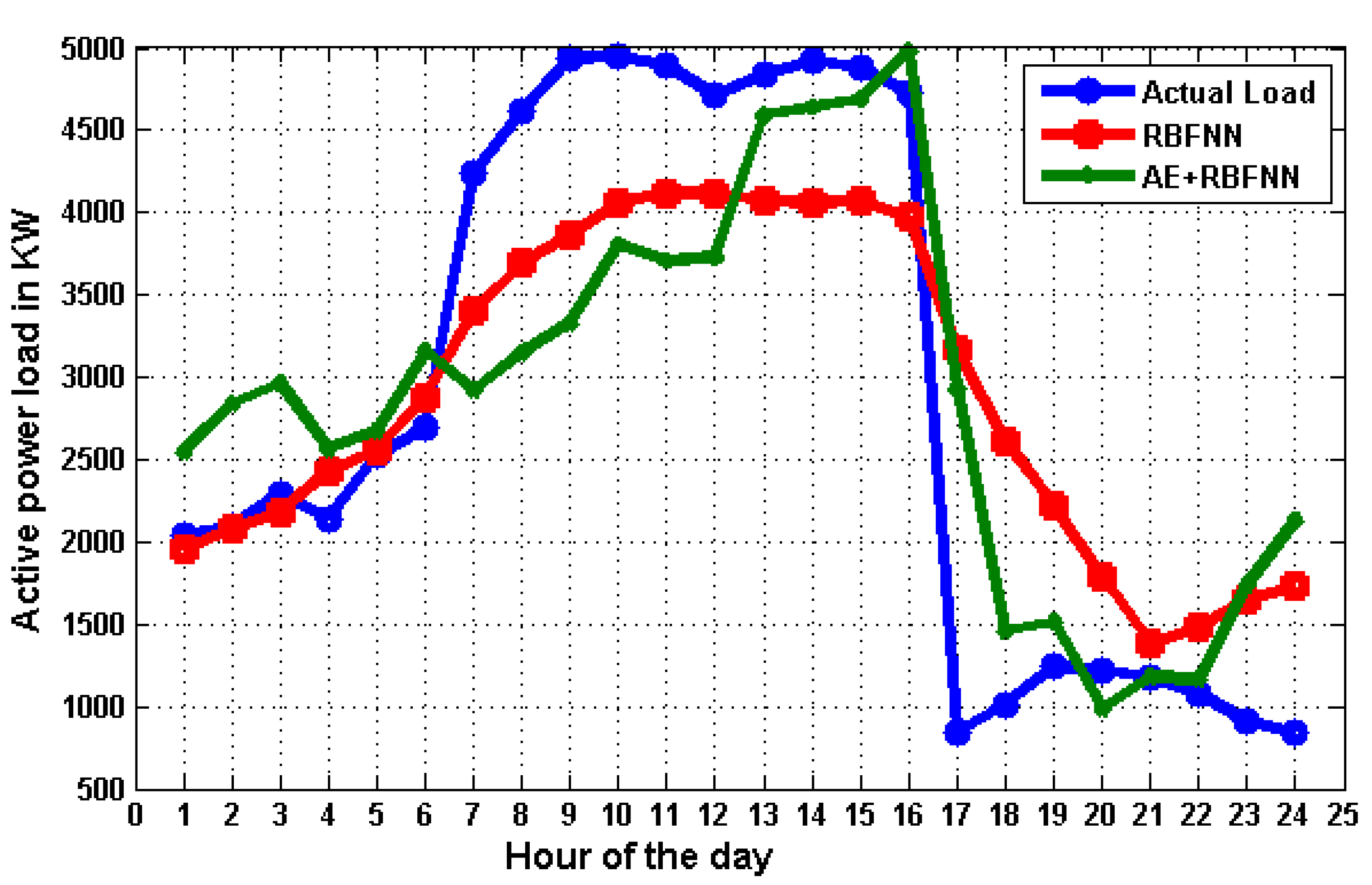
A comparison between the actual load and the load forecasted using the combined AE and RBFNN model is shown in Figure 14, where it can be observed that the load predicted using the combined AE and RBFNN model was closer to the actual load than the load predicted using the only-RBFNN model. A sudden and abnormal deviation of load patterns occurs between the 7th hour and the 16th hour, certainly due to the planning of New Year (2024) celebrations in Warangal, India.

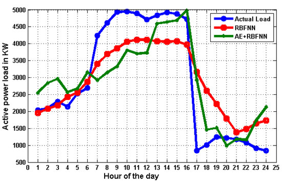
Figure 14. Comparison with actual load on 31 December 2021.

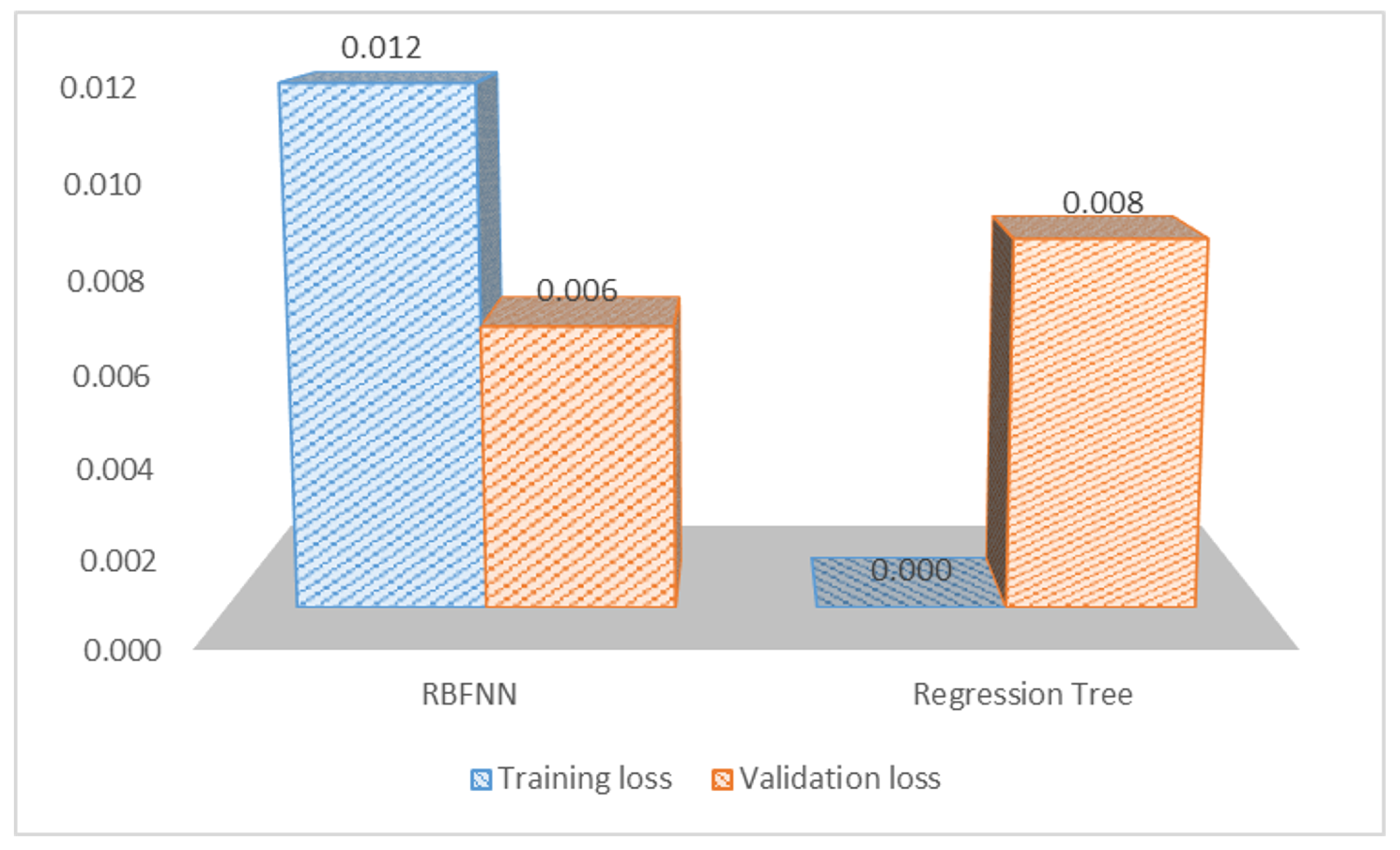
The proposed combined AE and RBFNN model for forecasting the load at the given 33/11 kV substation was validated by comparing it with a regression tree model [42] as shown in Figure 15. Here, it is observed that the regression tree model results in a higher testing loss than the proposed model, while also suffering from over-fitting.

Figure 15. AE + RBFNN vs. regression tree.

The proposed model is also compared in terms of testing loss with the models developed in [21,24] as mentioned in Table 1; the comparison is presented in Table 13. From Table 13, it can be observed that the proposed model predicts the load with the lowest testing loss in comparison with the other models considered.

Table 13. Validation of AE + RBFNN model.

Model	Testing Loss
AE + RBFNN	0.0065
RBFNN [43]	0.0629
Linear Regression Model [21]	0.0075
Regression Tree Model [24]	0.008

4. Conclusions

In this study, a combined AE and RBFNN model was designed to predict the active power load for energy markets one hour ahead of time. AE was utilized as a dimensionality reduction approach to building our light-weight RBFNN model. The AE derives the new features from the original input data. The complexity of the RBFNN model decreases as the number of features retrieved through the AE decreases when compared to the original input features. With respect to the RBFNN model alone, the combined AE and RBFNN model predicts load with higher accuracy. The developed combined AE-RBFNN model was validated by comparing it to the regression tree model in terms of mean square error value, demonstrating that the suggested model is capable of predicting the load one hour in advance with a reduced mean square error value. Temperature and humidity are the two main input factors affecting the load forecasting model; both input variables were forecasted individually using RBFNN. Finally, a web-based application was created to forecast load by executing the suggested combined AE and RBFNN model in the backend. Future studies can extend the physical model, considering more external parameters and exploring different neural structures with respect to different application domains.

References

- Almeshaiei, E.; Soltan, H. A methodology for electric power load forecasting. Alex. Eng. J. 2011, 50, 137–144. [Google Scholar] [CrossRef]
- Vanting, N.B.; Ma, Z.; Jørgensen, B.N. A scoping review of deep neural networks for electric load forecasting. Energy Inform. 2021, 4, 49. [Google Scholar] [CrossRef]
- Giglio, E.; Luzzani, G.; Terranova, V.; Trivigno, G.; Niccolai, A.; Grimaccia, F. An efficient artificial intelligence energy management system for urban building integrating photovoltaic and storage. IEEE Access 2023, 11, 18673–18688. [Google Scholar] [CrossRef]
- Mansoor, M.; Grimaccia, F.; Leva, S.; Mussetta, M. Comparison of echo state network and feed-forward neural networks in electrical load forecasting for demand response programs. Math. Comput. Simul. 2021, 184, 282–293. [Google Scholar] [CrossRef]
- Dagdougui, H.; Bagheri, F.; Le, H.; Dessaint, L. Neural network model for short-term and very-short-term load forecasting in district buildings. Energy Build. 2019, 203, 109408. [Google Scholar] [CrossRef]
- Su, P.; Tian, X.; Wang, Y.; Deng, S.; Zhao, J.; An, Q.; Wang, Y. Recent trends in load forecasting technology for the operation optimization of distributed energy system. Energies 2017, 10, 1303. [Google Scholar] [CrossRef]
- Neusser, L.; Canha, L.N. Real-time load forecasting for demand side management with only a few days of history available. In Proceedings of the IEEE 4th International Conference on Power Engineering, Energy and Electrical Drives, Istanbul, Turkey, 13–17 May 2013; pp. 911–914. [Google Scholar]
- Jahromi, A.J.; Mohammadi, M.; Afrasiabi, S.; Afrasiabi, M.; Aghaei, J. Probability density function forecasting of residential electric vehicles charging profile. Appl. Energy 2022, 323, 119616. [Google Scholar] [CrossRef]
- Massaoudi, M.; S. Refaat, S.; Abu-Rub, H.; Chihi, I.; Oueslati, F.S. PLS-CNN-BiLSTM: An end-to-end algorithm-based Savitzky–Golay smoothing and evolution strategy for load forecasting. Energies 2020, 13, 5464. [Google Scholar] [CrossRef]
- Yin, L.; Xie, J. Multi-temporal-spatial-scale temporal convolution network for short-term load forecasting of power systems. Appl. Energy 2021, 283, 116328. [Google Scholar] [CrossRef]
- Syed, D.; Abu-Rub, H.; Ghrayeb, A.; Refaat, S.S.; Houchati, M.; Bouhali, O.; Bañales, S. Deep learning-based short-term load forecasting approach in smart grid with clustering and consumption pattern recognition. IEEE Access 2021, 9, 54992–55008. [Google Scholar] [CrossRef]
- Munkhammar, J.; van der Meer, D.; Widén, J. Very short term load forecasting of residential electricity consumption using the Markov-chain mixture distribution (MCM) model. Appl. Energy 2021, 282, 116180. [Google Scholar] [CrossRef]
- Guo, W.; Che, L.; Shahidehpour, M.; Wan, X. Machine-Learning based methods in short-term load forecasting. Electr. J. 2021, 34, 106884. [Google Scholar] [CrossRef]
- Timur, O.; Üstünel, H.Y. Short-Term Electric Load Forecasting for an Industrial Plant Using Machine Learning-Based Algorithms. Energies 2025, 18, 1144. [Google Scholar] [CrossRef]
- Eskandari, H.; Imani, M.; Moghaddam, M.P. Convolutional and recurrent neural network based model for short-term load forecasting. Electr. Power Syst. Res. 2021, 195, 107173. [Google Scholar] [CrossRef]
- Guo, W.; Liu, S.; Weng, L.; Liang, X. Power Grid Load Forecasting Using a CNN-LSTM Network Based on a Multi-Modal Attention Mechanism. Appl. Sci. 2025, 15, 2435. [Google Scholar] [CrossRef]
- Perçuku, A.; Minkovska, D.; Hinov, N. Enhancing Electricity Load Forecasting with Machine Learning and Deep Learning. Technologies 2025, 13, 59. [Google Scholar] [CrossRef]
- Cao, W.; Liu, H.; Zhang, X.; Zeng, Y.; Ling, X. Short-Term Residential Load Forecasting Based on the Fusion of Customer Load Uncertainty Feature Extraction and Meteorological Factors. Sustainability 2025, 17, 1033. [Google Scholar] [CrossRef]
- Sheng, Z.; Wang, H.; Chen, G.; Zhou, B.; Sun, J. Convolutional residual network to short-term load forecasting. Appl. Intell. 2021, 51, 2485–2499. [Google Scholar] [CrossRef]
- Hong, T.; Pinson, P.; Fan, S.; Zareipour, H.; Troccoli, A.; Hyndman, R.J. Probabilistic energy forecasting: Global energy forecasting competition 2014 and beyond. Int. J. Forecast. 2016, 32, 896–913. [Google Scholar] [CrossRef]
- Veeramsetty, V.; Mohnot, A.; Singal, G.; Salkuti, S.R. Short term active power load prediction on a 33/11 kv substation using regression models. Energies 2021, 14, 2981. [Google Scholar] [CrossRef]
- Li, B.; Liao, Y.; Liu, S.; Liu, C.; Wu, Z. Research on Short-Term Load Forecasting of LSTM Regional Power Grid Based on Multi-Source Parameter Coupling. Energies 2025, 18, 516. [Google Scholar] [CrossRef]
- Zhao, Y.; Li, J.; Chen, C.; Guan, Q. A Diffusion–Attention-Enhanced Temporal (DATE-TM) Model: A Multi-Feature-Driven Model for Very-Short-Term Household Load Forecasting. Energies 2025, 18, 486. [Google Scholar] [CrossRef]
- Veeramsetty, V.; Sai Pavan Kumar, M.; Salkuti, S.R. Platform-Independent Web Application for Short-Term Electric Power Load Forecasting on 33/11 kV Substation Using Regression Tree. Computers 2022, 11, 119. [Google Scholar] [CrossRef]
- Abumohsen, M.; Owda, A.Y.; Owda, M. Electrical load forecasting using LSTM, GRU, and RNN algorithms. Energies 2023, 16, 2283. [Google Scholar] [CrossRef]
- Subray, S.; Tschimben, S.; Gifford, K. Towards Enhancing Spectrum Sensing: Signal Classification Using Autoencoders. IEEE Access 2021, 9, 82288–82299. [Google Scholar] [CrossRef]
- Atienza, R. Advanced Deep Learning with Keras: Apply Deep Learning Techniques, Autoencoders, GANs, Variational Autoencoders, Deep Reinforcement Learning, Policy Gradients, and More; Packt Publishing Ltd.: Birmingham, UK, 2018. [Google Scholar]
- Veeramsetty, V.; Kiran, P.; Sushma, M.; Babu, A.M.; Rakesh, R.; Raju, K.; Salkuti, S.R. Active power load data dimensionality reduction using autoencoder. In Power Quality in Microgrids: Issues, Challenges and Mitigation Techniques; Springer: Berlin/Heidelberg, Germany, 2023; pp. 471–494. [Google Scholar]
- Wurzberger, F.; Schwenker, F. Learning in deep radial basis function networks. Entropy 2024, 26, 368. [Google Scholar] [CrossRef]
- Yu, Q.; Hou, Z.; Bu, X.; Yu, Q. RBFNN-based data-driven predictive iterative learning control for nonaffine nonlinear systems. IEEE Trans. Neural Networks Learn. Syst. 2019, 31, 1170–1182. [Google Scholar] [CrossRef]
- Liu, J. Radial Basis Function (RBF) Neural Network Control for Mechanical Systems: Design, Analysis and Matlab Simulation; Springer Science & Business Media: Berlin/Heidelberg, Germany, 2013. [Google Scholar]
- Lu, Y.; Cheung, Y.M.; Tang, Y.Y. Self-adaptive multiprototype-based competitive learning approach: A k-means-type algorithm for imbalanced data clustering. IEEE Trans. Cybern. 2019, 51, 1598–1612. [Google Scholar] [CrossRef]
- Lillicrap, T.P.; Santoro, A.; Marris, L.; Akerman, C.J.; Hinton, G. Backpropagation and the brain. Nat. Rev. Neurosci. 2020, 21, 335–346. [Google Scholar] [CrossRef]
- Kandilogiannakis, G.; Mastorocostas, P.; Voulodimos, A.; Hilas, C. Short-Term Load Forecasting of the Greek Power System Using a Dynamic Block-Diagonal Fuzzy Neural Network. Energies 2023, 16, 4227. [Google Scholar] [CrossRef]
- Zaini, F.A.; Sulaima, M.F.; Razak, I.A.W.A.; Othman, M.L.; Mokhlis, H. Improved Bacterial Foraging Optimization Algorithm with Machine Learning-Driven Short-Term Electricity Load Forecasting: A Case Study in Peninsular Malaysia. Algorithms 2024, 17, 510. [Google Scholar] [CrossRef]
- Ng, W.W.; Xu, S.; Wang, T.; Zhang, S.; Nugent, C. Radial basis function neural network with localized stochastic-sensitive autoencoder for home-based activity recognition. Sensors 2020, 20, 1479. [Google Scholar] [CrossRef]
- Yang, Y.; Wang, P.; Gao, X. A novel radial basis function neural network with high generalization performance for nonlinear process modelling. Processes 2022, 10, 140. [Google Scholar] [CrossRef]
- Veeramsetty, V.; Kiran, P.; Sushma, M.; Salkuti, S.R. Weather Forecasting Using Radial Basis Function Neural Network in Warangal, India. Urban Sci. 2023, 7, 68. [Google Scholar] [CrossRef]
- Lee, C.M.; Ko, C.N. Short-term load forecasting using adaptive annealing learning algorithm based reinforcement neural network. Energies 2016, 9, 987. [Google Scholar] [CrossRef]
- Liu, P.; Zheng, P.; Chen, Z. Deep learning with stacked denoising auto-encoder for short-term electric load forecasting. Energies 2019, 12, 2445. [Google Scholar] [CrossRef]
- Vaccaro Benet, P.; Ugalde-Ramírez, A.; Gómez-Carmona, C.D.; Pino-Ortega, J.; Becerra-Patiño, B.A. Identification of Game Periods and Playing Position Activity Profiles in Elite-Level Beach Soccer Players Through Principal Component Analysis. Sensors 2024, 24, 7708. [Google Scholar] [CrossRef]
- Tsionas, M.; Assaf, A.G. Regression trees for hospitality data analysis. Int. J. Contemp. Hosp. Manag. 2023, 35, 2374–2387. [Google Scholar] [CrossRef]
- Song, C.Y. A Study on Learning Parameters in Application of Radial Basis Function Neural Network Model to Rotor Blade Design Approximation. Appl. Sci. 2021, 11, 6133. [Google Scholar] [CrossRef]
Disclaimer/Publisher’s Note: The statements, opinions and data contained in all publications are solely those of the individual author(s) and contributor(s) and not of MDPI and/or the editor(s). MDPI and/or the editor(s) disclaim responsibility for any injury to people or property resulting from any ideas, methods, instructions or products referred to in the content. |
© 2025 by the authors. Licensee MDPI, Basel, Switzerland. This article is an open access article distributed under the terms and conditions of the Creative Commons Attribution (CC BY) license (https://creativecommons.org/licenses/by/4.0/).