Abstract
Ship maneuverability models are typically defined by three degrees of freedom: surge, sway, and yaw. However, patrol vessels operating in riverine environments often exhibit significant roll motion during course changes, necessitating the inclusion of this dynamic. This study develops interpretable machine learning models capable of predicting vessel behavior in four degrees of freedom (4-DoF): surge, sway, yaw, and roll. A dataset of 125 h of simulated maneuvers was employed, including 29 h of out-of-distribution (OOD) conditions to test model generalization. Four models were implemented and compared over a 15-step prediction horizon: linear regression, third-order polynomial regression, a state-space model obtained via the N4SID algorithm, and an AutoRegressive model with eXogenous inputs (ARX). Results demonstrate that all models captured the essential vessel dynamics, with the state-space model achieving the best overall performance (e.g., NMSE = 0.0246 for surge velocity on test data and 0.0499 under OOD conditions). Variable-wise, surge and sway showed the lowest errors, roll rate remained stable, and yaw rate was the most sensitive to distribution shifts. Model-wise, the ARX model achieved the lowest NMSE for surge prediction (0.0149), while regression-based models provided interpretable yet less accurate alternatives. Multi-horizon evaluation (1-, 5-, 15-, and 30-step) under OOD conditions confirmed a consistent monotonic degradation across models. These findings validate the feasibility of using interpretable machine learning models for predictive control, autonomous navigation, and combat scenario simulation in riverine operations.
1. Introduction
Accurate prediction and control of the trajectory, speed, and acceleration of a ship are crucial for effective maneuvering, especially in the context of the design of autonomous ship navigation systems and collision avoidance strategies [1]. In the literature, there is a wide range of maneuvering models, generally classified into hydrodynamic and mathematical response models. Hydrodynamic models, such as the Abkowitz model [2] and the Mathematical Ship Maneuvering Group (MMG) models [3], focus on capturing the physical dynamics of the vessel. In contrast, response models directly relate the motion of a ship to the actions of steering, with the first- and second-order models of Nomoto [4,5] and the nonlinear Nomoto model [6] being popular choices due to their simplicity, which are often used for the control of the direction of the ship using PID controllers, as they bypass the need to calculate hydrodynamic derivatives.
Hydrodynamic models are typically constructed with three or four degrees of freedom (4-DoF) [7,8,9]. Although some studies suggest the superiority of 4-DoF structures over 1-DoF models [10], this is not a strict rule. Although hydrodynamic models offer high precision, they are complex because of the large number of parameters and nonlinearities involved. Consequently, various methods for parameter estimation, including theoretical calculations (white-box models), captive model testing, and Computational Fluid Dynamics (CFD) [11], have been explored. System identification, in particular, has gained attention with advances in artificial intelligence and autonomous learning algorithms [12,13].
This paper aims to develop two multistep prediction models using system identification: a linear regression model, a third-order polynomial regression model, a state-space model, and an ARX model. The models will be evaluated over a prediction horizon of , with the Normalized Mean Squared Error (NMSE) serving as the primary error metric.
This paper is structured into several key sections. The Section 2 highlights the study’s advances, including the integration of roll motion and the development of two interpretable models. Section 3 reviews existing research on system identification and hybrid modeling approaches. In Section 5, the dataset is described, detailing its division and the modeling techniques applied. Section 6 presents the results of the developed models, including responses and error metrics. Finally, Section 7 summarizes the effectiveness of models in predicting vessel dynamics.
2. Contributions
By incorporating roll motion into traditionally 3-DoF models, research improves understanding of vessel dynamics. Two interpretable models are developed, evaluated, and validated through error metrics and residual analysis, demonstrating their robustness and accuracy in predicting vessel behavior in real-world applications. These contributions offer valuable insights for improving predictive control systems and autonomous navigation.
- Unlike traditional 3-DoF approaches, this work incorporates roll dynamics into a 4-DoF framework, enabling a more accurate and realistic representation of patrol vessel behavior during sharp course changes.
- Linear regression, third-order polynomial regression, state-space (via N4SID), and ARX models were implemented and systematically compared. This provides a spectrum of approaches ranging from highly interpretable to more data-driven, offering practical options for different control applications.
- All models successfully captured the dynamics of the vessel over a 15-step horizon. The state-space model consistently delivered the lowest NMSE and strongest generalization across both validation and out-of-distribution datasets, while the ARX model excelled at forecasting specific variables under complex dynamic conditions.
- Although regression-based models showed slightly higher errors, they remain valuable due to their simplicity and transparency, making them suitable for real-time implementation in predictive controllers. In contrast, the state-space and ARX models offer stronger predictive accuracy, especially under unseen operating conditions.
- By evaluating the models against 29 h of maneuvers outside the training distribution, the study demonstrates resilience to variations in propulsion and environmental conditions, supporting future deployment in real-world autonomous navigation and combat training scenarios.
3. Related Works
Identification of a system involves developing mathematical models from experimental input-output data to replicate its dynamic behavior. This process includes several stages: optimal experimental design, data preprocessing, selection of the model structure, parameter estimation, and model validation. A key method for generating maneuvering coefficients is the Planar Motion Mechanism (PMM) test [14]. For example, ref. [15] employed a modified regression model using Least Squares Support Vector Machines (LS-SVM) to derive hydrodynamic derivatives for an Abkowitz-type model, incorporating wavelet threshold denoising to filter noise. Model validation included standard tests such as the zigzag, zigzag, and 35 turning-circle tests. Similarly, ref. [16] applied system identification to create a 4-DoF maneuvering model for a surface combatant in intact and damaged conditions.
Theoretical models, often called white-box models, provide interpretability by explicitly describing the relationships between variables, but they require a deep understanding of the underlying physics. In contrast, black-box models, such as Artificial Neural Networks (ANNs) and Support Vector Machines (SVMs) [17], offer high accuracy but lack interpretability. Hybrid models attempt to bridge this gap by combining white-box and black-box methods to improve accuracy while retaining some interpretability. For example, the KINN model [18] uses a Deep Neural Network (DNN) to correct the residual error of a theoretical model.
Several examples of hybrid and gray-box models exist in the literature. In [19], an interpretable model based on parameters from PMM tests was developed to predict the maneuvering capabilities of ships with azimuth thrusters. Another example is the gray-box model by [20], which used Ordinary Least Squares (OLS) to estimate hydrodynamic derivatives, with Extended Kalman Filters (EKF) and Rauch-Tung-Striebel (RTS) smoothers to address noise. Multiple models, including linear and modified Abkowitz models, were considered for selection.
Additionally, ref. [21] derived parametric and non-parametric gray-box models and black-box models to predict ship dynamics. These models used a combination of past surge speed, sway speed, yaw, roll, and rudder angle as input to predict future dynamics. Other works, such as [22], have focused on one-step and multistep forecast models for ship dynamics, using prediction horizons ranging from 1 to 60 time steps.
Mathematical models capable of predicting future values play a critical role in the design of predictive controllers. However, models derived solely from simulations can lead to low-precision predictions and unstable controller behavior, underscoring the importance of using real-time experimental data and accounting for external disturbances [23].
4. Methodology
The methodological framework proposed in this research, presented in Figure 1, integrates simulation-based data generation, systematic preprocessing, and machine learning-driven system identification to predict the maneuverability of a 4-DoF river combat patrol vessel. The process begins with the execution of high-fidelity simulation tests that incorporate both ship parameters (propeller shaft speed, propeller azimuth angles) and environmental factors (wind speed and direction, represented through attack angles). These simulations produced 125 h of time-series data, of which 29 h corresponded to out-of-distribution (OOD) scenarios, enabling evaluation of model generalization.
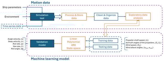
Figure 1.
Methodological framework for 4-DoF ship maneuverability model identification.
The generated data were then processed, stored, and cleaned and organized, including the identification of missing or duplicated values, normalization of variable ranges, and division into training, testing, validation, and OOD subsets. The exploratory data analysis was then performed to characterize the correlations among the variables and to assess the dynamics of the ship under routine and OOD conditions. This stage laid the foundation for selecting appropriate modeling strategies and highlighted the influence of propulsion and environmental inputs on the vessel’s dynamic response.
Four predictive models were implemented to capture vessel dynamics: (i) Linear regression model; (ii) Third-order polynomial regression model; (iii) AutoRegressive model with eXogenous inputs (ARX), and (iv) State-space model identified through the N4SID algorithm. These models were chosen to provide a spectrum of interpretability and predictive capacity, ranging from simple baseline predictors to more complex dynamic formulations capable of reconstructing internal vessel states. Training and testing of the models were carried out on the prepared datasets, with a prediction horizon fixed at 15 steps ahead.
Model validation was performed using the NMSE as the primary evaluation metric. A comparative analysis was conducted across the training, validation, and OOD datasets, supplemented by time-series plots of predicted versus measured trajectories. This allowed both quantitative and qualitative assessment of model accuracy and robustness. Results confirmed that while regression-based models offered interpretability and computational efficiency, the ARX model excelled in predicting autoregressive dynamics such as surge velocity, and the state-space model achieved the strongest overall generalization across both routine and OOD scenarios.
Finally, the methodological proposal emphasizes the scalability of the developed framework. By integrating system identification with interpretable machine learning, the approach provides a reproducible basis for modeling vessel maneuverability, which can be extended to other motion platforms with varying degrees of freedom. Moreover, the combination of rigorous preprocessing, structured validation, and interpretable modeling ensures applicability not only to predictive control and autonomous navigation, but also to experimental testbeds and combat training simulations in complex riverine environments.
5. Materials and Methods
The methodological framework of this study was designed to integrate data-driven modeling techniques with the principles of system identification to capture the maneuverability characteristics of a river patrol vessel under realistic operating conditions. This section describes the dataset employed, including its composition, preprocessing, and division into training, validation, and OOD subsets. Then it outlines the modeling strategies implemented, namely linear regression, polynomial regression, state-space representation, and ARX models with AR inputs. Each method was selected to provide a balance between interpretability and predictive accuracy, enabling a rigorous evaluation of their capacity to forecast vessel dynamics across multiple degrees of freedom. The subsequent subsections present the dataset structure, the modeling approaches, and the validation procedures used to assess model performance.
5.1. Dataset
The dataset consists of 125 h of simulation data on the motion of a patrol boat designed by Pérez et al. [24] under various sea states. The samples were taken at a rate of 1 Hz, performing random maneuvers in 4-DoF, i.e., surge, sway, yaw, roll. The original boat has been expanded by incorporating two symmetrically placed rudder propellers and wind force simulations following the Isherwood model [25]. Wind-induced waves were generated using the JONSWAP spectrum [26].
It is important to emphasize that the dataset used in this study consists of randomly generated maneuvering sequences rather than standardized International Maritime Organization-IMO (compliant tests such as turning-circle, zigzag, or spiral maneuvers. Because canonical maneuverability indices—such as turning diameter, tactical diameter, advance, transfer, or yaw response times) require specific and repeatable control protocols, these metrics cannot be extracted from the available dataset. The focus of the present work is therefore on evaluating multistep dynamic prediction accuracy under varying propulsion and environmental conditions, rather than on computing classical maneuverability performance indicators.
The dataset is divided into two parts: one corresponds to the routine operations dataset, totaling 96 h, and the other to an OOD dataset, totaling 29 h. The routine operations dataset is divided into three groups with the following percentages: 60-10-30, corresponding to training, test, and validation data. The OOD dataset is only used for testing purposes.
The dataset is used to obtain models that predict several steps ahead using machine learning methods. The following inputs or predictor variables are considered for model generation: speeds of the axes of both propeller helices (n), azimuth angles of the propellers (: left and right), wind speed (), and angle of attack (, ). The output variables include the surge speed (u), the sway speed (v), angular velocity of roll (p), yaw rate (r), and the roll angle () [27].
It is important to note that the dataset employed in this study consists exclusively of high-fidelity simulated maneuvers. This choice allows controlled exploration of 4-DoF dynamics under a wide range of propulsion and environmental disturbances that are difficult to replicate systematically in field trials. Simulation-based evaluation is therefore used as a foundational step before transitioning to model identification using real ship trials. The use of simulated data therefore serves as an essential foundational stage, allowing the comparative evaluation of interpretable identification models before transitioning to validation with real ship maneuvering experiments.
The correlation matrix between the variables (training data) is shown in Figure 2.
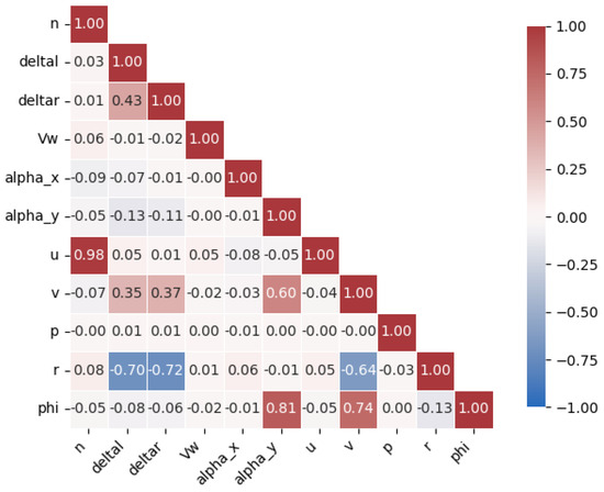
Figure 2.
Correlation matrix between variables (training data).
Initially, we examined the distributions of input variables across the training, test, validation, and OOD datasets, as shown in Figure 3.
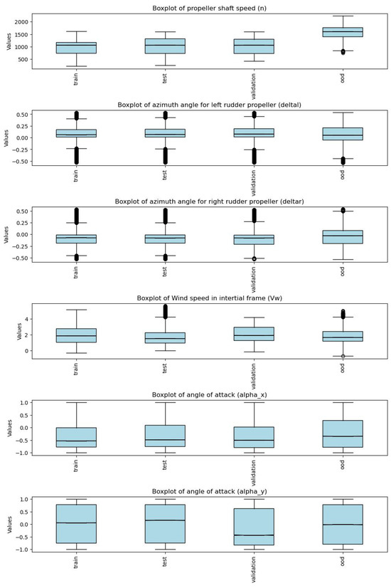
Figure 3.
Distribution of input data in each group: training, test, validation, and out-of-distribution (OOD).
The value of the variable n in the OOD dataset deviated from the range and median observed in the other datasets (training, test, and validation), representing the primary source of shift in the OOD distribution. A quantitative analysis revealed that shaft speed in the training set spans from 226 to 1612 rpm, whereas the OOD dataset reaches 2233 rpm, with 47.9% of its samples lying outside this interval. In contrast, the ranges of , , , , and remain almost entirely within the training support, with less than 1% of samples falling outside their respective ranges.
5.2. Modeling
Figure 4 shows the six degrees of freedom of the vessel. The data set used to train the models was collected from random maneuvers in 4 degrees of freedom (surge, sway, roll rate, yaw rate, and roll angle).
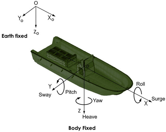
Figure 4.
Six degrees of freedom ship motions.
Based on the dataset mentioned above, this study obtains four models to predict the surge speed (u), the sway speed (v), roll rate (p), the yaw rate (r), and the roll angle () variables; using as input variables the speeds of the propeller shaft speed (n), azimuth angles of the propellers ( and ), wind speed () and the wind angles of attack ( and ). Figure 5 shows the input-output relations.
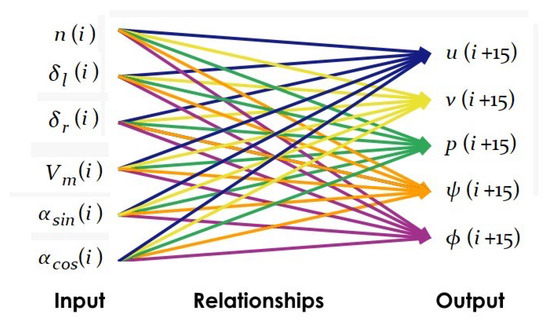
Figure 5.
Input/Output Model.
It should be noted that all experiments in this study were conducted in an offline computational environment using the simulated 4-DoF maneuvering dataset. Real-time execution and hardware-in-the-loop evaluation were beyond the scope of the present work, as the objective here was to establish a controlled comparison of interpretable identification models under routine and OOD operating conditions. Nevertheless, the computational structure of all four models—linear and polynomial regression, ARX, and state-space—is lightweight and compatible with embedded implementation, since each relies on closed-form matrix operations with low execution overhead. These characteristics make them suitable candidates for real-time testing in future hardware-oriented validation stages.
6. Results
This section presents the outcomes of the four predictive models developed for the 4-DoF maneuverability analysis of the patrol vessel. The performance of linear, polynomial, state-space, and ARX models is evaluated using NMSE as the primary metric across training, validation, and OOD datasets. To account for statistical significance, bootstrap resampling with 10 runs was employed to estimate the mean and standard deviation of the NMSE residuals for each dataset. In addition to these quantitative error measures, graphical comparisons of predicted and observed time series are provided to illustrate the models’ ability to capture vessel dynamics under varying operating conditions. The results highlight not only the relative accuracy of each modeling approach but also their robustness and generalization capabilities, which are critical for real-world predictive control and autonomous navigation applications.
The evaluation metrics employed in this study (i.e., NMSE, bootstrap-based variability estimates, and graphical time-series comparisons) align with the primary objective of assessing predictive accuracy and generalization under varying propulsion and environmental inputs. Since the dataset consists of non-standardized maneuvering sequences produced by random excitation, it does not include the structured control protocols required to compute domain-specific maneuverability indices such as turning diameter, tactical diameter, advance, transfer, or yaw response time. For this reason, trajectory-level dynamic prediction metrics were selected as the most appropriate and consistent tools for comparing the four model classes evaluated in this work.
6.1. Linear Regression Model
To establish the linear regression model, the intercept values for each predicted variable were first obtained, as shown in Equation (1). Subsequently, the coefficients associated with the input variables were estimated, and their values are reported in Table 1.

Table 1.
Linear model coefficients.
These coefficients, together with the intercepts, define the full mathematical formulation of the linear model expressed in Equation (2), which relates propulsion and environmental input to surge velocity (u), sway velocity (v), roll rate (p), yaw rate (r), and the roll angle () of the vessel over a 15-step prediction horizon. To assess predictive accuracy, the NMSE was calculated according to Equation (3), which allows for a quantitative evaluation of the performance of the model in the training, validation, and OOD datasets.
The linear regression model obtained a determination coefficient of , indicating that approximately 60% of the variance in the vessel’s dynamic response is explained by the selected input variables. Although this value reflects only moderate predictive ability, it shows the model’s ability to capture the main trends of system dynamics with a relatively simple structure. To provide a more rigorous performance assessment, the NMSE was calculated for each output variable using Equation (3). The resulting NMSE values for all output variables across the training, validation, and OOD datasets are summarized in Table 2, which enables a consistent comparison of predictive accuracy and highlights the model’s ability to generalize beyond the conditions used for parameter estimation. Within the broader research framework, these results highlight the relevance of interpretable models as baseline predictors. Although less precise than nonlinear structures, linear regression offers transparency and computational efficiency. These properties make it suitable for rapid prototyping and real-time monitoring.
where is the observed value ith, is the predicted value corresponding, and n is the number of observations. Figure 6 presents the approximation graphs for each variable in the test and OOD datasets.
Table 2.
NMSE linear model results.
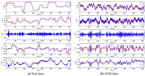
Figure 6.
Linear model validation.
Figure 6 illustrates the comparison between the observed and predicted vessel dynamics obtained with the linear regression model for both the test dataset (Figure 6a) and the OOD dataset (Figure 6b). In the test dataset, the predicted trajectories closely follow the measured responses for u, v, p, r, and , indicating an adequate fit under in-distribution conditions.
The residuals obtained with the linear regression model are reported in Table 3, which shows their mean and standard deviation derived from the prediction errors computed independently for each dataset. This data further confirms this behavior, with mean errors remaining very close to zero across all datasets. This finding confirms that the linear approximation does not introduce any relevant systematic bias in the analyzed outputs. In particular, for , , , , and , the mean residuals remain on the order of to in the training, testing, and validation sets, demonstrating satisfactory statistical consistency of the estimator.
Table 3.
Residuals mean ± standard deviation for the linear regression model.
Regarding error dispersion, the standard deviation values within the in-distribution datasets (Train, Test, and Validation) remain within narrow ranges, indicating reproducible predictions with low variability under nominal operating conditions. By contrast, evaluation on the out-of-distribution (OOD) dataset reveals a clear increase in variance, most notably for and , reflecting reduced accuracy under extreme maneuvering scenarios. This aligns with the limitations of linear models, where generalization falters amid dominant nonlinear hydrodynamic effects.
6.2. Polynomial Regression Model
The third-degree polynomial regression model was developed to extend the linear formulation by incorporating nonlinear interactions between inputs and outputs, thereby improving predictive accuracy.
Figure 7 further illustrates the performance of the polynomial model for both the test dataset (Figure 7a) and the OOD dataset (Figure 7b). In the test dataset, the predicted trajectories align more closely with the measured responses than those from the linear model, capturing both amplitude and phase variations more accurately. Under OOD conditions, larger deviations are observed, especially in v and r, reflecting the increased difficulty in generalizing polynomial models beyond the training distribution. Nevertheless, the predictions preserve the overall temporal structure of the vessel dynamics, indicating that polynomial regression provides a valuable compromise between enhanced accuracy and interpretability within the broader modeling framework.
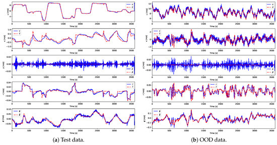
Figure 7.
Third-degree polynomial model validation.
As reported in Table 4, this approach achieved lower NMSE values than the linear model in most state variables, particularly for u and p, with test errors of 0.0295 and 0.0363, respectively, demonstrating the benefit of including nonlinear interactions.
Table 4.
NMSE Polynomial Model Results.
The residuals obtained with the polynomial regression model are reported in Table 5, which shows their mean and standard deviation derived from the prediction errors computed independently for each dataset. This data indicates that the model accurately reproduces the mean behavior of all output variables in the in-distribution datasets, as the mean residuals remain very close to zero in the training, testing, and validation sets. However, in the out-of-distribution (OOD) dataset, noticeable biases emerge, particularly for and , where mean residuals reach orders of to . These values are consistent with the previously reported performance metrics. For , , , , and , the mean residuals remain on the order of to for the training, testing, and validation sets, confirming the absence of relevant systematic bias under nominal conditions.
Table 5.
Residuals mean ± standard deviation for the polynomial regression model.
Regarding error dispersion, the standard deviation values within the in-distribution datasets are moderate and comparable among them, indicating a stable predictive behavior under nominal operating conditions. In the out-of-distribution (OOD) dataset, a noticeable increase in variance is observed for all outputs, particularly for and , reflecting an increased sensitivity under extreme maneuvering scenarios. Nevertheless, the growth of uncertainty remains bounded and is lower than that observed for the strictly linear model, highlighting the greater representational capability of the polynomial approximation.
6.3. AutoRegressive Model with Exogenous Inputs
The ARX model is a well-established data-driven technique in system identification, widely used for time-series forecasting and control design. Unlike purely regression-based approaches, the ARX framework explicitly incorporates temporal dependencies by linking the present value of each output variable not only to contemporaneous inputs but also to its past values. This recursive structure enables the model to capture short-term memory effects and dynamic correlations between successive state of the vessel, making it particularly suitable for predicting ship maneuverability under evolving conditions. In the context of this study, the ARX formulation was applied to all five output variables (i.e., u, v, p, r, and ) using propulsion and wind-related variables as exogenous inputs. Parameter estimation was performed via least-squares optimization, ensuring computational efficiency while preserving the model’s interpretability.
Equations set (4)–(8) present the detailed ARX structures derived for each output variable, where the autoregressive polynomials and the input-dependent polynomials capture both the inherent dynamics of the system and the effect of external forcing terms. Specifically, u, v, p, r, and in Equations (6)–(10), respectively. Together, these formulations illustrate how the recursive integration of past outputs with exogenous propulsion and wind inputs provides a flexible, yet interpretable framework for multistep prediction of ship maneuverability in 4-DoF.
where,
where,
where,
where,
where,
The results, summarized in Table 6, indicate that the ARX model achieved robust predictive performance across both the test and OOD datasets. For the test data, the NMSE values were consistently low, with u reaching 0.0149, the best score among all models considered. This highlights the ability of the ARX structure to exploit temporal correlations for improved short-term forecasting. In Figure 8a, the predicted trajectories closely match the measured responses for all variables, confirming the adequacy of the recursive formulation in capturing the dynamics of the vessel during standard maneuvers. Under OOD conditions (Figure 8b), deviations become more noticeable, particularly in v and r, but the model continues to reproduce the principal oscillatory patterns of the motion of the ship, demonstrating resilience to unseen operating scenarios.
Table 6.
Residuals mean ± standard deviation for the ARX model.
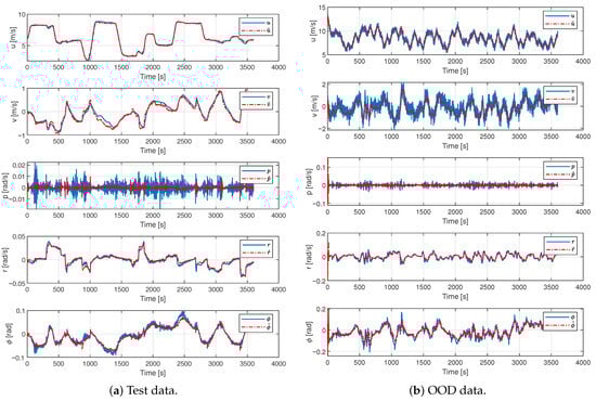
Figure 8.
ARX model validation.
The residual statistics of the ARX model, presented in Table 6, exhibit moderate biases and relatively large variances that remain fairly consistent across all data partitions. Such behavior is common in ARX formulations when applied to multivariable systems with significant dynamic coupling, since the model structure does not explicitly encode cross-variable interactions or nonlinear effects. The surge and sway velocities, and , show mean residuals between approximately and , while the yaw-rate displays a small negative bias; however, these tendencies remain bounded and do not grow in the OOD dataset, indicating stable prediction behavior. The roll rate achieves residual means close to zero, although its variance is still considerable, which is expected for fast angular dynamics under an ARX structure. Overall, the results suggest that while the ARX model captures some aspects of the vessel dynamics, its linear autoregressive structure limits its ability to fully represent the USV’s multivariate, strongly coupled behavior. Such limitations become more apparent when examining the model response in conditions not represented during training. As shown in Figure 8b, although overall trends remain well aligned with the observed dynamics, discrepancies are more pronounced in v and r, where phase lags and amplitude mismatches appear.
From a broader perspective, the results confirm that ARX benefits substantially from its recursive structure, which leverages past states for more accurate short-term forecasting. This advantage is evident in the prediction of surge velocity, where the ARX model achieved the lowest NMSE (0.0149 on test data). However, for variables more strongly influenced by nonlinear hydrodynamic effects, such as r and v, the ARX model exhibits lower precision than the state-space formulation. Despite this, its performance under OOD conditions demonstrates robustness and adaptability, highlighting ARX as a valuable intermediary between simple regression approaches and more complex, higher-dimensional models.
6.4. State-Space Model
The state-space approach offers a mathematically rigorous framework for representing dynamic systems, making it particularly suitable for modeling vessel maneuverability. Unlike regression-based methods, which approximate direct input–output relationships, state-space models reconstruct the system’s internal dynamics using latent state variables. This property is essential when the objective is not only to predict trajectories but also to recreate the underlying dynamic structure of the vessel, thereby enabling scalability to more complex experiments and extended operating scenarios. In this study, the state-space model was identified using the Numerical Subspace System Identification (N4SID) algorithm, which directly derives the state, input, and output matrices (A, B, and C) from the input-output dataset. This methodology ensures that the estimated model closely corresponds to the physics of maneuvering while remaining computationally tractable for predictive applications.
The state of a dynamical system is the smallest set of variables (called state variables) such that knowledge of these variables at , together with knowledge of the input to , completely determines the behavior of the system at any . Note that the concept of state is not limited to physical systems. It applies to biological, economic, social, and other systems. State-space models use state variables to describe a system using a set of first-order differential Equation (9).
where is the state vector, is the input vector, is the output vector, A is the state matrix, B is the input matrix and C is the output matrix.
A state-space model was obtained using the N4SID algorithm to identify a dynamic system from input-output data [28]. In this case, the obtained state-space model is related in Equation (10).
Therefore, the identified model consists of four state variables (), six input variables (), and five output variables (). It is important to note that the state variables are abstract representations of the underlying dynamics and cannot be directly measured or quantified. Instead, they serve as latent constructs that govern the system’s evolution through their interaction with the input and output matrices. A structural and dynamic analysis of the identified state-space model was performed to verify its suitability for control-oriented applications. The eigenvalue spectrum of the matrix A (, , , ), confirming that the discrete-time system is asymptotically stable. The controllability and observability matrices reached full rank (, ), demonstrating that all vessel states can be influenced by propulsion inputs and reconstructed from measured outputs. These results confirm that the identified model is dynamically consistent and well-posed for control design, closed-loop simulations, and autonomous navigation tasks.
While the stability, controllability, and observability properties confirm that the identified state-space representation is structurally suitable for control-oriented applications, its performance has thus far been assessed only in a simulated environment. Validation with real ship maneuvering data is therefore essential to determine how the model behaves under measurement noise, environmental variability, and unmodeled hydrodynamic effects. This step will be addressed in future work as part of the transition from simulation-based system identification to operational deployment.
Figure 9 presents a comparison between the measured vessel responses and those predicted by the state-space model, illustrating the ability of the formulation to reconstruct and forecast the dynamic behavior of the ship.
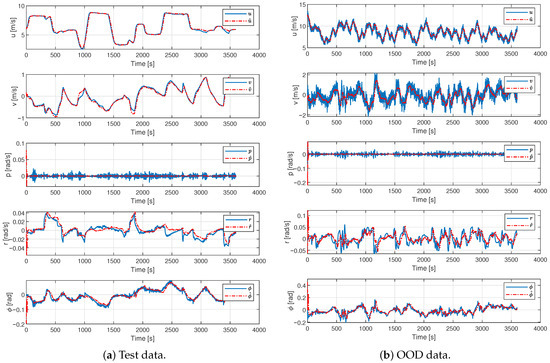
Figure 9.
State-space model validation.
Table 7 highlight the strong predictive performance of the state-space formulation. For u, v, and , the NMSE values remained consistently low in the test, validation, and out-of-distribution datasets, demonstrating both accuracy and generalization. Notably, the state-space model achieved the best overall balance among the four methods tested, with NMSE values as low as 0.0246 for u under test conditions and 0.0499 under OOD conditions. The time series comparisons further show that the model accurately reproduces both the amplitude and phase of vessel responses, underscoring its robustness in capturing essential oscillatory and transient behaviors.
Table 7.
NMSE state-space model results.
In addition, the residual statistics summarized in Table 8 show that the state-space model produces unbiased errors across all datasets, with residual means consistently close to zero for the five output variables. The standard deviations remain small across the Train, Test, and Validation partitions, indicating that the model accurately captures the distribution of the training data. The increase in residual variance observed in the OOD dataset is expected, since these trajectories contain maneuvering conditions not present during identification. Notably, the angular variables , , and exhibit extremely small residual means (–) and low dispersion, confirming that the short-term rotational dynamics are well represented by the identified model. Overall, the results indicate that the state-space representation is unbiased and stable, and that its prediction errors can be interpreted as noise rather than structural model deficiencies.
Table 8.
Residuals mean ± standard deviation for the state space model.
Beyond predictive accuracy, the state-space formulation provides a flexible structure that can be adapted to different experimental frameworks. By modifying the input and output matrices, the model can be extended to incorporate additional environmental effects, alternative propulsion systems, or sensor configurations. This scalability makes the state-space model a valuable foundation for future experimentation, allowing researchers to simulate a variety of maneuvering conditions and to design advanced predictive controllers grounded in realistic vessel dynamics.
6.5. Temporal Stability Analysis
To evaluate temporal stability, the models were assessed using four prediction horizons: 1-step, 5-step, 15-step, and 30-step. For each horizon h, the regression models and the state-space model were evaluated against shifted targets , without modifying the internal structure of the models (Table 9).
Table 9.
NMSE for multi-step prediction horizons (1, 5, 15, 30 steps) under OOD evaluation.
Across all models, the multi-step results reveal a consistent degradation in accuracy as the prediction horizon increases, which is expected in dynamical systems where errors propagate through time. Both linear and polynomial regression exhibit a gradual increase in NMSE for u, v, r, and , while maintaining an almost constant error for p, indicating that roll-rate dynamics are simpler and less prone to temporal drift. In contrast, the state-space model demonstrates the best short-horizon performance (1–5 steps), particularly for u and , but its advantage diminishes at longer horizons, where all models converge toward similar error magnitudes. Notably, the NMSE at the 15-step horizon remains within the monotonic trend of intermediate degradation observed between 5 and 30 steps, confirming that constitutes a representative mid-range horizon where temporal stability can be evaluated without reaching the saturation error region observed at 30 steps.
6.6. Statistical Significance
Statistical confidence measures of the performance metrics were employed to quantify the variability and statistical reliability of the NMSE across all datasets used in this work. For this purpose, a bootstrap-based analysis with 100 iterations was conducted.
In each bootstrap iteration, a new model was trained using a resampled version of the training data, while the NMSE was computed independently for the four evaluation datasets. Table 10 and Table 11 report the mean ± one standard deviation of the NMSE over the 100 iterations for all modeling approaches considered in this work.
Table 10.
NMSE mean ± standard deviation for the linear regression model.
Table 11.
NMSE mean ± standard deviation for the third-order polynomial regression model.
This bootstrap procedure serves two main purposes:
- To quantify the sensitivity of each model to sampling variability, that is, the stability of its parameters within the training distribution.
- To reveal the growth of epistemic uncertainty during extrapolation toward previously unseen extreme operating conditions (distribution shift).
Table 10 and Table 11 present the results corresponding to the regression-based models. These models exhibit extremely small standard deviations across all datasets (on the order of –), indicating that both the linear and polynomial models display a highly stable behavior under resampling of the training set. This result suggests that the models are not overly sensitive to fluctuations in the training data and that their predictive performance remains consistent across repeated training instances.
7. Conclusions and Future Research Lines
This study developed and evaluated four interpretable models—linear regression, third-order polynomial regression, state-space, and ARX—to predict the maneuverability of a river patrol vessel in 4-DoF: u, v, , and r. By incorporating roll dynamics into the modeling framework, the research addressed a limitation of conventional 3-DoF approaches and provided a more comprehensive representation of vessel behavior under realistic operating conditions.
Comparative analysis demonstrated that all models successfully captured the main dynamics of the vessel, achieving low NMSE values across the training, validation, and OOD datasets. The state-space model yielded the best overall performance, with NMSE as low as 0.0246 for u under test conditions and 0.0499 for the OOD scenarios, confirming its strong generalizability. The ARX model showed robust performance, achieving the lowest NMSE for u in the test dataset (0.0149) and maintaining stability under OOD conditions, although its accuracy decreased for dynamics v and r. Regression-based models, while less precise, provided transparent formulations with acceptable error levels (e.g., NMSE < 0.10 across most variables), which makes them suitable for real-time monitoring and control prototyping.
From a scientific perspective, these findings confirm the value of interpretable system identification approaches in ship maneuverability. Regression models offer computational efficiency and simplicity, the ARX model highlights the advantages of temporal dependence for forecasting, and the state-space formulation provides a scalable framework for reconstructing internal dynamics and extending the model to more complex experimental conditions. The inclusion of OOD testing further underscores the robustness of the proposed methodologies, demonstrating their applicability in scenarios beyond the training distribution, which is critical for real-world deployment.
A principal limitation of this study is that all models were developed and evaluated exclusively using simulated data generated from a validated 4-DoF maneuvering environment. Although this approach facilitates controlled experimentation, ensures reproducibility, and allows systematic assessment of model performance under routine and extreme (OOD) operating conditions, it does not capture sensor noise, environmental uncertainty, unmodeled hydrodynamics, or operational factors present in real ship trials. As such, empirical validation with full-scale maneuvering data is a necessary next step to assess the robustness and practical reliability of the identified models. Future work will therefore focus on deploying the state-space and ARX formulations on an operational vessel to evaluate their behavior under real-world disturbances and measurement imperfections, enabling refinement and calibration of the models toward field-ready performance.
A second limitation of the present study is that the computational performance of the identified models was not evaluated on a real hardware platform. Although the mathematical formulations used—particularly the ARX and state-space models—are well suited for embedded execution due to their low computational complexity, the manuscript focuses exclusively on offline prediction. As a result, execution times, memory requirements, and real-time stability on embedded marine controllers were not assessed. Future work will therefore include hardware-in-the-loop experiments and benchmarking on representative embedded systems (e.g., ARM-based processors or industrial marine microcomputers) to ensure that the models meet real-time constraints required for onboard navigation and control applications.
A further limitation concerns the absence of maneuverability indices commonly used in naval architecture, such as turning diameter, tactical diameter, advance, transfer, or yaw response time—to assess ship handling performance. These metrics require structured, repeatable control protocols (e.g., IMO-standard turning-circle or zigzag maneuvers), which are not present in the randomly generated excitation sequences that compose the current simulation dataset. For this reason, such indices could not be computed in the present study. Future work will incorporate simulated and full-scale trials specifically designed to reproduce standardized maneuvers, enabling a comprehensive comparison between model predictions and accepted hydrodynamic performance criteria.
In general, this work establishes a foundation for integrating interpretable machine learning with classical system identification to design predictive controllers, autonomous navigation strategies, and combat training simulations in riverine environments. Future research may extend the state-space formulation to hybrid or nonlinear structures, integrate additional environmental disturbances such as currents and shallow-water effects, and validate the models using full-scale experimental data to further enhance their operational reliability.
Future research lines derived from this work may follow several directions. First, extending the current framework to hybrid or nonlinear state-space models would enable integrating hydrodynamic theory with data-driven corrections, thereby improving accuracy while preserving interpretability in complex maneuvering conditions. Second, incorporating additional environmental disturbances, such as river currents, shallow-water effects, and varying payloads, would increase the robustness and realism of the models, enabling more reliable predictions across diverse operating scenarios. Finally, validation through full-scale experimental trials with patrol vessels is essential to confirm the applicability of the proposed models in real-world conditions, providing empirical evidence to refine predictive controllers and autonomous navigation strategies.
Another promising line of research is the generalization of the developed models to motion platforms with varying DoF. By adapting the state-space and ARX formulations, the methodology can be scaled beyond the 4-DoF representation of the patrol vessel to higher-DoF systems, such as 5-DoF or 6-DoF marine vehicles, or even to terrestrial and aerial platforms. This scalability would allow the framework to serve as a unifying approach for modeling and predicting the dynamics of diverse maneuvering systems, thereby broadening its applicability across experimental testbeds, training simulators, and autonomous vehicle design in different domains.
Author Contributions
Conceptualization, J.C.M. and J.E.-G.; Methodology, J.C.M. and J.E.-G.; Software, D.O.-B., K.V.G., C.S.M. and R.S.-D.; Validation, A.L.A., C.S.M., R.S.-D., J.J.-C. and J.E.-G.; Formal analysis, J.C.M. and J.O.L.; Investigation, J.C.M., C.S.M., J.J.-C. and J.E.-G.; Data curation, D.O.-B., K.V.G., J.J.-C. and J.O.L.; Writing—original draft preparation, J.C.M., D.O.-B. and K.V.G.; Writing—review and editing, A.L.A. and J.E.-G.; Visualization, K.V.G. and J.O.L.; Supervision, J.E.-G.; Project administration, A.L.A.; Funding acquisition, A.L.A. and R.S.-D. All authors have read and agreed to the published version of the manuscript.
Funding
This work was possible thanks to financing from the Ministry of Science, Technology, and Innovation of Colombia—Minciencias, within the framework agreement for collaboration N° 877-2017 for the development project N° 1126-1022-82866. We also thank the “Almirante Padilla” Naval School—ENAP, Marine Infantry Training Center. School—EFIM, and to the International Center of Advanced Fluvial Excellence—CIEAF, for their valuable assistance in carrying out the online surveys that contributed to the development of this research.
Data Availability Statement
The original contributions presented in this study are included in the article. Further inquiries can be directed to the corresponding authors.
Conflicts of Interest
Author Carlos Soto Montaño and José Oñate López were employed by the company ONIRIS ID SAS. The remaining authors declare that the research was conducted in the absence of any commercial or financial relationships that could be construed as a potential conflict of interest.
References
- Lan, J.; Zheng, M.; Chu, X.; Ding, S. Parameter Prediction of the Non-Linear Nomoto Model for Different Ship Loading Conditions Using Support Vector Regression. J. Mar. Sci. Eng. 2023, 11, 903. [Google Scholar] [CrossRef]
- Abkowitz, M. Measurement of hydrodynamic characteristics from ship maneuvering trials by system identification. Trans. Soc. Nav. Archit. Mar. Eng. 1980, 88, 283–318. [Google Scholar]
- Yasukawa, H.; Yoshimura, Y. Introduction of MMG standard method for ship maneuvering predictions. J. Mar. Sci. Technol. 2015, 20, 37–52. [Google Scholar] [CrossRef]
- Moreno-Salinas, D.; Chaos, D.; De la Cruz, J.; Aranda, J. Identification of a Surface Marine Vessel Using LS-SVM. J. Appl. Math. 2013, 2013, 803548. [Google Scholar] [CrossRef]
- Carrillo, S.; Contreras, J. Obtaining First and Second Order Nomoto Models of a Fluvial Support Patrol using Identification Techniques. Cienc. Tecnol. Buques 2018, 11, 19–28. [Google Scholar] [CrossRef]
- Zhang, X.; Zhao, B.; Zhang, G. Improved parameter identification algorithm for ship model based on nonlinear innovation decorated by sigmoid function. Transp. Saf. Environ. 2021, 3, 114–122. [Google Scholar] [CrossRef]
- Fukui, Y.; Yokota, H.; Yano, H.; Kondo, M.; Nakano, T.; Yoshimura, Y. 4-DOF Mathematical Model for Manoeuvring Simulation including Roll Motion. J. Jpn. Soc. Nav. Archit. Ocean Eng. 2016, 24, 167–179. [Google Scholar] [CrossRef][Green Version]
- Zhao, B.; Zhang, X.; Liang, C. A Novel Parameter Identification Algorithm for 3-DOF Ship Maneuvering Modelling Using Nonlinear Multi-Innovation. J. Mar. Sci. Eng. 2022, 10, 581. [Google Scholar] [CrossRef]
- Yu, Q.; Yang, Y.; Geng, X.; Jiang, Y.; Li, Y.; Tang, Y. Integrating Computational Fluid Dynamics for Maneuverability Prediction in Dual Full Rotary Propulsion Ships: A 4-DOF Mathematical Model Approach. J. Mar. Sci. Eng. 2024, 12, 762. [Google Scholar] [CrossRef]
- Tillig, F.; Ringsberg, J. A 4 DOF simulation model developed for fuel consumption prediction of ships at sea. Ships Offshore Struct. 2018, 14, 112–120. [Google Scholar] [CrossRef]
- Zhang, C.; Liu, X.; Wan, D.; Wang, J. Experimental and numerical investigations of advancing speed effects on hydrodynamic derivatives in MMG model, Part I: Xvv, Yv, Nv. Ocean Eng. 2019, 179, 67–75. [Google Scholar] [CrossRef]
- Meng, Y.; Zhang, X.; Zhu, J. Parameter identification of ship motion mathematical model based on full-scale trial data. Int. J. Nav. Archit. Ocean Eng. 2022, 14, 100437. [Google Scholar] [CrossRef]
- Escorcia-Gutierrez, J.; Gamarra, M.; Beleño, K.; Soto, C.; Mansour, R.F. Intelligent deep learning-enabled autonomous small ship detection and classification model. Comput. Electr. Eng. 2022, 100, 107871. [Google Scholar] [CrossRef]
- Zhu, Z.; Kim, B.S.; Wang, S.; Kim, Y. Study on numerical PMM test and its application to KCS hull. Appl. Ocean Res. 2022, 127, 103327. [Google Scholar] [CrossRef]
- Hu, Y.; Song, L.; Liu, Z.; Yao, J. Identification of Ship Hydrodynamic Derivatives Based on LS-SVM with Wavelet Threshold Denoising. J. Mar. Sci. Eng. 2021, 9, 1356. [Google Scholar] [CrossRef]
- Jeon, M.; Yoon, H.; Park, J.; Rhee, S.; Seo, J. Identification of 4-DoF maneuvering mathematical models for a combatant in intact and damaged conditions. Int. J. Nav. Archit. Ocean Eng. 2022, 14, 100480. [Google Scholar] [CrossRef]
- Song, L.; Hao, L.; Tao, H.; Xu, C.; Guo, R.; Li, Y.; Yao, J. Research on Black-Box Modeling Prediction of USV Maneuvering Based on SSA-WLS-SVM. J. Mar. Sci. Eng. 2023, 11, 324. [Google Scholar] [CrossRef]
- Chattha, N.; Siddiqui, S.; Malik, M.; Elst, L.; Dengel, A.; Ahmed, S. KINN: Incorporating Expert Knowledge in Neural Networks. arXiv 2019, arXiv:1902.05653. [Google Scholar] [CrossRef]
- Wu, T.; Li, R.; Chen, Q.; Pi, G.; Wan, S.; Liu, Q. A Numerical Study on Modeling Ship Maneuvering Performance Using Twin Azimuth Thrusters. J. Mar. Sci. Eng. 2023, 11, 2167. [Google Scholar] [CrossRef]
- Alexandersson, M.; Mao, W.; Ringsberg, J. System identification of Vessel Manoeuvring Models. Ocean Eng. 2022, 266, 112940. [Google Scholar] [CrossRef]
- Liu, Y.; Xue, Y.; Huang, S.; Xue, G.; Jing, Q. Dynamic Model Identification of Ships and Wave Energy Converters Based on Semi-Conjugate Linear Regression and Noisy Input Gaussian Process. J. Mar. Sci. Eng. 2021, 9, 194. [Google Scholar] [CrossRef]
- Baier, A.; Aspandi, D.; Staab, S. ReLiNet: Stable and Explainable Multistep Prediction with Recurrent Linear Parameter Varying Networks. In Proceedings of the Thirty-Second International Joint Conference on Artificial Intelligence (IJCAI-23), Macao, China, 19–25 August 2023; pp. 3461–3469. [Google Scholar] [CrossRef]
- Miller, A. Ship Model Identification with Genetic Algorithm Tuning. Appl. Sci. 2021, 11, 5504. [Google Scholar] [CrossRef]
- Baier, A.; Staab, S. A Simulated 4-DOF Ship Motion Dataset for System Identification under Environmental Disturbances; DaRUS: Sttutgart, Germany, 2022. [Google Scholar] [CrossRef]
- Isherwood, R. Wind resistance of merchant ships. Trans. RINA 1973, 115, 327–338. [Google Scholar]
- Hasselmann, K.; Barnett, T.P.; Bouws, E.; Carlson, H.; Cartwright, D.E.; Enke, K.; Ewing, J.; Gienapp, A.; Hasselmann, D.; Kruseman, P.; et al. Measurements of wind-wave growth and swell decay during the Joint North Sea Wave Project (JONSWAP). Ergaenzungsheft Dtsch. Hydrogr. Z. Reihe A 1973, 12, 1–95. [Google Scholar]
- Frank, D.; Aspandi, D.; Muehlebach, M.; Unger, B.; Staab, S. Robust Recurrent Neural Network to Identify Ship Motion in Open Water with Performance Guarantees—Technical Report. arXiv 2022, arXiv:2212.05781. [Google Scholar]
- De Moor, B.; Van Overschee, P.; Favoreel, W. Algorithms for subspace state-space system identification: An overview. In Applied and Computational Control, Signals, and Circuits: Volume 1; Springer: Berlin/Heidelberg, Germany, 1999; pp. 247–311. [Google Scholar]


Disclaimer/Publisher’s Note: The statements, opinions and data contained in all publications are solely those of the individual author(s) and contributor(s) and not of MDPI and/or the editor(s). MDPI and/or the editor(s) disclaim responsibility for any injury to people or property resulting from any ideas, methods, instructions or products referred to in the content. |
© 2025 by the authors. Licensee MDPI, Basel, Switzerland. This article is an open access article distributed under the terms and conditions of the Creative Commons Attribution (CC BY) license (https://creativecommons.org/licenses/by/4.0/).