An Improved Physics-Informed Neural Network Approach for Solving the FitzHugh–Nagumo Equation

Abstract

The FitzHugh–Nagumo (FHN) equation in one dimension is solved in this paper using an improved physics-informed neural network (PINN) approach. Examining test problems with known analytical solutions and the explicit finite difference method (EFDM) allowed for the demonstration of the PINN’s effectiveness. Our study presents an improved PINN formulation tailored to the FitzHugh–Nagumo reaction–diffusion system. The proposed framework is efficiently designed, validated, and systematically optimized, demonstrating that a careful balance among model complexity, collocation density, and training strategy enables high accuracy within limited computational time. Despite the very strong agreement that both methods provide, we have demonstrated that the PINN results exhibit a closer agreement with the analytical solutions for Test Problem 1, whereas the EFDM yielded more accurate results for Test Problem 2. This study is crucial for evaluating the PINN’s performance in solving the FHN equation and its application to nonlinear processes like pulse propagation in optical fibers, drug delivery, neural behavior, geophysical fluid dynamics, and long-wave propagation in oceans, highlighting the potential of PINNs for complex systems. Numerical models for this class of nonlinear partial differential equations (PDEs) may be developed by existing and future model creators of a wide range of various nonlinear physical processes in the physical and engineering sectors using the concepts of the solution methods employed in this study.

1. Introduction

Analytical techniques and numerical simulations of nonlinear partial differential equations (PDEs) have been extensively studied across various fields, including mathematics, physics, chemistry, and engineering. The complexity of nonlinear PDEs continues to grow as more real-world factors influencing engineering systems are incorporated. Among these, the FitzHugh–Nagumo (FHN) equation plays a crucial role. It is widely used in the study of diverse engineering problems, fiber optics, and neurophysiology [1]. The FHN model effectively describes phenomena such as solitary pulses and periodic wave trains in systems like photonic crystals, semiconductors, and fiber optic communication networks [2]. Since analytical solutions for the FHN equation are rare, there is intensive research on numerical methods. Thus, a variety of numerical methods have been applied to solve the FHN equation, including the Haar-scale-3 wavelet collocation method [3], Rabotnov’s fractional exponential function approach [4], the two-step hybrid block method [5], the local meshless method [6], the Chebyshev polynomial-based collocation method [7], the compact finite difference method [8], the spectral Galerkin method [9], semi-analytical methods [10], the cubic B-spline-based one-step optimal hybrid block method [11], the fully discrete implicit-explicit finite element method [12], and the sixth-order compact finite difference method [13].

One should note that the classical FHN model consists of two coupled fields: an activator, which evolves rapidly and includes a cubic nonlinear reaction term, and an inhibitor (recovery variable), which evolves on a slower timescale and provides negative feedback. The one-field PDE with a cubic reaction term, which we solve in this work, corresponds to the fast subsystem of the FHN model, obtained by assuming that the inhibitor variable equilibrates instantaneously (i.e., adiabatic or singular perturbation limit). Mathematically, this corresponds to taking the limit where the inhibitor relaxation time tends to zero, so that the inhibitor variable can be expressed algebraically as a function of the activator and eliminated. This reduction is valid in the regime where (i) timescale separation is extreme, and the inhibitor recovers much faster than the activator evolves, (ii) spatial coupling of the inhibitor is negligible, or its diffusion is either vanishingly small or homogenized, and (iii) the dominant dynamics of interest arise from wave propagation shaped primarily by the cubic reaction term. This reduced model is therefore appropriate for studying front propagation, bistability, and excitable pulse initiation in regimes where recovery is effectively instantaneous. By eliminating the inhibitor variable, the features of the full FHN system, such as slow recovery dynamics, inhibitor diffusion, relaxation oscillations, and spike frequency adaptation, are no longer captured.

Most traditional numerical methods for solving PDEs rely on discretizing the problem domain using a mesh (or grid) of finite points. This approach requires the problem to be formulated in terms of discrete spatial and temporal variables. While such mesh-based techniques are widely used and considered effective in many scenarios, they face significant challenges when applied to high-dimensional problems. As the number of dimensions increases, the mesh must become increasingly refined, which leads to an exponential growth in the number of grid points. This, in turn, results in a sharp increase in computational complexity, as the algorithm requires more processing power and memory to handle the larger grid. This high-dimensional scaling problem becomes especially pronounced in fields like fluid dynamics, material science, and complex biological systems, where the number of variables and their interactions can be vast. In response to these limitations, a new class of modeling approaches has emerged, driven by advancements in artificial intelligence and computational power. One such technique, PINNs, represents a significant departure from traditional mesh-based methods. Unlike conventional approaches, PINNs leverage neural networks to learn the solution to a PDE directly from the governing equations and data, without the need for a predefined mesh. By incorporating physical laws into the loss function of the neural network, PINNs can efficiently solve complex nonlinear PDEs, even in high-dimensional spaces, without suffering from the computational burdens associated with grid refinement. Recent work by Raissi et al. [14] has highlighted the power and versatility of PINNs in solving a range of challenging nonlinear PDEs. Their research demonstrated that PINNs can effectively tackle problems such as nonlinear Schrödinger equations, Allen–Cahn equations, Navier–Stokes equations, Korteweg–de Vries equations, and Burgers’ equation. Furthermore, they have proven to be a valuable tool for addressing high-dimensional inverse problems, where traditional methods often struggle with scalability and efficiency. These developments mark a promising shift towards more flexible and scalable techniques for solving complex, real-world problems across various scientific disciplines.

In this study, we compare an improved PINN approach with the standard EFDM to solve the FHN equation. The FDM approximates derivatives at discrete points by constructing a grid and calculating differences between nearby values, with accuracy depending on grid step size and derivative approximation order. In contrast, PINN is a machine learning-based method where a neural network is trained to minimize the residual between the predicted and actual solution, effectively handling complex boundary conditions and geometries. However, PINNs can be computationally expensive and sensitive to hyperparameters like network architecture.

Although promising, PINN’s accuracy compared to conventional methods like FDM still remains largely unexplored. In our previous work, EFDM outperformed PINN in solving the Burgers’ and Sine-Gordon equations [15,16]. To make further progress in this regard, in this work, we present the first comparison, to the best of our knowledge, of EFDM and improved PINN for solving the FHN equation, using two test problems with different initial and boundary conditions. This contrasts with other studies focused primarily on comparison between conventional numerical methods, like explicit and implicit time-stepping methods for the FHN equation [17].

2. The FitzHugh–Nagumo Equation

We considered the FHN equation, which is a nonlinear PDE given by [8]

$$\begin{gathered} {\displaystyle \frac{\partial u\left(x,t\right)}{\partial t}}=\alpha \left(t\right){\displaystyle \frac{{\partial }^{2}u\left(x,t\right)}{\partial x^2}}+\beta \left(t\right){\displaystyle \frac{\partial u\left(x,t\right)}{\partial x}}\gamma \left(t\right)u\left(x,t\right)\left(u\left(x,t\right)-\mu \right)\left(1-u\left(x,t\right)\right), \\ a\le x\le b, 0\le t\le T \end{gathered}$$

(1a)

We note that in Equation (1a), α(t) multiplies the second spatial derivative (diffusion term), whereas β(t) multiplies the first spatial derivative (advection term). In the case of $\alpha \left(t\right)=1, \beta \left(t\right)=0, \gamma \left(t\right)=1, \mathrm{E}\mathrm{q}\mathrm{u}\mathrm{a}\mathrm{t}\mathrm{i}\mathrm{o}\mathrm{n} \left(1\mathrm{a}\right) \mathrm{b}\mathrm{e}\mathrm{c}\mathrm{o}\mathrm{m}\mathrm{e}\mathrm{s}$ [11]:

$$\begin{gathered} {\displaystyle \frac{\partial u\left(x,t\right)}{\partial t}}={\displaystyle \frac{{\partial }^{2}u\left(x,t\right)}{\partial x^2}}+u\left(x,t\right)\left(u\left(x,t\right)-\mu \right)\left(1-u\left(x,t\right)\right), \\ a\le x\le b, 0\le t\le T \end{gathered}$$

(1b)

The initial condition for Equation (1a,b) is given as follows:

$$u\left(x,t=0\right)=u_0\left(x\right), a\le x\le b$$

(2)

and boundary conditions read as

$$u\left(x=a,t\right)=u_a\left(t\right), u\left(x=b,t\right)=u_b\left(t\right), 0<t\le T$$

(3)

where μ is the positive parameter and t and x are space and time variables, respectively.

3. Explicit Finite Difference Method

Using the EFDM, where the forward FD scheme is used to represent the derivative term $\partial u(x,t)/\partial t=\left(u_i^{j+1}-u_i^j\right)/∆t$ and central FD schemes are used to represent derivative terms $\left(\partial u(x,t)/\partial x\right)$ = $(u_{i+1}^j-u_{i-1}^j)/2\Delta x$ and $\partial u(x,t)/\partial x=\left(u_{i+1}^j-{2u_i^j+u}_{i-1}^j\right)/{\left(∆x\right)}^2$, Equation (1a) is written in the following form:

$${\displaystyle \frac{u_i^{j+1}-u_i^j}{∆t}}=\alpha \left(t_j\right){\displaystyle \frac{u_{i+1}^j-{{2u}_i^j+u}_{i-1}^j}{{\left(∆x\right)}^2}}+\beta \left(t_j\right){\displaystyle \frac{u_{i+1}^j-u_{i-1}^j}{2∆x}}+\gamma \left(t_j\right)\left({\left(u_i^j\right)}^3-{\left(u_i^j\right)}^2\left(1+\mu \right)+{\mu u}_i^j\right)$$

(4a)

and Equation (1b) is given as follows:

$${\displaystyle \frac{u_i^{j+1}-u_i^j}{∆t}}={\displaystyle \frac{u_{i+1}^j-{{2u}_i^j+u}_{i-1}^j}{{(∆x)}^2}}-{\left(u_i^j\right)}^3+{\left(u_i^j\right)}^2\left(1+\mu \right)-{\mu u}_i^j$$

(4b)

where $u_i^j\equiv u(x_i,t_j)$, and indexes i and j refer to the discrete step lengths $\Delta$x and $\Delta$t for the coordinate x and time t. The grid dimensions in the x and t directions are $K=1/\Delta x$ and $M=T/\Delta t$, respectively. Using the FD scheme, the initial condition (2) and boundary conditions (3) are given as follows:

$$u_i^1=u_0\left(x_i\right), a\le x_i\le b, i=1, 2,\dots ,K (t=0)$$

(5)

$$u_1^j=u_a\left(t_j\right), u_K^j=u_b\left(t_j\right), j=1, 2,\dots ,M (x=a \mathrm{a}\mathrm{n}\mathrm{d} x=b)$$

(6)

Equation (4b) represents a formula for $u_i^{j+1}$ at the (i, j+1)th mesh point in terms of the known values along the jth time row. The truncation error can be reduced using small enough values of $\Delta$t and $\Delta$x until the precision attained is within the error tolerance.

4. Physics-Informed Neural Networks

4.1. The Basic Concept of the PINNs Is Solving PDEs

A machine learning method called the PINN can be used to approximately solve PDEs. A general form of PDEs with corresponding initial and boundary conditions is

$$\begin{array}{l}{\displaystyle \frac{\partial u(x,t)}{\partial t}}+{\rm N}\left[u(x,t)\right]=0,\hspace{0.17em}\hspace{0.17em}\hspace{0.17em}\hspace{0.17em}\hspace{0.17em}x\in \Omega ,\hspace{0.17em}\hspace{0.17em}\hspace{0.17em}\hspace{0.17em}t\in [0,T]\\ u(x,t=0)=h(x),\hspace{0.17em}\hspace{0.17em}\hspace{0.17em}x\in \Omega \\ u(x,t)=g(x,t),\hspace{0.17em}\hspace{0.17em}\hspace{0.17em}x\in {\Omega }_g,\hspace{0.17em}\hspace{0.17em}\hspace{0.17em}\hspace{0.17em}t\in [0,T]\hspace{0.17em}\end{array}$$

(7)

Here, N is a differential operator, $x\in \Omega \subseteq R^d$ and $t\in R$ represent spatial and temporal dimensions, respectively, $\Omega \subseteq R^d$ is a computational domain, ${\Omega }_g\subseteq \Omega$ is a computational domain of the exposed boundary conditions, and $u(x,t)$ is the solution of the PDEs with the initial condition $h(x)$ and boundary conditions $g(x,t)$.

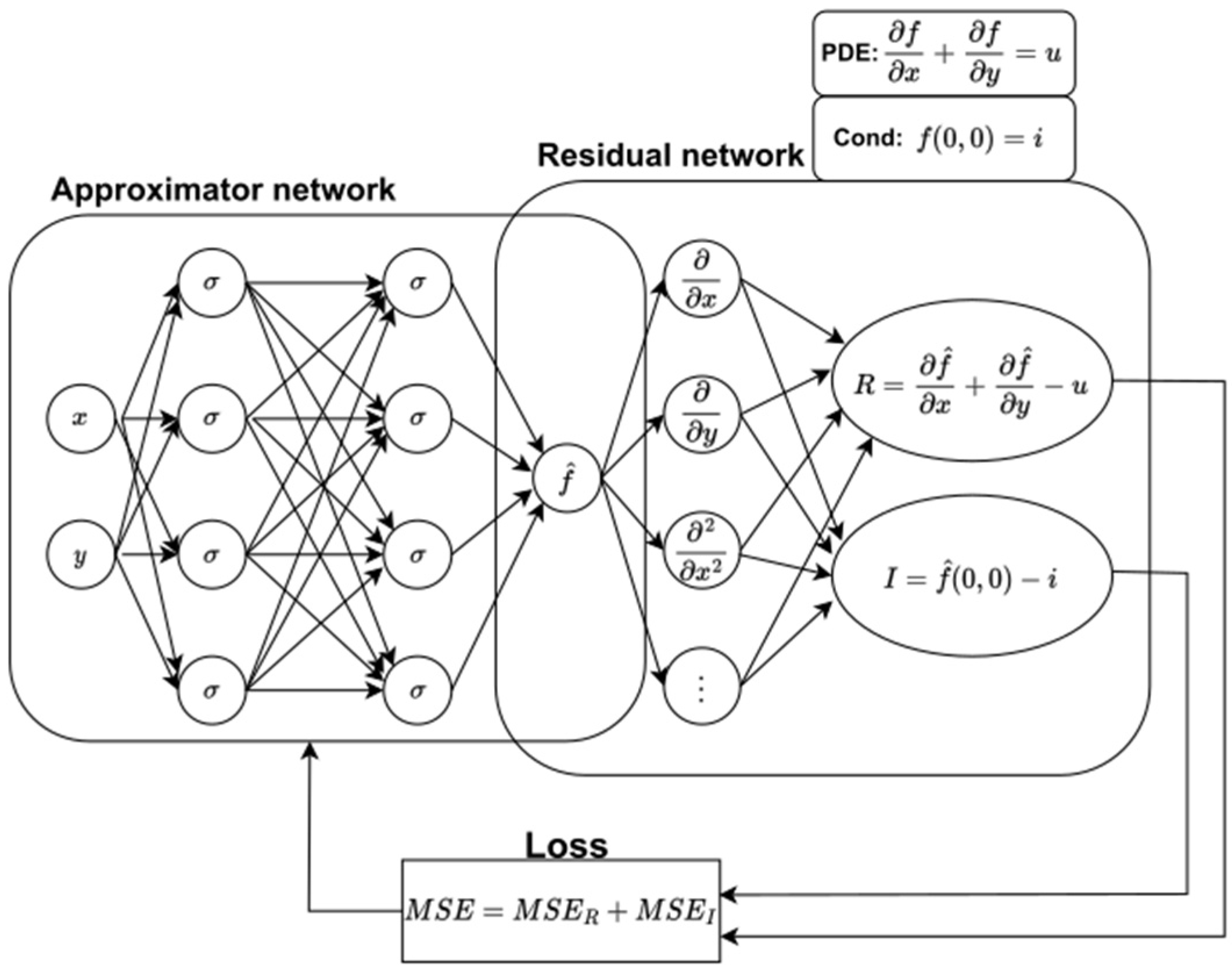
The approximator network and the residual network are the two subnets that make up PINN in its original construction [18]. The approximator network receives input $(x,t)$, undergoes the training process, and provides an approximate solution $\stackrel{⌢}{u}(x,t)$ as an output. The approximator network is trained using a grid of collocation points, which are sampled randomly or regularly from the simulation domain. To optimize the network’s weights and biases, a composite loss function is minimized:

$$L=L_r+L_0+L_b$$

(8)

where

$$\begin{gathered} L_r={\displaystyle \frac{1}{N_r}}{{\displaystyle \sum _{i=1}^{N_r}\left|u(x^i,t^i)+N[u(x^i,t^i)]\right|}}^2 \\ L_0={\displaystyle \frac{1}{N_0}}{{\displaystyle \sum _{i=1}^{N_0}\left|u(x^i,t^i)-h^i)]\right|}}^2 \\ L_b={\displaystyle \frac{1}{Nb}}{{\displaystyle \sum _{i=1}^{N_b}\left|u(x^i,t^i)-g^i)]\right|}}^2 \end{gathered}$$

(9)

Here, $L_r$, $L_0$, and $L_b$ represent residuals of governing equations and initial and boundary conditions, respectively. $N_r$, $N_0$, and $N$ are the numbers of mentioned collocation points of the computational domain and initial and boundary conditions, respectively. The residuals are computed by the residual network, a non-trainable component of the PINN model. To calculate these residuals, PINN requires derivatives of the outputs with respect to inputs x and t. Automated differentiation (AD) is used to compute these derivatives by integrating the derivatives of individual operations, which is a key feature distinguishing PINNs from earlier methods that relied on manually derived back-propagation rules. Only first- and second-order spatial derivatives appear in the residual. Automatic differentiation computes these exactly and directly. No hidden higher-order derivatives or regularization terms are introduced through the AD graph. The script can be checked at GitHub Repository. Deep learning frameworks like TensorFlow 2.13.0 and PyTorch 2.1.0 provide robust AD, enabling efficient calculation of derivatives of all orders in space–time without the need for manual derivation or numerical discretization. We use default unity weights for loss components for the PDE itself, as well as boundary and initial conditions. To check the impact of various weight distributions on the result, we checked three different weight distributions, with each of them putting emphasis on the PDE, boundary condition (BC), and initial condition (IC). The findings show that, for this specific problem, there is no statistically significant impact, bearing in mind the variance introduced by different seeds.

A schematic of the PINN is demonstrated in Figure 1, in which a simple PDE $\partial f/\partial x+\partial f/\partial y=u$ is used as an example. The approximator network is used to approximate the solution $u(x,t)$, which then goes to the residual network to calculate the residual loss $L_r$, boundary condition loss $L_b$, and initial condition loss $L_0$. The weights and biases of the approximator network are trained using a composite loss function consisting of residuals $L_r$, $L_0$, and $L_b$ through the gradient-descent technique based on the back-propagation. For a simple PDE shown at the top of Figure 1, the residuals are defined as $\mathrm{R}=\partial \stackrel{⌢}{f}/\partial x+\partial \stackrel{⌢}{f}/\partial y-u$ and $\mathrm{I}=\stackrel{⌢}{f}(0,0)-i$. The total loss function combines the mean squared errors of these two terms, ensuring both the PDE and its conditions are satisfied: MSE = MSE_R + MSE_I, where MSE_R represents the mean squared residual of the PDE and MSE_I enforces the initial or boundary conditions. During training, the network parameters are optimized to minimize this combined loss, leading to a solution that simultaneously approximates f(x, y) and adheres to the underlying physical constraints. This approach enables the PINN to solve PDEs in a mesh-free manner while integrating physical laws directly into the learning process, making it highly effective for modeling complex systems in fluid dynamics, heat transfer, and other physics-based domains.

It is also interesting to note that a previous research study focused on the synthesis of a four-bar mechanism for the trajectory planning of a point belonging to the connecting rod [19]. The objective was to generate a tool that synthesizes the mechanism topology given the desired trajectory. This preliminary study has shown how PINNs are suitable to automate the synthesis of mechanisms, where regular NNs would generally fail. Numerical analyses also demonstrate that a PINN learns relations from a physical numerical model in a more efficient way than a traditional NN.

4.2. Implementation of PINN in Solving the FitzHugh–Nagumo Equation

We used the DeepXDE 1.14.0 library to construct the PINN model for solving the FHN equation [20]. Our PINN has two inputs (x, t) and three layers, and each layer has 30 neurons. All neurons use a Tanh activation function. The collocation points are divided into three subsets: the largest (8000 points) covers the problem domain, while the second and third subsets (400 and 800 points) impose boundary and initial conditions. Both test cases share the same conditions. The PINN training consists of two phases: in the first, weights and biases are optimized using the Adam algorithm with a learning rate of 10⁻³. In the second phase, the Limited Memory Broyden–Fletcher–Goldfarb–Shanno (L-BFGS) algorithm is used to refine the solution after the “global” search phase, as described in [21]. The entire training process takes about 85 s on the NVIDIA Tesla T4 GPU. Due to lost implementation details, we approximated the training as follows: Adam was run for ~40,000 epochs until the loss stabilized, followed by L-BFGS for ~200 iterations, with early stopping criteria activated. The stopping criterion was defined as either the loss dropping below 1 × 10⁻⁸ or minimal change between iterations. Sample points were chosen using uniform random sampling in the domain. The assumed boundary and initial conditions are given in Equation (7).

While different hyperparameters, activation functions, training methods, and PINN topologies could yield better solutions, we chose the most common values from the FHN literature, as hyperparameter tuning is a time-consuming process beyond the scope of this work. We conducted a brief hyperparameter analysis, changing one kind of hyperparameter at a time and monitoring the change in RMSE:

• Various activation functions: tanh—0.000039; swish—0.000040; sin—0.000035; sigmoid—0.000070.
• Various PINN architectures (layers × neurons per layer): 3 × 10—0.000046; 3 × 30—0.000039; 3 × 50—0.000020; 4 × 30—0.000018; 4 × 50—0.000014.
• Various numbers of collocation points (PDE, BC, IC): (2000, 100, 200)—0.000059; (4000, 200, 400)—0.000055; (8000, 400, 800)—0.000039; (16,000, 800, 1600)—0.000017.

On the other hand, RMSE variance calculated from 10 random seeds is 1.5 × 10⁻⁵, which is approximately 35% in relative RMSE terms, making the change in hyperparameters statistically insignificant. This variance justifies our choice of PINN with 3 × 30 neurons using tanh activation.

It is worth noting that the prior studies [22,23] have used hybrid neural network–metaheuristic frameworks for reliability and survival analysis. In contrast, our study introduces a PINN formulation tailored to the FHN reaction–diffusion system, with an efficient, validated, and systematically optimized PINN framework. The study achieved several key advancements in applying PINNs to the FHN system. It systematically explored hyperparameters, analyzing activation functions, network architectures, and collocation point densities, revealing that increasing both network depth and collocation density significantly improved accuracy. Despite examining larger architectures, the final model of three layers with 30 neurons struck a balance between accuracy and computational efficiency, requiring only approximately 85 s of GPU training, demonstrating that moderately sized PINNs can deliver highly accurate solutions without extensive resources. A two-stage optimization strategy combining Adam and L-BFGS enhanced convergence stability, with Adam providing global search and L-BFGS refining local minima, resulting in smoother and more precise final solutions. The robustness of the approach was verified across ten random seeds, showing a relative RMSE variance of about 35% and indicating consistent performance with low sensitivity to initialization. Comparative validation against both analytical solutions and the EFDM confirmed that the PINN accurately reproduced the expected dynamics of the FHN system. Finally, the study demonstrated that accuracy scales predictably with model complexity, as RMSE improved monotonically with increasing network depth and collocation point density, highlighting the method’s scalability and providing valuable insights for potential extensions to higher-dimensional or more complex reaction–diffusion systems.

The accuracy of the numerical results for two FHN equation test problems generated using the EFDM and PINN approach is compared to the analytical solutions presented in the literature in this research.

5. Numerical Results and Discussion

To illustrate the accuracy of the EFD scheme and PINN approach, several numerical computations are carried out for two test problems.

Test Problem 1: Consider the FHN Equation (1b) with the initial condition

$$u\left(x,t=0\right)={\displaystyle \frac{1}{2}}+{\displaystyle \frac{1}{2}}\mathrm{t}\mathrm{a}\mathrm{n}\mathrm{h}\left({\displaystyle \frac{x}{2\sqrt{2}}}\right),-10\le x\le 10$$

(10)

and boundary conditions

$$u\left(x=-10,t\right)={\displaystyle \frac{1}{2}}+{\displaystyle \frac{1}{2}}\mathrm{t}\mathrm{a}\mathrm{n}\mathrm{h}\left({\displaystyle \frac{1}{2\sqrt{2}}}(-10-{\displaystyle \frac{2\mu -1}{\sqrt{2}}}t)\right), 0<t\le T$$

(11a)

$$u\left(x=10,t\right)={\displaystyle \frac{1}{2}}+{\displaystyle \frac{1}{2}}\mathrm{t}\mathrm{a}\mathrm{n}\mathrm{h}\left({\displaystyle \frac{1}{2\sqrt{2}}}(10-{\displaystyle \frac{2\mu -1}{\sqrt{2}}}t)\right), 0<t\le T$$

(11b)

The analytical solution of the problem is given as [11]

$$u\left(x,t\right)={\displaystyle \frac{1}{2}}+{\displaystyle \frac{1}{2}}\mathrm{t}\mathrm{a}\mathrm{n}\mathrm{h}\left({\displaystyle \frac{1}{2\sqrt{2}}}(x-{\displaystyle \frac{2\mu -1}{\sqrt{2}}}t)\right)$$

(12)

Equation (12) represents a traveling-wave solution, where the hyperbolic tangent describes a wavefront moving through space over time. Such a solution is characteristic of excitable media, where a localized disturbance propagates as a pulse or wave—exactly what the FHN model captures in nerve impulse transmission or cardiac excitation.

Equation (4b) represents the EFD solution of this test problem; the initial condition (10) in terms of finite differences becomes

$$u_i^1={\displaystyle \frac{1}{2}}+{\displaystyle \frac{1}{2}}\mathrm{t}\mathrm{a}\mathrm{n}\mathrm{h}\left({\displaystyle \frac{x_i}{2\sqrt{2}}}\right), -10\le x_i\le 10, i=\mathrm{1,2},\dots ,K (t=0)$$

(13)

and boundary conditions (11) are given as

$${ u}_1^j={\displaystyle \frac{1}{2}}+{\displaystyle \frac{1}{2}}\mathrm{t}\mathrm{a}\mathrm{n}\mathrm{h}\left({\displaystyle \frac{1}{2\sqrt{2}}}(-10-{\displaystyle \frac{2\mu -1}{\sqrt{2}}}{t}_j)\right), j=\mathrm{1,2},\dots ,M (x=-10)$$

(14a)

$${ u}_K^j={\displaystyle \frac{1}{2}}+{\displaystyle \frac{1}{2}}\mathrm{t}\mathrm{a}\mathrm{n}\mathrm{h}\left({\displaystyle \frac{1}{2\sqrt{2}}}(10-{\displaystyle \frac{2\mu -1}{\sqrt{2}}}{t}_j)\right), j=\mathrm{1,2},\dots ,M (x=10)$$

(14b)

The comparison of the numerical solutions to Test Problem 1 obtained by the EFDM (step lengths are Δx = 0.5 and Δt = 0.0001) and PINN with the analytical solution (12) at different times T, by taking the parameter $\mu =0.75,$ is shown in

Table 1. Comparison of numerical and analytical solutions of Test Problem 1 for T = 0.1.

x	EFDM Solution	PINN Solution	Analytical Solution
−10	0.000828	0.000838	0.000828
−8	0.003397	0.003399	0.003396
−6	0.013827	0.013817	0.013821
−4	0.054513	0.054511	0.054504
−2	0.191626	0.191656	0.191667
0	0.493746	0.493755	0.493750
2	0.800511	0.800488	0.800467
4	0.942857	0.942839	0.942861
6	0.985476	0.985497	0.985481
8	0.996438	0.996415	0.996431
10	0.999130	0.999145	0.999130

(for T = 0.1),

Table 2. Comparison of numerical and analytical solutions of Test Problem 1 for T = 3.

x	EFDM Solution	PINN Solution	Analytical Solution
−10	0.000401	0.000417	0.000401
−8	0.001665	0.001649	0.001648
−6	0.006785	0.006738	0.006743
−4	0.027184	0.027160	0.027167
−2	0.102729	0.102986	0.103029
0	0.320470	0.320800	0.320865
2	0.660992	0.660171	0.660252
4	0.889034	0.888762	0.888809
6	0.970307	0.970474	0.970483
8	0.992515	0.992662	0.992660
10	0.998206	0.998212	0.998206

(for T = 3), and

Table 3. Comparison of numerical and analytical solutions of Test Problem 1 for T = 5.

x	EFDM Solution	PINN Solution	Analytical Solution
−10	0.000243	0.000215	0.000243
−8	0.001013	0.001020	0.001000
−6	0.004131	0.004095	0.004101
−4	0.016684	0.016655	0.016654
−2	0.064979	0.065110	0.065126
0	0.222297	0.222692	0.222721
2	0.541719	0.540959	0.540991
4	0.829714	0.828983	0.828999
6	0.952157	0.952266	0.952246
8	0.987784	0.987958	0.987955
10	0.997045	0.997038	0.997045

(for T = 5).

Table 4. The accuracy of EFDM and PINN of Test Problem 1 at different times T.

T	Error (EFDM)	Error (PINN)
0.1	2.44 × 10−5	1.35 × 10−5
1	1.66 × 10−4	3.13 × 10−5
2	2.50 × 10−4	1.34 × 10−5
3	2.93 × 10−4	1.74 × 10−5
4	3.20 × 10−4	2.24 × 10−5
5	3.65 × 10−4	1.37 × 10−5

displays the accuracy of the EFDM and PINN in solving Test Problem 1 at various points in time, where the shown root mean square error is calculated as

$$Error=\sqrt{{\displaystyle \frac{1}{N}}{\displaystyle \sum _{i=1}^K{\left(u_i^{method}-u_i^{analytical}\right)}^2}}$$

(15)

where K is the total number of observed points along the x axis.

For FHN Equation (1a), there are three Courant–Friedrichs–Lewy (CFL)-like constraints: (i) diffusion CFL: $r=\alpha ∆t{/(∆x)}^2\le 0.5;$ (ii) advection CFL: $D=\left|\beta \right|∆t/∆x\le 1$; and (iii) reaction CFL: $∆t\le 1/(\left|\gamma \right|\max \left|f^{\prime }\left(u\right)\right|),$ where $f^{\prime }\left(u\right)=df\left(u\right)/du$ and $f\left(u\right)=\gamma u(u-\mu )(1-u)$. For Δx = 0.5 and Δt = 0.0001, the numeric bounds are $\alpha \le 1250$, $\left|\beta \right|\le 5000$, and $\gamma \le {10}^4$. Beyond these stability limits, the numerical solution blows up, or one will also often see high-frequency spatial oscillations before blow-up.

In the EFDM calculation, the spatial step Δx = 0.5 and time step Δt = 0.0001 were chosen to ensure both accuracy and stability. The small spatial step allows the steep wavefront to be resolved precisely, while the time step satisfies the CFL condition for explicit schemes, preventing numerical instability. These values ensure that the numerical solution converges to the true solution without introducing significant errors, while still keeping computational costs manageable, providing a good balance between resolution, stability, and efficiency. Further reducing Δt and Δx did not lead to an improvement in the accuracy of the numerical solution.

In order to make the PINN implementation clearer, we give here the exact equation for the loss function:

$$\begin{array}{l}\mathrm{LOSS} = \mathrm{weight}\text{\_}\mathrm{pde}·\left({\displaystyle \frac{\partial u}{\partial t}}-\alpha {\displaystyle \frac{{\partial }^{2}u}{\partial x^2}}-\beta {\displaystyle \frac{\partial u}{\partial x}}-\gamma u(u-\mu )(1-u)\right) [\mathrm{whole} \mathrm{doman}]\\ + \mathrm{weight}\text{\_}\mathrm{bc}·\left(u-\left({\displaystyle \frac{\mu }{2}}+{\displaystyle \frac{\mu }{2}}·\tanh \left({\displaystyle \frac{\mu }{2}}(x-\left(3-\mu \right)\sin \left(t\right))\right)\right)\right) [\mathrm{on} \mathrm{boundary}]\\ + \mathrm{weight}\text{\_}\mathrm{ic}·\left(0.5+0.5·\tanh \left({\displaystyle \frac{x}{2\sqrt{2}}}\right)\right) [\mathrm{on} \mathrm{initial}]\end{array}$$

For the sake of reproducibility, we provide the Python code on GitHub (https://github.com/imilos/FHN-efdm-pinn) (accessed on 20 October 2025).

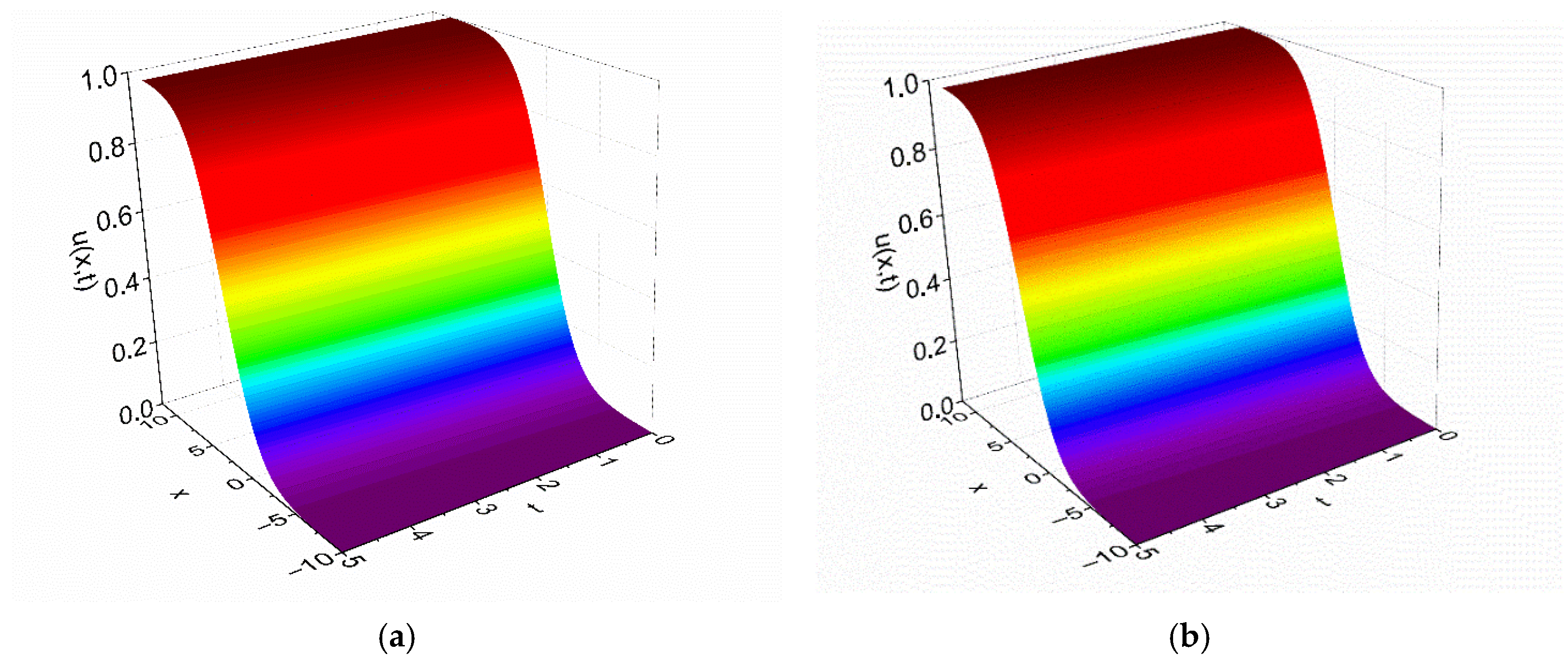
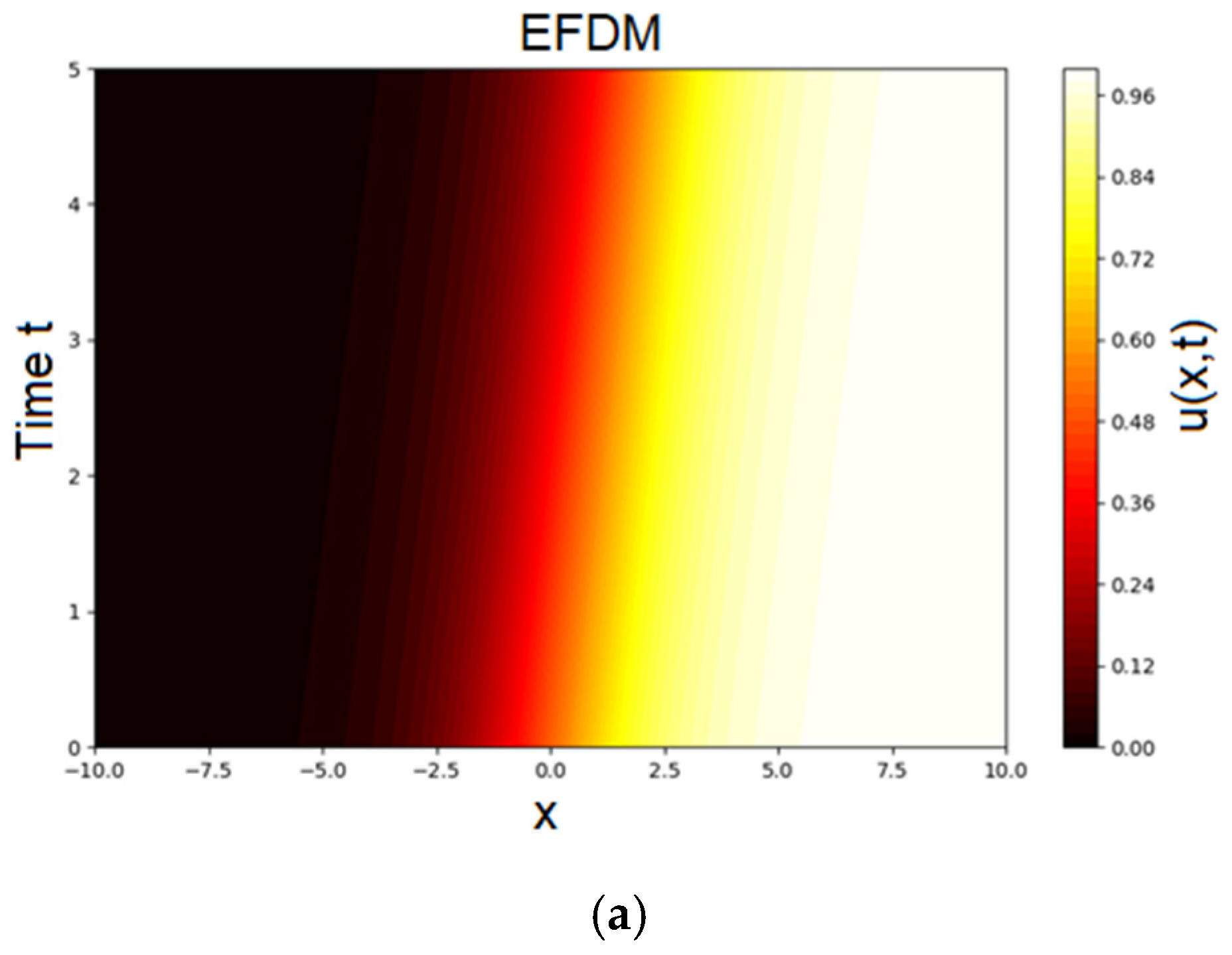
Although a good agreement between our numerical solutions and analytical solution can be seen, it is important to emphasize that the PINN provides a better fit with the analytical solution. Figure 2 provides a further demonstration of the physical behavior of the EFD and PINN solutions to Test Problem 1 in 3-dim. Figure 3 shows a heatmap of the predicted solution u(x, t) over the full space–time domain for Test Problem 1.

Test Problem 2: Consider the FHN Equation (1a) with $\alpha \left(t\right)=-\cos \left(t\right), \beta \left(t\right)=-\cos \left(t\right), \gamma \left(t\right)=-2\cos \left(t\right),$ the initial condition

$$u\left(x,t=0\right)={\displaystyle \frac{\mu }{2}}+{\displaystyle \frac{\mu }{2}}\mathrm{t}\mathrm{a}\mathrm{n}\mathrm{h}\left({\displaystyle \frac{\mu x}{2}}\right),-10\le x\le 10$$

(16)

and boundary conditions

$$u\left(x=-10,t\right)={\displaystyle \frac{\mu }{2}}+{\displaystyle \frac{\mu }{2}}\mathrm{t}\mathrm{a}\mathrm{n}\mathrm{h}\left({\displaystyle \frac{\mu }{2}}(-10-\left(3-\mu \right)\sin \left(t\right))\right), 0<t\le T$$

(17a)

$$u\left(x=10,t\right)={\displaystyle \frac{\mu }{2}}+{\displaystyle \frac{\mu }{2}}\mathrm{t}\mathrm{a}\mathrm{n}\mathrm{h}\left({\displaystyle \frac{\mu }{2}}(10-\left(3-\mu \right)\sin \left(t\right))\right), 0<t\le T$$

(17b)

The analytical solution of the problem is given as [8]

$$u\left(x,t\right)={\displaystyle \frac{\mu }{2}}+{\displaystyle \frac{\mu }{2}}\mathrm{t}\mathrm{a}\mathrm{n}\mathrm{h}\left({\displaystyle \frac{\mu }{2}}(x-\left(3-\mu \right)\sin \left(t\right))\right)$$

(18)

Test Problem 2 models a traveling wave in an excitable medium that oscillates periodically over time, capturing how signals or disturbances can speed up, slow down, or reverse under rhythmic forcing. This behavior appears across many real-world systems: in neuroscience, it reflects neurons responding to periodic inputs, influencing spike timing and synchronization; in cardiac tissue, it represents pacemaker-driven excitation waves and helps study arrhythmias; in chemistry, it describes oscillating reaction fronts under external forcing, such as in Belousov–Zhabotinsky reactions; in ecology, it models population waves affected by seasonal or cyclical environmental changes; and in engineering and materials science, it illustrates nonlinear wave propagation in semiconductors, plasmas, or memristive devices under periodic driving. Overall, the problem provides a controlled setting to test numerical and machine learning methods on non-stationary, periodically forced waves, linking mathematical theory to practical excitable systems.

The EFD solution of this test problem is given as

$${\displaystyle \frac{u_i^{j+1}-u_i^j}{∆t}}=-\cos \left(t_j\right){\displaystyle \frac{u_{i+1}^j-{{2u}_i^j+u}_{i-1}^j}{{\left(∆x\right)}^2}}-\cos \left(t_j\right){\displaystyle \frac{u_{i+1}^j-u_{i-1}^j}{2∆x}}-2\cos \left(t_j\right)\left({\left(u_i^j\right)}^3-{\left(u_i^j\right)}^2\left(1+\mu \right)+{\mu u}_i^j\right)$$

(19a)

$$\begin{gathered} { u}_i^{j+1}=u_{i-1}^j\left({\displaystyle \frac{\cos \left(t_j\right)∆t}{2∆x}}+{\displaystyle \frac{\cos \left(t_j\right)∆t}{{\left(∆x\right)}^2}}\right)+u_i^j\left(1-{\displaystyle \frac{2\cos \left(t_j\right)∆t}{{\left(∆x\right)}^2}}-2\mu \cos \left(t_j\right)∆t\right)- \\ 2{\cos \left(t_j\right)∆t\left(u_i^j\right)}^3+2{\left(u_i^j\right)}^2\left(1+\mu \right)\cos \left(t_j\right)∆t+u_{i+1}^j\left({\displaystyle \frac{-\cos \left(t_j\right)∆t}{2∆x}}+{\displaystyle \frac{\cos \left(t_j\right)∆t}{{\left(∆x\right)}^2}}\right) \end{gathered}$$

(19b)

The initial condition (16) in terms of finite differences becomes

$$u_i^1={\displaystyle \frac{\mu }{2}}+{\displaystyle \frac{\mu }{2}}\mathrm{t}\mathrm{a}\mathrm{n}\mathrm{h}\left({\displaystyle \frac{\mu x_i}{2}}\right), -10\le x_i\le 10, i=1, 2,\dots ,K (t=0)$$

(19)

and boundary conditions (17) are given as

$$u_1^j={\displaystyle \frac{\mu }{2}}+{\displaystyle \frac{\mu }{2}}\mathrm{t}\mathrm{a}\mathrm{n}\mathrm{h}\left({\displaystyle \frac{\mu }{2}}\left(-10-\left(3-\mu \right)\sin \left(t_j\right)\right)\right), j=1, 2,\dots ,M (x=-10)$$

(20a)

$${ u}_K^j={\displaystyle \frac{\mu }{2}}+{\displaystyle \frac{\mu }{2}}\mathrm{t}\mathrm{a}\mathrm{n}\mathrm{h}\left({\displaystyle \frac{\mu }{2}}\left(10-\left(3-\mu \right)\sin \left(t_j\right)\right)\right), j=1, 2,\dots ,M (x=10)$$

(20b)

One should mention that we used one-sided second-order differences for the advection term at two boundaries, in the following form:

$${\left.{\displaystyle \frac{\partial u\left(x,t\right)}{\partial x}}\right|}_{i=1}=(-3u_1+4u_2-u_3)/(2∆x)$$

(21a)

and

$${\left.{\displaystyle \frac{\partial u\left(x,t\right)}{\partial x}}\right|}_{i=K}=(3u_K-4u_{K-1}+u_{K-2})/(2∆x)$$

(21b)

where $u_1$ and $u_K$ are given in Equation (20a) and Equation (20b), respectively. Compared to the alternative choice of ghost nodes, one-sided second-order differences provide a much better propagation, preserving amplitude and speed. The truncation error for the difference Equation (21a,b) is O((Δx)²).

A comparison of the numerical solutions to Test Problem 2 obtained by the EFDM (step lengths are Δx = 0.5 and Δt = 0.0001) and PINN with the analytical solution (18) at different times T, by taking the parameter $\mu =0.75,$ is shown in

Table 5. Comparison of numerical and analytical solutions of Test Problem 2 for T = 0.001.

x	EFDM Solution	PINN Solution	Analytical Solution
−10	0.000414	0.000417	0.000414
−8	0.001851	0.001843	0.001851
−6	0.008226	0.008229	0.008226
−4	0.035512	0.035523	0.035512
−2	0.136630	0.136634	0.136630
0	0.374685	0.374605	0.374684
2	0.612992	0.613080	0.612992
4	0.714373	0.714295	0.714373
6	0.741745	0.741806	0.741746
8	0.748142	0.748114	0.748142
10	0.749585	0.749590	0.749585

(for T = 0.001),

Table 6. Comparison of numerical and analytical solutions of Test Problem 2 for T = 0.01.

x	EFDM Solution	PINN Solution	Analytical Solution
−10	0.000408	0.000409	0.000408
−8	0.001823	0.001815	0.001824
−6	0.008103	0.008105	0.008104
−4	0.034999	0.035013	0.035002
−2	0.134936	0.134945	0.134942
0	0.371852	0.371760	0.371836
2	0.611284	0.611369	0.611283
4	0.713848	0.713777	0.713854
6	0.741618	0.741681	0.741621
8	0.748110	0.748088	0.748114
10	0.749578	0.749584	0.749578

(for T = 0.01), and

Table 7. Comparison of numerical and analytical solutions of Test Problem 2 for T = 0.05.

x	EFDM Solution	PINN Solution	Analytical Solution
−10	0.000381	0.000378	0.000381
−8	0.001704	0.001701	0.001705
−6	0.007576	0.007581	0.007580
−4	0.032802	0.032828	0.032818
−2	0.127608	0.127636	0.127636
0	0.359272	0.359136	0.359196
2	0.603507	0.603571	0.603493
4	0.711434	0.711387	0.711461
6	0.741033	0.741097	0.741043
8	0.747975	0.747959	0.747983
10	0.749549	0.749551	0.749549

(for T = 0.05). Further reducing Δt and Δx did not lead to an improvement in the accuracy of the numerical solution.

Table 8. The accuracy of EFDM and PINN of Test Problem 2 at different times T.

T	Error (EFDM)	Error (PINN)
0.001	4.2640 × 10−7	4.7383 × 10−5
0.01	5.7604 × 10−6	4.6345 × 10−5
0.05	2.6836 × 10−5	4.1321 × 10−5

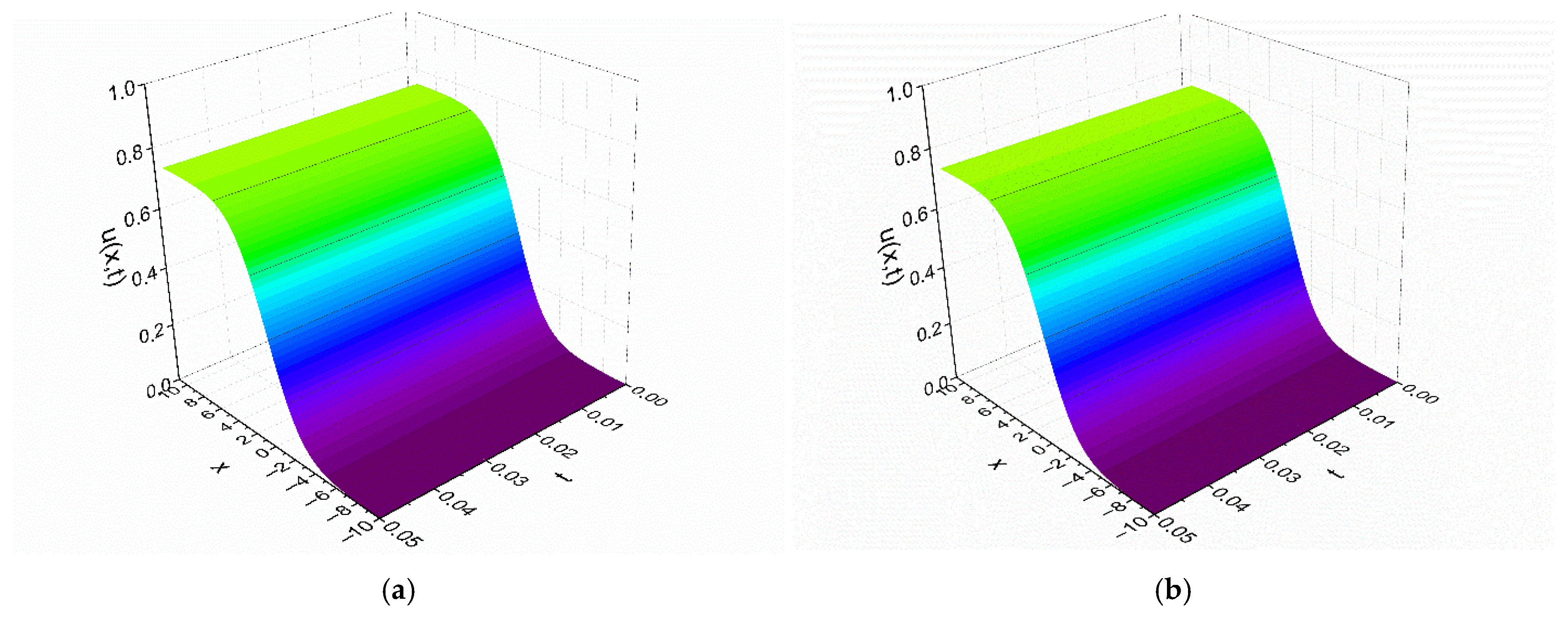
displays the accuracy of the EFDM and PINN in solving Test Problem 2 at various points in time. Although a good agreement between our numerical solutions and analytical solution can be seen, it is important to emphasize that the EFDM provides a better fit with the analytical solution. Figure 4 provides a further demonstration of the physical behavior of the EFD and PINN solutions to Test Problem 2 in 3-dim. 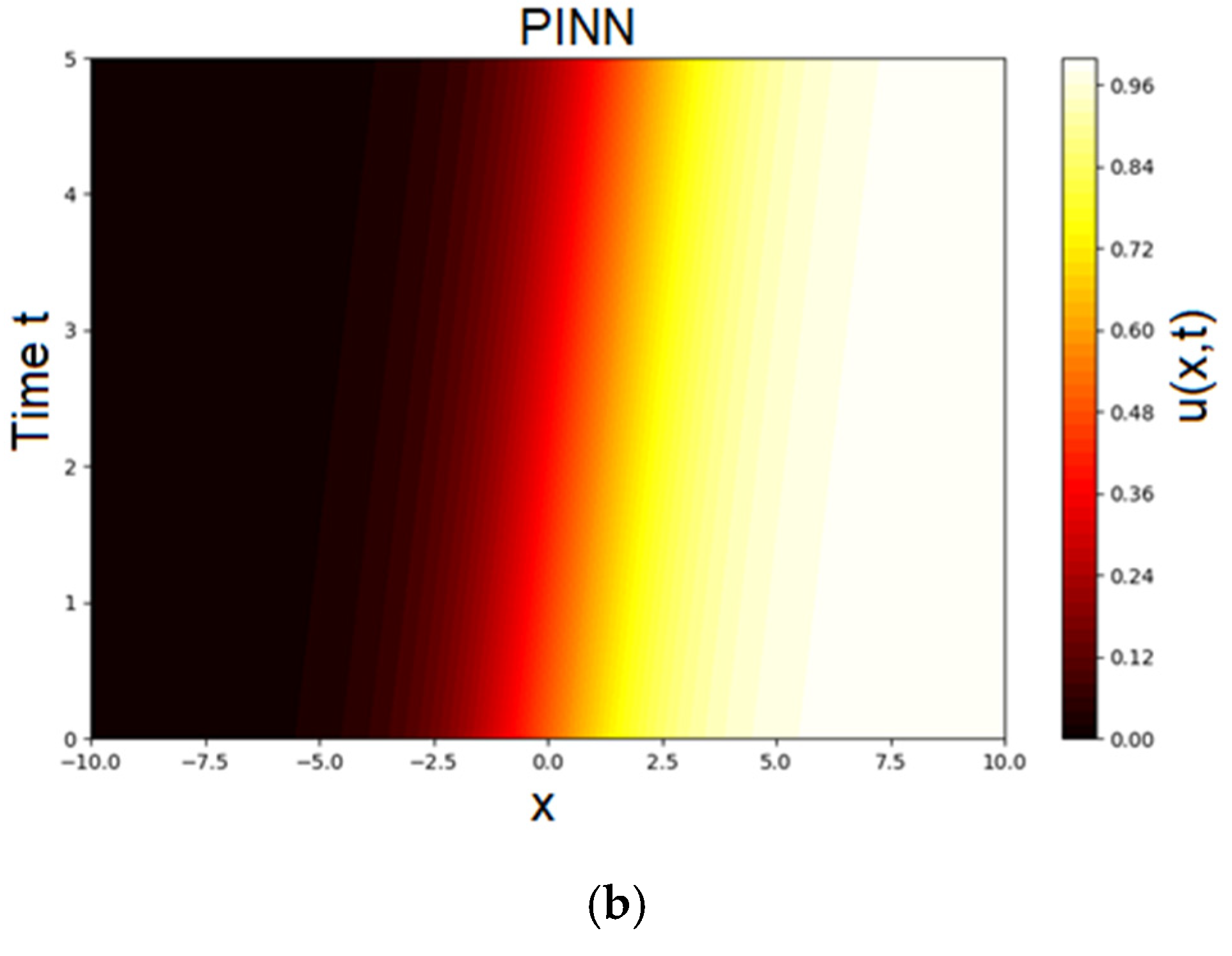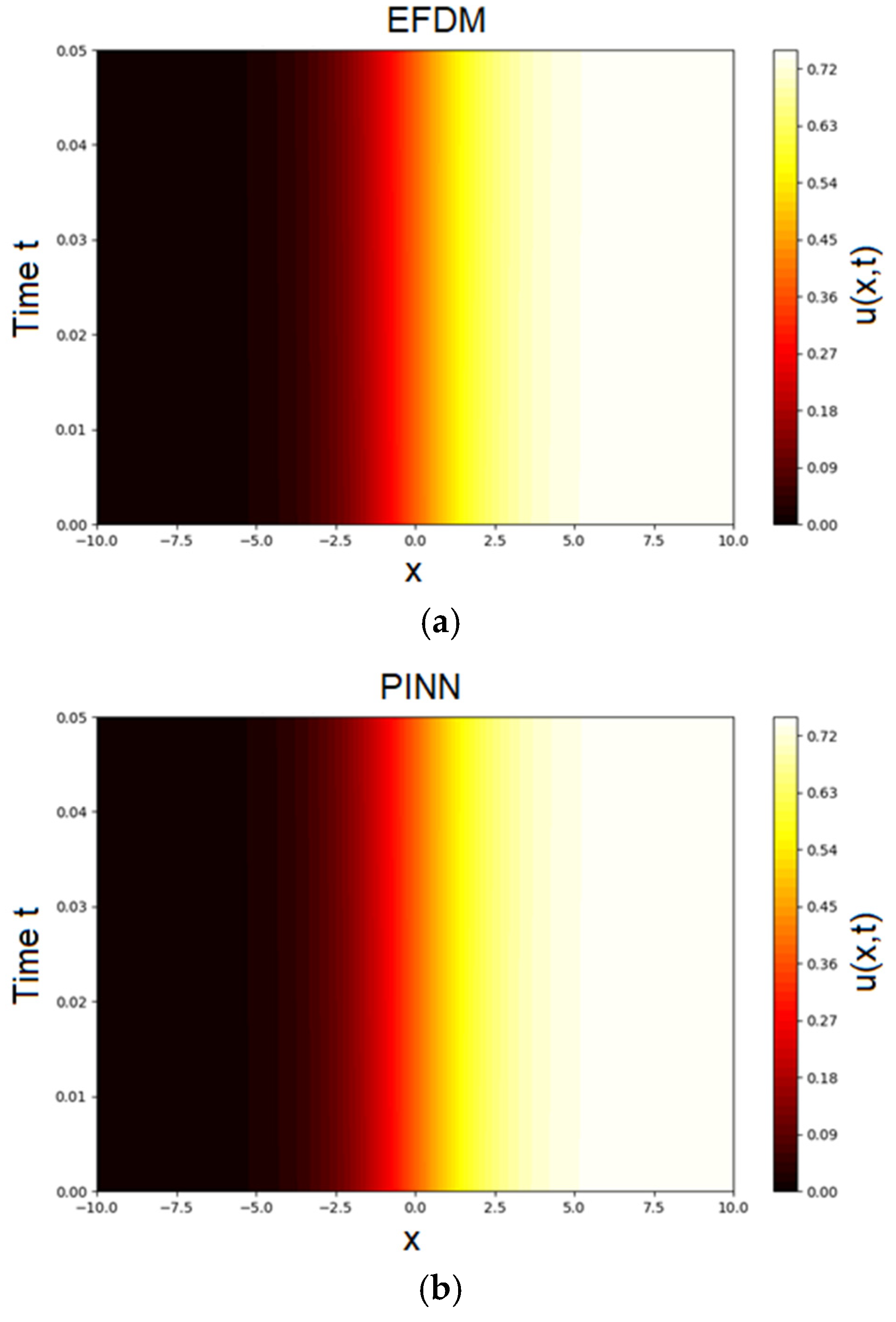Figure 5 shows a heatmap of the predicted solution u(x, t) over the full space–time domain for Test Problem 2.

6. Accuracy Assessment of EFDM and PINN

We conducted a brief grid/time refinement study for EFDM, using L² error as a measure of accuracy:

$$L^2 \mathrm{e}\mathrm{r}\mathrm{r}\mathrm{o}\mathrm{r}=\sqrt{{\displaystyle \frac{1}{N}}{\sum }_{i=1}^N\left(u_{numerical}\right(x_i)-u_{analytical}(x_i){)}^2}$$

(22)

In both test problems, the rates are approximately 2, as expected from the order of the problem being solved (see

Table 9. Convergence analysis for Test Problem 1.

Grid	Δx	L2 Error	Rate
Δx, Δt	1.000	5.04 × 10−3	-
Δx/2, Δt/2	0.500	1.03 × 10−3	2.28
Δx/4, Δt/4	0.250	3.10 × 10−4	1.74

and

Table 10. Convergence analysis for Test Problem 2.

Grid	Δx	L2 Error	Rate
Δx, Δt	1.000	2.17 × 10−4	-
Δx/2, Δt/2	0.500	6.18 × 10−5	1.81
Δx/4, Δt/4	0.250	1.61 × 10−5	1.94

).

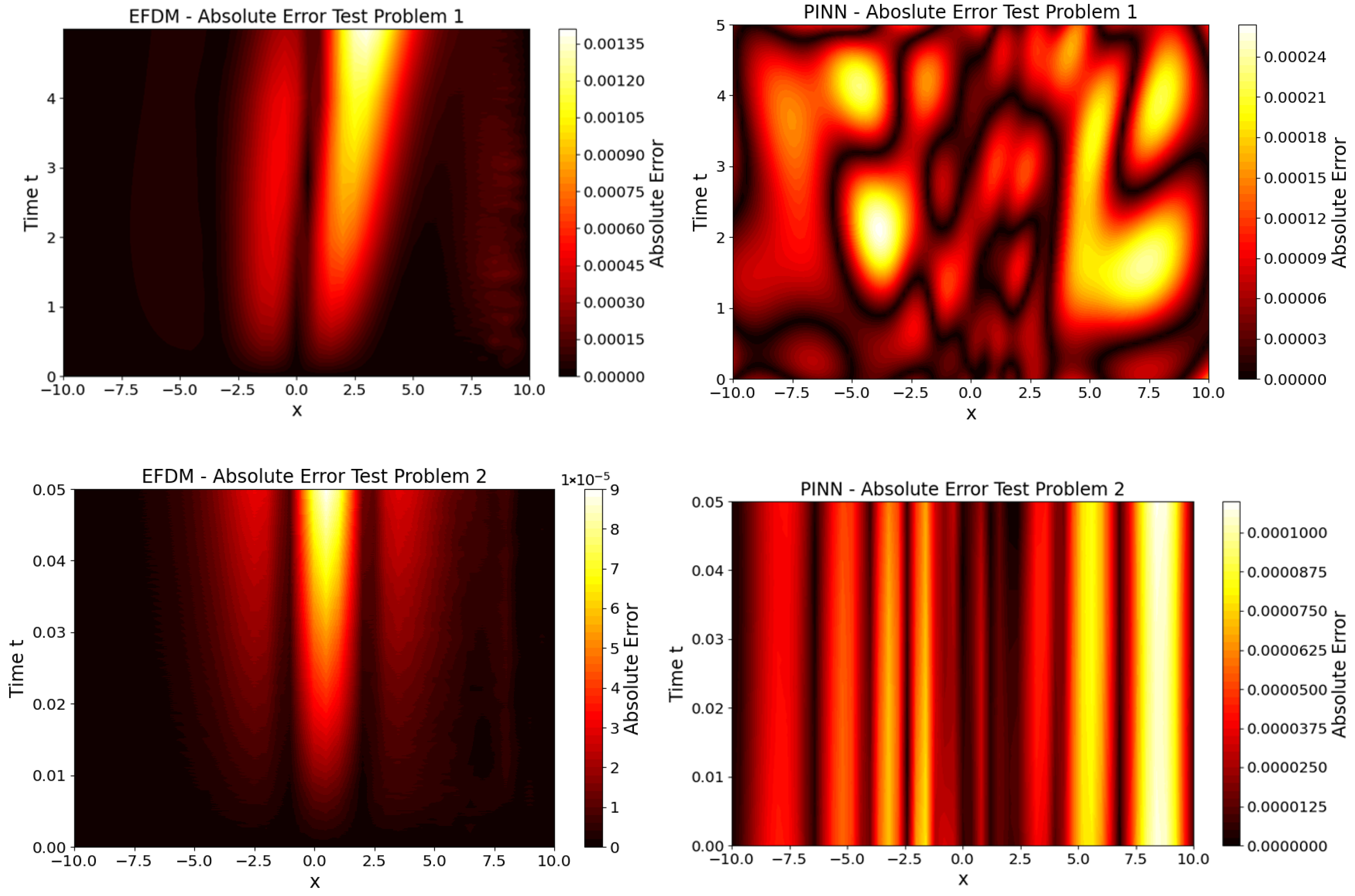
Figure 6 illustrates the integrated space–time L² error plot for EFDM and PINN. One can see from Figure 6 that quite different patterns for space–time L² error characterize EFDM and PINN. It can be seen that, for EFDM, areas with higher absolute error are concentrated towards higher values of t, while for PINN, the errors are evenly distributed. This happens because, in EFDM, the error accumulates due to the explicit time-stepping method, while in PINN, there is no classical time-stepping.

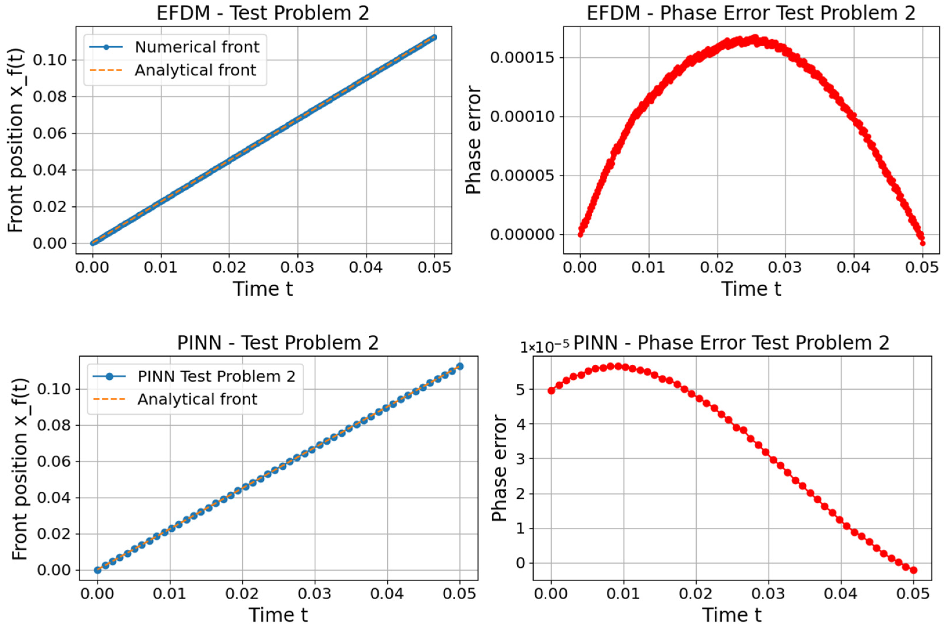
The phase error measures the timing/distance discrepancy in wave propagation. Figure 7 and Figure 8 show phase errors for traveling waves with front position $x_{f\left(t\right)}$, for Test Problems 1 and 2, respectively, calculated using the following equation:

$$\mathrm{p}\mathrm{h}\mathrm{a}\mathrm{s}\mathrm{e}\mathrm{e}\mathrm{r}\mathrm{r}\mathrm{o}\mathrm{r}\left(t\right)=x_{f_{numerical}\left(t\right)}-x_{f_{analytical}\left(t\right)}$$

(23)

The EFDM requires 1.1 s to solve Test Problem 1 (T = 0.05) and 21 s to solve Test Problem 2 (T = 5). These computation times are significantly shorter than the 85 s required by the PINN approach. Unlike EFDM, the PINN framework does not employ a classical time-stepping scheme; therefore, its total computational time corresponds solely to the training time of the PINN.

In Test Problem 2, although we admit time-varying coefficients α(t), β(t), and γ(t), the tests still follow smooth traveling-wave tanh profiles. In general, using smooth traveling-wave profiles (e.g., tanh functions) with time-varying coefficients α(t), β(t), and γ(t) simplifies the FHN model, focusing on core dynamics like wave propagation and the effects of time-varying parameters, while avoiding the complexities of pulse formation and front interactions. Stiffer, multi-scale, or pattern-forming dynamics require more advanced numerical methods and greater computational resources, so avoiding them helps reduce complexity and computational cost. In many real-world applications, such as real-time simulations or large-scale modeling, smoother, simpler profiles are more practical. While pattern formation and front interactions are relevant in some biological contexts, many systems do not exhibit these behaviors unless under specific conditions. By starting with smoother dynamics, one aligns with more controlled experimental setups or theoretical models where the system behaves in a simpler, steady-state regime. Early testing with simpler cases ensures the accuracy of numerical methods, allowing one to scale up to more complex systems later. In cases like neural or cardiac modeling, where wave propagation is often smooth, focusing on smoother dynamics better represents these scenarios.

Finally, to the best of our knowledge, we compare the accuracy of the EFDM and improved PINN approach for solving the FHN equation in this work. We obtained that, for solving the FHN equation, the PINN approach demonstrates better accuracy than numerical solutions produced by EFDM. It should be noted that the PINN approach is one or even two orders of magnitude more computationally demanding than the EFDM. In our previous work, we demonstrated that the EFDM outperforms the PINN approach in terms of accuracy when solving Burgers’ equation [15] and the Sine-Gordon equation [16]. PINN outperforms EFDM for the FHN equation because its smooth, dissipative, and stiff nature aligns with the strengths of NN-based smooth approximations and global optimization. 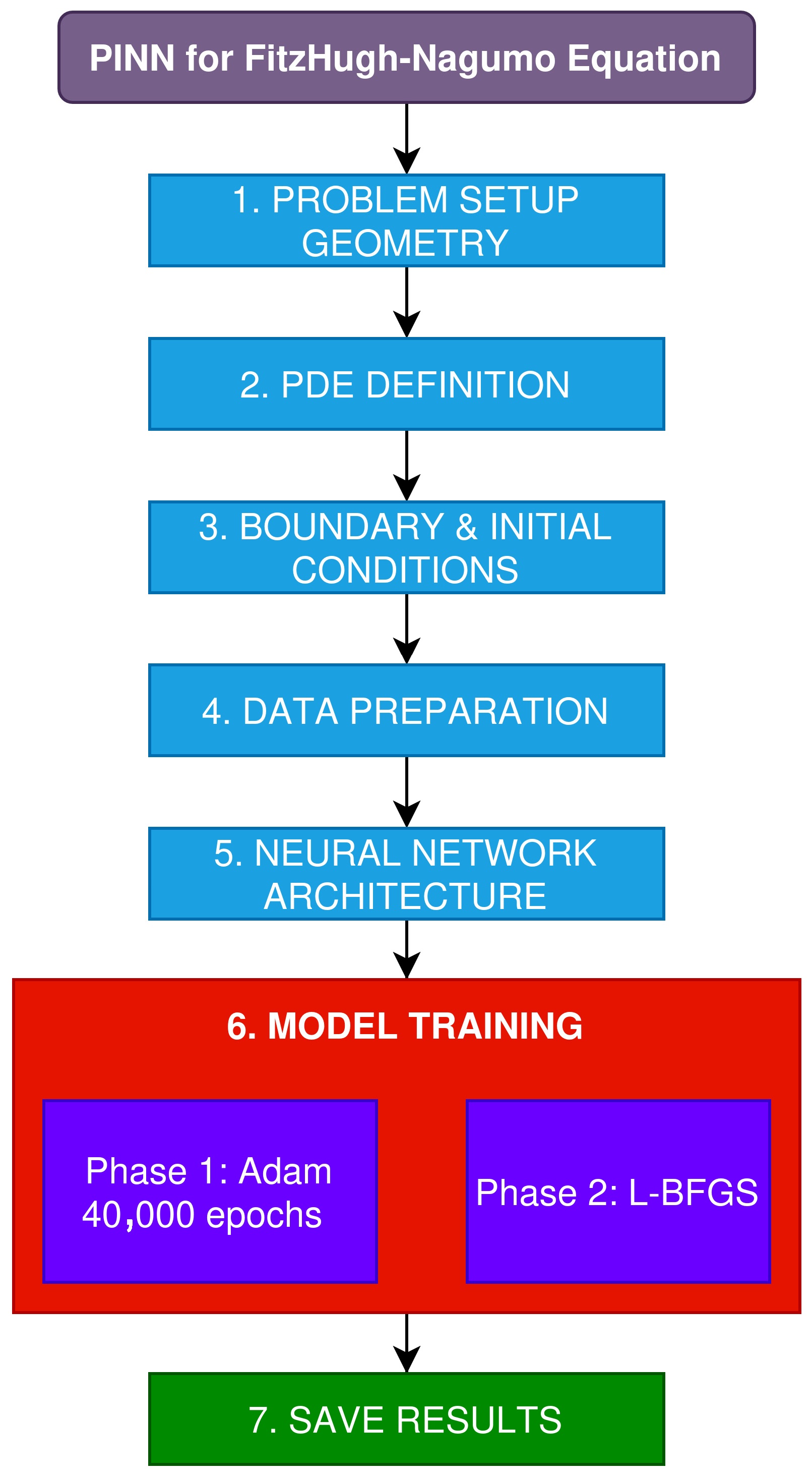In contrast, Burgers’ and Sine–Gordon equations involve shocks or oscillatory conservative dynamics, where traditional numerical schemes better preserve sharp or oscillatory structures, while PINNs’ smooth approximators struggle [15,16]. The results of this study are particularly important for assessing the performance of the PINN in solving the FHN equation, especially for various nonlinear physical processes. These processes include phenomena such as pulse propagation in optical fibers, geophysical fluid dynamics, and long-wave propagation in both shallow and deep ocean environments. This highlights the potential of PINNs to handle complex, nonlinear systems, despite their initial limitations compared to EFDM. The PINN flowchart used in this work is shown in Figure 9.

Finally, while the classical FHN model captures the basic excitability of neurons and other excitable media, real-world systems are often far more complex. In such systems, singularities naturally arise due to the interplay of multiple timescales, strong nonlinearities, and spatial or network interactions. Fast–slow dynamics, for instance, create regions where the state variables change abruptly over very short spatial or temporal scales, producing boundary layers or spike bursts that cannot be captured by the simple smooth FHN equations. Discontinuous or piecewise nonlinearities further introduce singular points in the system, where the derivative of the response changes suddenly, modeling threshold-like behavior observed in real neurons, cardiac tissue, and chemical reactions. High-dimensional extensions of FHN, such as coupled networks or spatially extended reaction–diffusion systems, produce singular wave phenomena including spiral cores, wave collisions, and reentrant patterns, all of which play a central role in arrhythmias, seizure dynamics, and pattern formation in chemical media. In addition, stochastic perturbations or external forcing can amplify these singular behaviors, leading to complex phenomena like chaotic bursting or wavefront breakup. From a numerical standpoint, singularities present significant challenges. Standard explicit methods may become unstable or fail to resolve sharp gradients, while naive discretization can smear essential features of the solution. Accurate simulation requires adaptive time-stepping, mesh refinement, or specialized singular perturbation techniques, and these approaches must balance computational efficiency with the need to capture critical dynamical features. Ultimately, studying singular FHN-type models provides deeper insight into the rich dynamics of excitable systems, revealing mechanisms behind rhythmic bursting, conduction block, pattern formation, and nonlinear wave interactions that the classical smooth FHN model cannot represent. By incorporating singularities, these models bridge the gap between idealized theory and the complex behaviors observed in biology, chemistry, and materials science.

7. Conclusions

We compared the analytical solutions that had previously been reported in the literature with our numerical results for the solution of the nonlinear parabolic differential equation of the FHN type, which we obtained using the improved PINN and standard EFD approach. While both approaches provide good agreement with analytical solutions, our findings reveal that the PINN method aligns more closely with the analytical solutions in Test Problem 1, whereas the EFDM achieves higher accuracy in Test Problem 2. This study is key to assessing the PINN’s effectiveness in solving the FHN equation and its application to nonlinear phenomena, such as pulse dissipative dynamics in optical fibers, drug delivery, neural behavior, geophysical fluid dynamics, and long-wave propagation in oceans, showcasing the potential of PINNs for tackling complex systems. The principles underlying the methods of solution employed in this study may be used to create numerical models for nonlinear PDEs employed for the investigation of a wide range of nonlinear physical processes in physical and engineering problems.