Abstract
It is demonstrated that the general representation of a dynamic multiphase wellbore flow model may be identified from the available physical measurements. The proposed approach is based on the techniques of numerical optimization and also requires the availability of solvers for the general type of partial differential equations describing two-phase gas–oil flow. A solution is obtained both for the case of the homogeneous no-slip model and the drift-flux model with velocity slip. The feasibility of the proposed approach for system identification and parameter estimation has been demonstrated using simulated flow data. Two distinct scenarios have been considered: firstly, when the well is fully instrumented with multiple pressure sensors and a multiphase flow meter, and secondly, when only a single downhole pressure gauge is available.
1. Introduction
The growing gap between the demand and supply of hydrocarbons remains one of the most important challenges in the modern oil and gas industry. While the depletion of traditional reserves is observed, the development of unconventional resources is still questionable from an economic perspective. In order to address these challenges, advanced reservoir management strategies [1] are often used. These strategies in turn rely on the availability of advanced modeling tools, which adequately describe the hydrocarbon recovery process [2,3]. In particular, modeling of multiphase wellbore flow ensures that the hydrocarbons are transmitted economically from the reservoir to the end user during all the stages of a project including drilling [4], production [5] and transportation to the processing facilities [6]. Knowledge of produced oil, gas, and water rates is critical for production optimization, rate allocation, and flow assurance. It also helps to identify and mitigate production instabilities, such as gas or water breakthrough [7], or prevent certain undesired flow regimes, e.g., severe slugging [8]. It is also possible to determine the individual contribution of inflow intervals and wells to the total production using a model-based approach. Finally, the models of multiphase transport help to estimate risks from hydrate and paraffin deposition and facilitate the choice of an optimal chemical inhibitor. To summarize, dynamic multiphase flow modeling can support the whole range of wellbore-related operations in the oil and gas industry.
There are several approaches to how these predictive models can be formulated. Firstly, such models are formulated with known physical laws or empirical relationships, which results in representing a specific physical process by a set of algebraic or differential equations or a combination of both. This solution is widely used due to the transparent reasoning behind it, though as such it does not guarantee that the obtained equations are fully applicable to a specific scenario, as they can be based on wrong assumptions. In order to mitigate these limitations (and also due to the rapid development of computational methods), another approach has recently emerged, where the predictive model is obtained directly from the data so that the formulation is based on the observed behavior rather than a priori knowledge and assumptions [9,10]. The main advantage of data-driven methods is the high accuracy of obtained models for the wide range of applicable conditions. The main disadvantage of the data-driven approach is the lack of generality and problems with extrapolation of the data outside the training range. That is, the flow model developed for a section of a horizontal well will be drastically different from a vertical one. It is impossible to adapt such a model without an inclination angle as an additional input parameter, and the development of a new model might be required. Therefore, fully ignoring the underlying physics may lead to significant uncertainty, especially if the model needs to be rescaled.
The disadvantages of both approaches discussed above can be mitigated by introducing a hybrid solution, where the general form of the governing equations is defined by physical laws but the detailed description is derived from the data [11,12]. Combining data and physics is particularly important for the equations with significant uncertainty, such as the experimentally derived empirical relationships (e.g., friction factor as a function of flow velocity [13]). In addition, some mathematical models that account for multiple phenomena on different scales are too detailed for practical applications. In this case, the simplest formulation is often required, which is achieved by omitting the negligible terms in accordance with the available measurements. As an example, fluid flow in porous media can be well described by Darcy’s law, though in some specific cases additional terms can be required [14]. On the other hand, the uncertainty associated with generally known conservation laws (such as continuity equations) or the gas equation of state is insignificant, and mathematical formulation is justified without any corrections by data.
In this work, such a hybrid solution is introduced, where the general form of governing equations is obtained directly from data. This step follows the ideas in [15], where the process model has been derived in the form of conservation equations. The values of closure parameters of the model are then additionally estimated using an optimization routine. While the methods presented in this paper are generic, the considered use case deals with the specific problem of identification of a dynamic multiphase wellbore flow model. The practical importance of such a problem is that the availability of accurate models is essential for agile and accurate hydrocarbon production management both on the scale of a single wellbore and a whole oilfield [16]. It is also important to note that as most of the measurement equipment is installed in the wellbore, there is an explicit relationship between the data from the sensors and flow-related variables making it especially attractive for such model validation. In addition, the number of sensors is limited, and it has a direct impact on the amount of data available. This limits the option of using a well-defined technique for model identification based on sparse regression [17,18], where it is assumed that the solution of the equations can be represented as known functions of both time and coordinate. In contrast, in the current work, an extreme scenario is considered when only a single pressure gauge is installed, resulting in the absence of spatial measurements. The possibility of dynamic model identification under conditions of limited data availability and model uncertainty defines the scientific challenge addressed in the current work. It should be mentioned that neither equation reconstruction nor parameter estimation is novel, and there are multiple applications of these methods in oil and gas and other industries. But ultimately, it is a combination of these techniques that facilitates the development of new modelling tools for multiphase wellbore flow directly from data.
The paper is organized as follows: first, the physical flow model of two-phase wellbore flow is introduced. This is followed by the formulation of a reconstruction problem, where the physical flow model is defined from data. This is followed by a series of computational examples, which illustrate the feasibility of the proposed approach. The problem of measurement availability is also addressed in the current work, where scenarios with different sets of installed sensors are considered. The paper ends with the conclusions and recommendations for future work.
2. Dynamic Model of Two-Phase Wellbore Flow
The analysis is based on a traditional hydrodynamic approach [19] to describe the flow of two-phase fluid in a wellbore with length L, which is deviated from a vertical by an angle θ (Figure 1). By averaging all the flow variables over a cross-section of a well, the problem can be effectively considered as one-dimensional. The flow is then characterized by the following variables, which are coordinate- and time-dependent: velocities of gas vg and oil vl, volumetric phase fractions of gas αg and oil αl, and single pressure p. The phase fractions are related to each other through the following geometrical relationship:
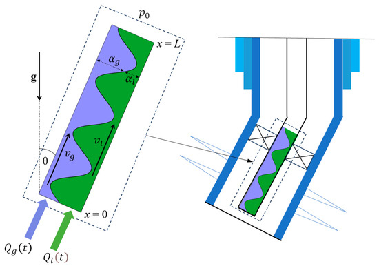
Figure 1.
Schematic description of a deviated producing well characterized by a one-dimensional multiphase flow model.
The oil phase is considered as an incompressible fluid characterized by a constant density ρl, and the ideal equation of state is applied for gas
where μ—molar gas mass, T—temperature, Rg—universal gas constant. Mass conservation is represented by a continuity equation formulated for each phase:
In addition to Equations (1)–(4), it is required to add two additional relationships describing momentum conservation for oil and gas. This would require explicit formulation of wall friction for each phase and mutual interaction between oil and gas. Instead, a drift-flux approach is being used [20,21] where the fluids are treated as the mixture. That results in a single momentum equation formulated as:
where
Here, v and ρ refer to mixture velocity and mixture density, respectively. The last term on the right-hand side of Equation (5) corresponds to the pressure frictional losses. Parameter k depends on the wellbore diameter, length, and Reynolds number [11]. However, to support the feasibility analysis of a newly introduced method, it is assumed that this parameter is constant. System of Equations (1)–(7) requires a closure relationship, which in the case of a drift-flux model is given by an algebraic slip law defining gas velocity vg as a function of mixture velocity v [20]:
In a general case, the parameters C and vd are flow related and can be defined by various empirical correlations [21]. Since both the distribution parameter and drift velocity can vary with significant changes in αg, v, the resulting slip law is represented by a complex non-linear function. However, for baseline calculations, these parameters have been selected to be constant in this study, and investigation into more complex scenarios is left for future work. This is just a rough approximation of reality, as generally speaking they are flow-regime dependent and may vary within the same flow pattern.
In addition, the system of governing Equations (1)–(8) requires boundary and initial conditions for closure. The inlet boundary conditions (at x = 0) are represented by the inflow mass flow rate for each phase per unit area:
The outlet boundary condition (at x = L) is defined by a constant wellhead pressure:
The initial condition at t = 0 is calculated from a steady-state solution of Equations (1)–(8) for some constant values of inflow rates Qg(0) and Ql(0).
3. Formulation of the Equation Reconstruction Problem
The main source of uncertainty of the system Equations (1)–(8) is associated with momentum Equation (5) and slip law Equation (8). Actually, Equations (1), (6), and (7) are obtained from the physical background of underlying variables. Mass conservation Equations (3) and (4) are valid in the presented form if no additional mass transfer is present. However, following the formulation from [19,20], this effect is omitted in the considered case. At the same time, Equations (5) and (8), which constitute the core of the drift-flux approach, are obtained under severe assumptions and only approximately describe the flow. Hence, it is the mixture momentum Equation (5) and slip law Equation (8) that need to be reconstructed based on the available measurements. As the proposed method does not depend on the number of equations involved, the current work concentrates on identification of the momentum equation only. This in particular would allow us to consider a special case of homogeneous no-slip flow where velocities of both phases are the same (C = 1, vd = 0 in Equation (8)). The terms and in Equation (5) refer to the flow dynamics and the effect of the pressure field on fluid flow. Obviously, they need to be included in the momentum Equation (5) as such (though there are models where the term is omitted due to its small quantity [19]). The remaining three terms need to be validated: represents the convection, but it can be neglected at low velocities due to its quadratic dependence, depends on the inclination angle, which is known to a limited extent, and is an approximate relationship for the frictional losses. The latest issue is especially important as the uncertainty in friction description may result in additional terms, which depend on (similarly to Brinkman extension of Darcy law [14,22]). Therefore, the general formulation of the momentum equation is given by the following equation:
Here F refers to some unknown function, which needs to be identified through an equation reconstruction process.
The measurements, which are required for model identification, should be related to the values of independent variables vg, vl, αg, αl, and p. The first four are obtained from a multiphase flow meter, which enables phase fraction measurements and the last one is obtained from the pressure gauge. For practical applications, it means that a complete set of measurements is represented by multiple pressure sensors installed along the length of the well and a multiphase flow meter at the wellhead. Then, at a given time instant t, the measurements include the values of v and αl at x = L and p at any given coordinate. The opposite scenario is when only a single downhole pressure gauge is installed, then the measurements are represented by pressure p at x = 0, which corresponds to the minimal viable measurement layout.
Therefore, the reconstruction problem can be reformulated in the following way: it is necessary to define function F in such a way that the solution of the system Equations (1)–(11) is consistent with the available measurement data in all time instants t, which are obtained in either of two scenarios defined above.
4. General Approach to Equation Reconstruction
It is ultimately required that the relationship (11) obtained through identification should have an explicit physical interpretation; therefore, it is feasible to define the unknown function F as a linear combination of n selected functions F1, F2, …, Fn, which constitute the library of possible terms:
Here c1, c2, …, cn are the coefficients of a linear combination that uniquely define function F. If these coefficients are known, then the system of equations defined above can be solved numerically, and then the simulation results can be compared with the readings from the installed pressure sensors. Then, the reconstruction problem can be formulated through the minimization of some residual R, which is a function of n variables c1, c2, …, cn. Numerical optimization of such a function would require calculation of values of the R function for a significant number of points in the subspace of parameters c1, c2, …, cn, with a direct solution of system Equations (1)–(11) needed for each of these points. Therefore, the effective application of the proposed approach to system reconstruction requires both a numerical solver and an optimizer to demonstrate efficient convergence. In the framework of the considered problem, the residual R is minimized by using a combination of the quasi-Newton method BFGS [23] and the Nelder–Mead algorithm [24], which are consequently applied: the first algorithm provides the estimate of the minimum, which is further used to initialize the second one, which ensures sufficient accuracy. At the same time, as the type of Equation (11) is not uniquely defined due to variation of the function F, the existing numerical methods for fluid dynamics (e.g., SIMPLE [20,25]) cannot be confidently used. To mitigate this, a few generic numerical solvers are suggested, which are discussed in Section 5.1 and Section 6.1.
The specific formulation of the residual R should be chosen in accordance with the number and type of sensors installed in the wellbore. In the case of a minimal viable scenario, where only downhole pressure readings are available, the following expression for the residual is used:
Here and below, the subscript «~» refers to the measurements, which are aggregated over all time instants when all these measurements are acquired. Residual (13) is basically a sum of relative mismatches between simulated and measured values. Then, the similar expression for the scenario with a fully instrumented well (a topside multiphase flow meter and multiple downhole pressure gauges) is defined as:
where points x = xj correspond to the positions of m sensors in a well. The coefficients c1, c2, …, cn are implicitly included in Equations (13) or (14), as their values unequivocally define the residual R, since the predicted values of p, v, and αl are obtained from the solution of the equation system represented by the linear combination of terms. Therefore, minimization of residual R as a function of multiple parameters c1, c2, …, cn, defines the problem of equation reconstruction. Formulating equation reconstruction as the optimization problem does not necessarily imply that a linear combination of terms is required. It is important to note that Equation (12) is formulated in such a way that any combination of terms is possible, and parameters c1, c2, …, cn could be on the right-hand side of Equation (12) in an arbitrary way. However, in the case of linear combination, obtaining zero values of some of the coefficients ci has a direct physical interpretation, as it means that a certain phenomenon defined by a function Fi has negligible impact on the flow process. The workflow for the equation reconstruction algorithm presented above can be summarized with the following steps:
- Select the library of potential terms Fi in Equation (12).
- Implement a numerical solver for Equation (11) that uses coefficients ci as input and returns the values of the variables p, v, and αl for all values of x and t.
- Implement the function R(c1, c2, …, cn) in a form of (13) or (14) that returns the value of residual based on the calculated values p, vk, and αl (Step 2) and known measurements.
- Set the initial values of the coefficients c1, c2, …, cn.
- Minimize numerically the implemented function R(c1, c2, …, cn) (see step 3) using the selected initial values of c1, c2, …, cn. Once the minimum of R is achieved, the corresponding values of the coefficients ci completely determine the form of function (12), and, therefore, the form of Equation (11).
5. Homogeneous Wellbore Flow
Firstly, a homogeneous flow is considered, which is characterized by C = 1, vd = 0. In this case it follows from Equations (1), (6), and (8) that vg = vl = v, meaning that both phases travel with the same velocity. This is a significant simplification, as it enables to dismiss Equations (6) and (8) from analysis. In addition, Equations (3) and (4) can be combined to formulate the mixture continuity equation:
Although the assumption of equal phase velocities is often unrealistic, the homogeneous flow model provides a baseline solution for the reconstruction process.
5.1. Numerical Solution of a Direct Problem for Homogeneous Model
A numerical method that is based on ideas of the iterative SIMPLE [25] approach is used to solve the direct problem defined in Section 2. A fully implicit time integration is applied, which facilitates the application of relatively large time-steps Δt = 0.05 s. The wellbore is discretized with 20 spatial grid blocks of equal size. Note that although the parameters of discretization are important features defining the stability of the numerical scheme used, the corresponding analysis is out of scope for this work. This is due to the fact that the presented results are more focused on the solution of the reconstruction problem rather than the evaluation of the stability and convergence properties of the numerical scheme. The considered equation system is linearized and transformed into a set of algebraic equations, which are solved using a control volume technique [26].
Solution of the direct problem firstly requires system initialization, which is performed from steady-state values as discussed above. By using Equations (3), (4), and (9) for an arbitrary value of x the following is obtained:
Equation (16) is valid for any formulation of slip law (8). For the case of homogeneous no-slip conditions, the initial distribution of mixture density is calculated by using (7) and (9):
With the help of Equations (16) and (17), Equation (11) is transformed into an ordinary differential equation for p(x), which is easy to solve. Mixture velocity distribution v(x) is calculated from (16) and volumetric volume fractions αl(x) and αg(x) from (9).
Afterwards, the calculation of p, v and αl for each time instant defined by a time step of Δt is performed. The iterative approach is used so that at each new time step t + Δt, the solution is initialized using known values obtained at previous time step t. The solution is obtained through the following process:
- (1)
- Equation (4) is solved for a new guess αl;
- (2)
- Equation (7) with (1) and (2) is used to calculate ρ;
- (3)
- Equation (15) is solved for a new guess v;
- (4)
- Equation (11) is solved for a new guess p.
The iterative process is converged when the variation of p, v and αl in each cell of the computational grid becomes negligible (the convergence criterion was set to 10−5 in the current study).
5.2. Equation Reconstruction Results for Homogeneous Model
The proposed method has been evaluated through a twin experiment approach, where the synthetically generated measurements are obtained by solving system Equations (1)–(8). This refers to the situation where Equation (5) is known, meaning that the reconstruction process should ultimately lead to the following formulation of the momentum equation:
The following values of parameters are used to generate true measurements: L = 1000 m, p0 = 105 Pa, μ = 0.029 kg/mol, T = 300 K, ρl = 850 kg/m3, g = 9.8 m/s2, θ = 0, k = 10 m−1. It is also assumed that the gas mass rate is constant Qg(t) ≡ 2 kg/(m2∙s). The oil flow rate is assumed to be initially constant and equal to 1000 kg/(m2∙s) afterwards, its value is gradually increased up to 1250 kg/(m2∙s) or 1500 kg/(m2∙s) during 0.1s, then it gradually decreased back to its initial value during the same time interval (Figure 2). This process resembles well control by manipulation of a wellhead choke. Disturbing the flow in such a way created transient flow behavior, which adds data relevant to flow dynamics in contrast to steady-state conditions. Two values of maximum flow rates are needed to provide a more elaborate dynamic response, as it will be demonstrated further that a single flow rate disturbance may not be sufficient to identify correctly all the coefficients in Equation (12). It is therefore suggested to first minimize a residual for the data corresponding to the first disturbance and then repeat the whole process for the second disturbance using the initially obtained coefficients ci as an input.
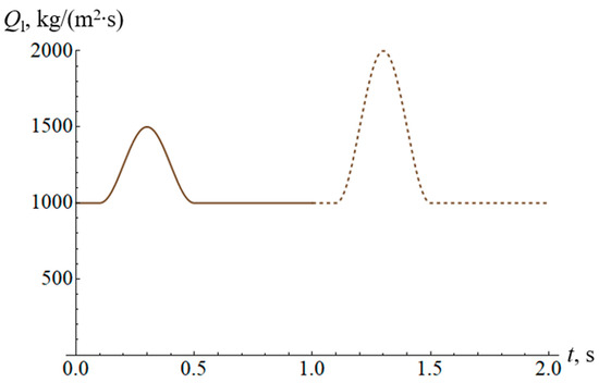
Figure 2.
Inflow oil rate (per unit area) as a function of time. The solid line refers to the first disturbance and the dashed one to the second.
Firstly, the library of n = 4 terms is used:
While terms F1, F2, and F3 correspond to gravity, convection, and friction, the last component of the library F4 is actually redundant. In fact, F4 corresponds to diffusion, which although it may be part of mathematical Equation (18), is in fact implicitly included in frictional losses. This is confirmed by the reconstruction process, where the scenario with maximum information available demonstrated convergence within 290 iterations. The resulting values of the coefficients of linear combination are c1 = 9.8, c2 = 1, c3 = 10, c4 = 0 for only the data associated with the first flow rate disturbance. The graphical representation of how the values of coefficients are calculated within the iterative process is given in Figure 3. In the scenario with minimum information a single disturbance is not sufficient as for 461 iterations, the obtained values of coefficients are far from the actual (in particular, c4 = 0.73). Repeating the optimization process with the second flow disturbance added decreases the uncertainty and allows us to obtain true values of coefficients for 252 iterations (Figure 4). The absolute error of the estimation, that is the difference between the predicted and true values of coefficients, is of order 10−7–10−8.
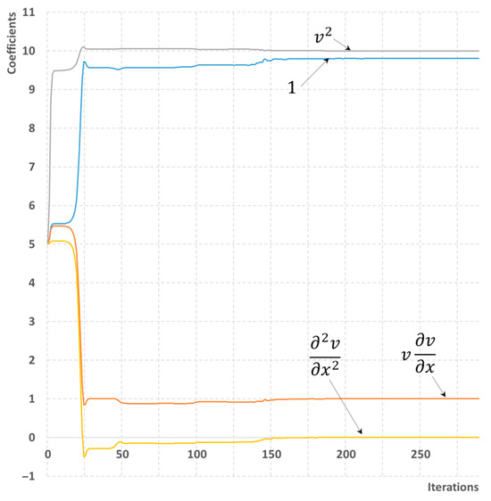
Figure 3.
A process of reconstructing the momentum equation for homogeneous flow. The library of four possible terms is used. The maximum number of sensors is available.
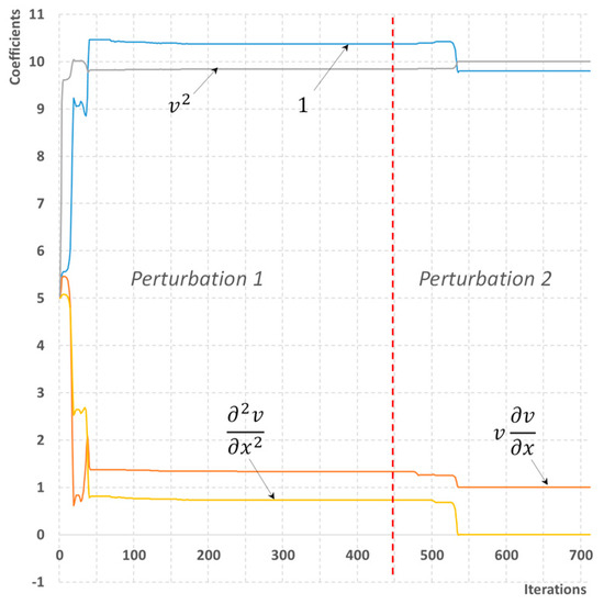
Figure 4.
A process of reconstructing the momentum equation for homogeneous flow. The library of four possible terms is used. The minimum number of sensors is available.
Next the expanded library of n = 6 terms is considered. Here, two additional terms are added, one directly proportional to mixture velocity and another to its derivative. Although both of these terms might be associated with certain physical phenomena, they are not observed in the framework of the one-dimensional drift-flux model.
In this case, even with two induced flow disturbances, the scenario with a single pressure gauge does not lead to accurate reconstruction. However, for the fully instrumented well, the correct values of coefficients are obtained within 823 iterations, which is significantly higher than using the reduced library defined by Equation (19). The evolution of the reconstructed coefficients as a function of iteration number is depicted in Figure 5 and Figure 6. It is demonstrated that within 400 iterations the qualitative representation of momentum Equation (11) can already be observed. The absolute error is of order 10−6–10−7.
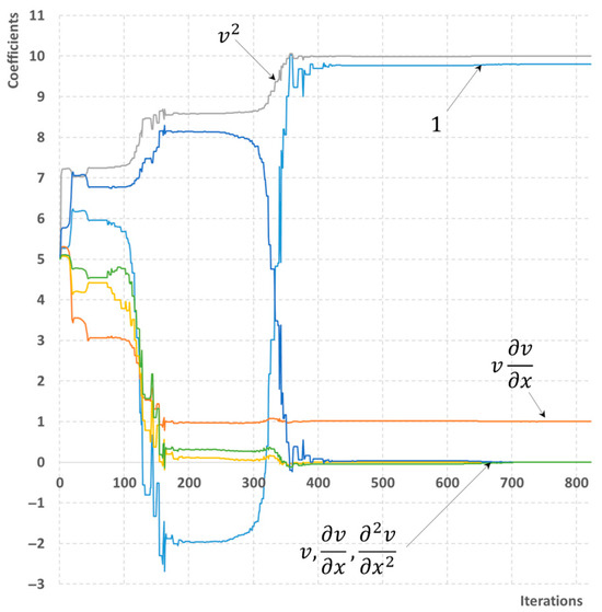
Figure 5.
A process of reconstructing the momentum equation for homogeneous flow. The library of six possible terms is used. The maximum number of sensors is available.
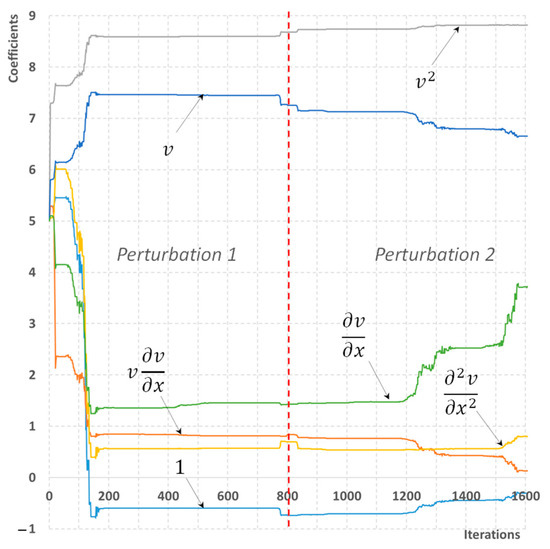
Figure 6.
A process of reconstructing the momentum equation for homogeneous flow. The library of six possible terms is used. The minimum number of sensors is available.
It can be concluded that expanding the library of potential terms would consequently require a more detailed measurement dataset; in particular, the information from additional sensors is needed, and the collected data needs to be significantly unsteady, which may be caused by natural flow phenomena or result from some external control. Although this is a natural conclusion, it could be noted that even for a library of four possible terms, the reconstruction with a single pressure sensor available fails without a second flow disturbance added. It is also anticipated that that expanding the number of terms would increase the computational cost of the optimization process, which is expressed in a longer convergence process. On the other hand, it is natural to take into consideration as many terms as possible as it enables a holistic representation of underlying flow equations.
6. Wellbore Flow with Slip
As discussed in Section 2, in a general case the parameters C and vd in Equation (8) can depend significantly on flow dynamic variables [16]. However, if their values are constant but different from the homogeneous case with C = 1, vd = 0, the phase velocities vg and vl are different due to slip between liquid and gas phases. At the same time, the relationship (15) becomes inapplicable and it needs to be replaced by the following formulation of mass conservation for the mixture:
where
represents the mass flow rate of the mixture of fluids.
6.1. Numerical Solution of a Direct Problem for Model with Slip
The initial conditions are obtained similarly to the homogeneous case, since Equation (16) remains valid even if the slip between phases is taken into account. However, the iterative process is slightly adjusted due to changes in the representation of the governing equation system. It is assumed that the state of the system is defined by p, v, and αl both at the beginning of the iterative process and its end as well.
- (1)
- vg is calculated from Equation (8);
- (2)
- vl is calculated from Equation (6) using obtained vg;
- (3)
- A new approximation for αl is obtained from Equation (4);
- (4)
- p is calculated from Equation (7) using (1) and (2);
- (5)
- Q is calculated from Equation (22);
- (6)
- Mixture velocity v is calculated from (6), (8) and (22) using calculated values of vg and vl;
- (7)
- A new approximation for p is obtained from Equation (11);
It can be observed that with C = 1, vd = 0 this algorithm naturally transforms to the one presented for homogeneous flow conditions (Section 5.1).
6.2. Equation Reconstruction Results for Model with Slip
A similar test case is considered as for the homogeneous scenario in Section 5.2. with the parameters of the drift-flux equation (8) of C = 1.2, vd = 0.4 m/s. Then, selecting the library of four possible candidates (19) for both scenarios with minimum and maximum information available, the reconstruction of the momentum equation is successful even without a second flow disturbance needed. The correct values of coefficients ci are obtained within 250 and 350 iterations, respectively (Figure 7 and Figure 8). Therefore, the reconstruction process seems to be more numerically reliable compared to the homogeneous flow case.
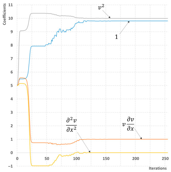
Figure 7.
A process of reconstructing the momentum equation with slip. The library of four possible terms is used. The maximum number of sensors is available.
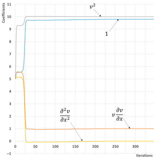
Figure 8.
A process of reconstructing the momentum equation with slip. The library of four possible terms is used. The minimum number of sensors is available.
For a considered library of six possible term candidates, a one-time optimization process does not lead to any reasonable results in all considered cases (See Figure 9 and Figure 10). In particular, for the maximum information scenario, the estimated values of coefficients are c1 = 3.8, c2 = 5.0, c3 = –3.8, c4 = 0, c5 = 2.3, c6 = 9.0, which significantly deviates from the true values. It should be noted, though, that the diffusion term (corresponding to c4) is omitted from the analysis quite efficiently, as in both cases its absolute value is close to zero. Furthermore, supplementing the process with an additional optimization corrects the values of coefficients to the correct values during additional 727 iterations. The obtained values of c1 = 9.8, c2 = 0, c3 = 0, c4 = 0, c5 = 1, c6 = 10. Unfortunately, no meaningful results have been obtained with a single pressure sensor available, despite the increased optimization process.
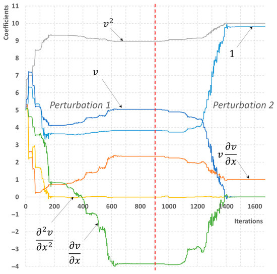
Figure 9.
A process of reconstructing the momentum equation with slip. The library of six possible terms is used. The maximum number of sensors is available.
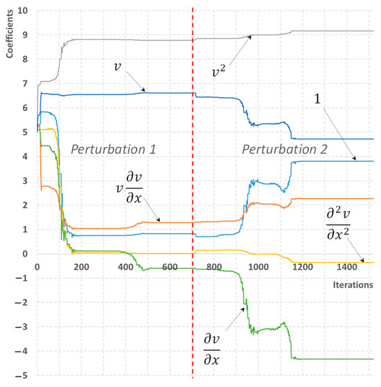
Figure 10.
A process of reconstructing the momentum equation with slip. The library of six possible terms is used. The minimum number of sensors is available.
Therefore, despite more complex physics and advanced algorithms for direct problem solution, the potential of reconstructing the momentum equation with slip remains the same as in the case of homogeneous flow. Though obtaining a quantitatively correct solution may require additional measurements, which can be expressed either in terms of more sensors or prolonged periods of data acquisition from the measurements.
7. Parameter Estimation
From the analysis of the reconstruction algorithm, it is obvious that this process needs to be performed once for a given wellbore. The necessity of any model refinement may appear only if the expected flow regime may change dramatically, which may be the case if, for example, well construction is updated. However, the specific closure parameters of the model obtained may in principle require some refinement, even during regular well operation. This is driven by the fact that closure parameters of the drift-flux model, namely k, C, vd, are not constant and change with the variation of fluid velocities and composition of phases [21]. Therefore, even a decrease of downhole pressure due to natural reservoir depletion will eventually lead to uncertainty in model closure parameters and ultimately make the modelling approach unapplicable, despite the fact that the form of the governing equations remains correct. In that way, the problem of model refinement through additional parameter estimation becomes an important part of the equation reconstruction process. Obviously, this problem becomes even more relevant when the physical model is obtained from physical formulation as such, rather than being reconstructed from data.
One of the available methods to update the parameters of the dynamic model is by using the Kalman filter [27] and its various non-linear variations [28]. It was also applied to the multiphase wellbore flow [29]. However, the filtering approach has certain disadvantages. Firstly, it is the complexity of formulating the filtering problem, especially if the model is given in implicit form. Secondly, it is the recursive nature of the filtering approach, which imposes constraints on the datasets used as an input to the computational algorithm. Alternatively, a variant of the optimization approach used for equation reconstruction can be adapted to the problem of parameter estimation. In this case, the residual R needs to be minimized as a function of model parameters.
A problem of parameter estimation is formulated as follows. It is assumed that the function F in Equation (11) is obtained and corresponds to (18), so that the momentum conservation is accurately described by Equation (5). Then, the remaining sources of uncertainty for the drift-flux model are k, C, vd. Then, the residual in the form of (13) or (14) can be formulated as a function of these three parameters R = R(k, C, vd), with the target values of these three parameters calculated through the optimization approach.
Figure 11, Figure 12, Figure 13 and Figure 14 demonstrate how the model parameters are updated through the optimization process for both homogeneous flow model and a flow with a slip. In both cases regardless the amount of input information used, the correct values of model parameters have been obtained. These equal to k = 10 m−1, C = 1, vd = 0 for homogeneous flow (Figure 11 and Figure 12), and k = 10 m−1, C = 1.2, vd = 0.4 m/s for flow with slip (Figure 13 and Figure 14).
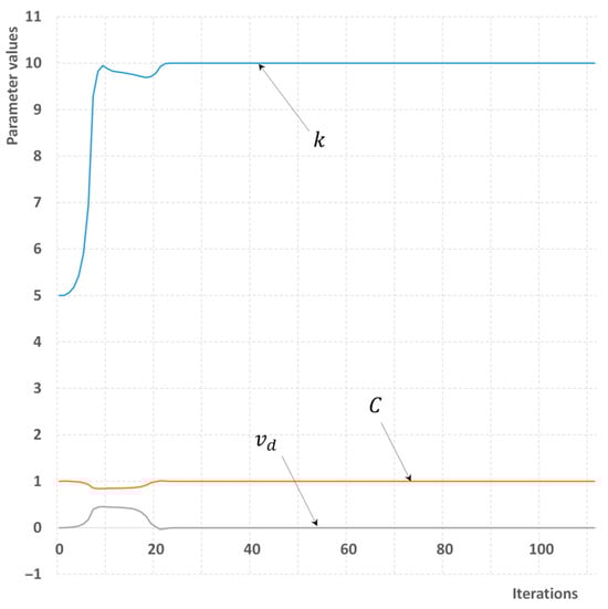
Figure 11.
A process of parameter estimation for homogeneous flow. The maximum number of sensors is available.
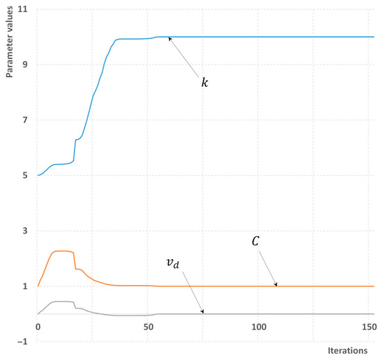
Figure 12.
A process of parameter estimation for homogeneous flow. The minimum number of sensors is available.
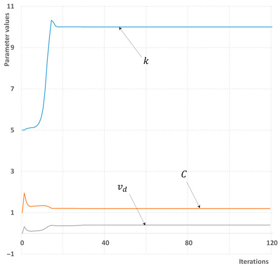
Figure 13.
A process of parameter estimation for the drift-flux model. The maximum number of sensors is available.
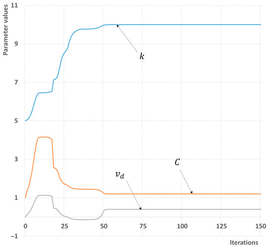
Figure 14.
A process of parameter estimation for the drift-flux model. The minimum number of sensors is available.
It was observed though that with minimum information available, the first 50 iterations are characterized by a significantly overestimated value of drift velocity vd. With the maximum information available, the convergence process ends faster; in particular for homogeneous flow (Figure 11), the correct value of all three parameters is calculated within 20 iterations only. In summary, the problem of parameter estimation through minimization of residual is solved much faster and more accurately in general than a problem of equation reconstruction (Section 5 and Section 6). Also, there is no need for additional flow disturbances. This is explained by the fact that the number of parameters in the optimization domain is reduced and also that the impact of model parameters on the flow field is less than the contribution of certain equation terms, which could qualitatively change the type of the obtained solution. The absolute error of the estimation, that is the difference between the predicted and true values of model parameters, was of order 10−8–10−9 for all considered cases. An example of a source code for the parameter estimation problem is available as a Supplementary Material.
8. Analysis of Sensor Setup
This section presents a brief discussion about the measurement layout used. Firstly, it is important to note that the sensor configuration considered is not specific to any particular wellbore. Rather, it represents two extreme scenarios: firstly, the wellbore is fully instrumented, and secondly, it is poorly equipped. While the former is the preferable case, in reality it is expected to have only a few sensors available, as multiphase flow meters are generally expensive to purchase and maintain. Under such reasoning, it has been investigated what the minimum amount of information is needed in order to unequivocally reconstruct flow equations and estimate the parameters of the drift-flux model. In this respect, the configuration with the only single pressure gauge available may appear insufficient for such tasks. However, from a mathematical perspective, it is the transient nature of flow that facilitates the extraction of additional information from a single pressure reading. This claim is supported by the successful equation reconstruction (Section 5.2 and Section 6.2) and parameter estimation (Section 7) for minimum information scenarios.
It should be noted, though, that the sensitivity of a location of a pressure gauge in a single-sensor scenario has not been properly evaluated. In our understanding, moving this location further downstream from the inflow point will affect the reconstruction process in a negative way. Firstly, this is due to the decrease of the pressure drop between the topside pressure and readings at the gauge. Secondly, the flow disturbance caused by fluid inflow will get distorted due to friction, and the amount of this distortion will strongly be related to the distance between the measurement station and the inflow point. In other words, the further downstream of the inflow point the pressure gauge is located, the worse the results of the estimation will be in a single pressure gauge scenario. A detailed analysis of proper sensor placement will require an exhaustive sensitivity study, and it is an important topic for future work.
When comparing measurement configurations used, one can note that both allow us to obtain proper results in terms of both equation reconstruction and parameter estimation. The essential difference is within the number of interactions required to achieve the convergence, which is significantly less when the wellbore is fully instrumented. In addition, using a single pressure gauge only potentially requires a significant transient wellbore, flow, which is maintained by creating additional disturbance by manipulating a wellhead choke. All these findings can be converted into recommendations for potential wellbore instrumentation and integrated into a field development plan. Financial considerations, stemming from budgeting and capital investments, also influence the specific choice of installed sensors type and number.
9. Conclusions and Future Work
It has been demonstrated that the approach suggested in this work is versatile, and it can easily be applied to an arbitrary problem, which can at least approximately be represented by a system of partial differential and algebraic equations. Then, the equations, which are unknown or known to a certain extent only, can be reconstructed based on the measurements associated with the considered physical process. This methodology should be mainly considered as a tool for physical research, which automates the process of model identification. In this work a complete identification of drift-flux wellbore flow equations has been performed, which could potentially be further used for intelligent production monitoring, such as virtual flow metering. An assessment has been performed for two scenarios, corresponding to a different degree of wellbore instrumentation frequently encountered in real-life applications. As it follows from the examples considered, the proposed method does indeed handle satisfactorily both equation reconstruction and subsequent parameter estimation with the average absolute error of 10−6.
Although the demonstrated results are promising, more work is required before this technology can be deployed for real-life field applications. Firstly, this work has not addressed real-time estimator performance issues in the presence of significant measurement noise and model error. In order to mitigate this, both small-scale laboratory experiments and field testing should be performed. Secondly, only a single mixture momentum has been considered. Thus, investigation into reconstruction of multiple equations (e.g., multi-fluid wellbore model) is another promising area for research. This can be investigated if the multiphase wellbore flow is described in a multi-fluid formalism, which leads to several momentum equations to be reconstructed. Finally, a greater range of operating conditions could be handled by taking the water phase into consideration, as the multiphase wellbore flow is normally three-phase. This would naturally need additional measurements, and the temperature measurements obtained through downhole gauges or distributed sensors are one of the options for such analysis. This would require the energy conservation law to be added to account for temperature variation in flow, which in turn may be subject to equation reconstruction and parameter estimation. All these issues, obviously, are of importance for real-life applications and can become a subject for future research.
Supplementary Materials
The following supporting information can be downloaded at: https://www.mdpi.com/article/10.3390/computation13110253/s1.
Author Contributions
Conceptualization, A.G.; methodology, A.G. and E.M.; software, E.M.; validation, A.G. and E.M.; formal analysis, A.G. and E.M.; investigation, A.G. and E.M.; resources, A.G. and M.A.; data curation, M.A.; writing—original draft preparation, A.G. and E.M.; writing—review and editing, A.G., E.M., and M.A.; visualization, A.G. and E.M.; supervision, A.G.; project administration, M.A. All authors have read and agreed to the published version of the manuscript.
Funding
This research received no external funding.
Data Availability Statement
The original contributions presented in the study are included in the article; further inquiries can be directed to the corresponding author.
Conflicts of Interest
Anton Gryzlov holds the position of Petroleum Engineering Consultant at Aramco Innovations, and Eugene Magadeev holds the position of Research Advisor at SPC. Muhammad Arsalan holds the position of Petroleum Engineering Consultant at Saudi Aramco. The authors declare that the research was conducted in the absence of any commercial or financial relationships that could be construed as a potential conflict of interest.
References
- Sudaryanto, B.; Yortsos, Y.C. Optimization of fluid front dynamics in porous media using rate control. Phys. Fluids 2000, 12, 1656. [Google Scholar] [CrossRef][Green Version]
- Jansen, J.D.; Bosgra, O.H.; van den Hof, P.M.J. Model-based control of multiphase flow in subsurface oil reservoirs. J. Process Control 2008, 18, 846. [Google Scholar] [CrossRef]
- Jansen, J.D. Adjoint-based optimization of multi-phase flow through porous media—A review. Comput. Fluids 2011, 46, 40. [Google Scholar] [CrossRef]
- Nygaard, G.; Nævdal, G. Nonlinear model predictive control scheme for stabilizing annulus pressure during oil well drilling. J. Process Control 2006, 16, 719. [Google Scholar] [CrossRef]
- Santim, C.G.S.; Fulchignoni, L.P.; Rosa, E.S.; Gaspari, E.F. Transient multiphase flow modeling and validation in a real production system with high CO2 content using the drift-flux model. J. Pet. Sci. Eng. 2020, 188, 106903. [Google Scholar] [CrossRef]
- Gouhar, H.; Wenyang, Z.; Youssef, L. Production Assurance of Oil Field by using Integrated Modeling. In Proceedings of the Abu Dhabi International Petroleum Exhibition & Conference, SPE-197713-MS, Abu Dhabi, United Arab Emirates, 11–14 November 2019. [Google Scholar] [CrossRef]
- Leemhuis, A.P.; Nennie, E.D.; Belfroid, S.P.C.; Alberts, G.J.N.; Peters, E.; Joosten, G.J.P. Gas coning control for smart wells using a dynamic coupled well-reservoir simulator. In Proceedings of the SPE Intelligent Energy Conference and Exhibition, SPE-112234-MS, Amsterdam, The Netherlands, 25–27 February 2008. [Google Scholar] [CrossRef]
- Malekzadeh, R.; Belfroid, S.P.C.; Mudde, R.F. Transient drift flux modelling of severe slugging in pipeline-riser systems. Int. J. Multiph. Flow 2012, 46, 32–37. [Google Scholar] [CrossRef]
- Spesivtsev, P.; Sinkov, K.; Sofronov, I.; Zimina, A.; Umnov, A.; Yarullin, R.; Vetrov, D. Predictive model for bottomhole pressure based on machine learning. J. Pet. Sci. Eng. 2018, 166, 825–841. [Google Scholar] [CrossRef]
- Kanin, E.A.; Osiptsov, A.A.; Vainshtein, A.L.; Burnaev, E.V. A predictive model for steady-state multiphase pipe flow: Machine learning on lab data. J. Pet. Sci. Eng. 2019, 180, 727–746. [Google Scholar] [CrossRef]
- Schmidt, M.; Lipson, H. Distilling free-form natural laws from experimental data. Science 2009, 324, 81. [Google Scholar] [CrossRef]
- Ghattas, O.; Willcox, K. Learning physics-based models from data: Perspectives from inverse problems and model reduction. Acta Numer. 2021, 30, 445. [Google Scholar] [CrossRef]
- Haaland, S.E. Simple and explicit formulas for the friction factor in turbulent pipe flow. J. Fluids Eng. 1983, 105, 89. [Google Scholar] [CrossRef]
- Hamdan, M.H. Single-phase flow through porous channels a review of flow models and channel entry conditions. Appl. Math. Comput. 1994, 62, 203. [Google Scholar] [CrossRef]
- Gryzlov, A.; Magadeev, E.; Arsalan, M. A Hybrid Approach for Predictive Control of Oil Well Production Using Dynamic System Identification and Real-Time Parameter Estimation. Computation 2025, 13, 36. [Google Scholar] [CrossRef]
- Jansen, J.-D.; Douma, S.D.; Brouwer, D.R.; Van den Hof, P.M.J.; Bosgra, O.H.; Heemink, A. Closed Loop Reservoir Management. In Proceedings of the SPE Reservoir Simulation Symposium, SPE-119098-MS, The Woodlands, TX, USA, 2–4 February 2009; pp. 856–873. [Google Scholar] [CrossRef]
- Schaeffer, H. Learning partial differential equations via data discovery and sparse optimization. Proc. R. Soc. A 2017, 473, 20160446. [Google Scholar] [CrossRef]
- Brunton, S.L.; Proctor, J.L.; Kutz, J.N. Discovering governing equations from data by sparse identification of nonlinear dynamical systems. Proc. Natl. Acad. Sci. USA 2016, 113, 3932–3937. [Google Scholar] [CrossRef]
- Masella, J.M.; Tran, Q.H.; Ferre, D.; Pauchon, C. Transient simulation of two-phase flows in pipes. Int. J. Multiph. Flow 1998, 24, 739. [Google Scholar] [CrossRef]
- Spesivtsev, P.E.; Kharlashkin, A.D.; Sinkov, K.F. Study of the transient terrain–induced and severe slugging problems by use of the drift–flux model. SPE J. 2017, 22, 1570. [Google Scholar] [CrossRef]
- Shi, H.; Holmes, J.A.; Diaz, L.R.; Durlofsky, L.J.; Aziz, K. Drift-flux parameters for three-phase steady-state flow in wellbores. SPE J. 2005, 10, 130. [Google Scholar] [CrossRef]
- Brinkman, H.C. On the permeability of media consisting of closely packed porous particles. Appl. Sci. Res. A 1947, 1, 81. [Google Scholar] [CrossRef]
- Nocedal, J.; Wright, S.J. Numerical Optimization; Springer: Greer, SC, USA, 2006. [Google Scholar]
- Nelder, J.A.; Mead, R. A Simplex Method for Function Minimization. Comput. J. 1965, 7, 308. [Google Scholar] [CrossRef]
- Patankar, S.V. Numerical Heat Transfer and Fluid Flow; Hemisphere: New York, NY, USA, 1980. [Google Scholar]
- Versteeg, H.K.; Malalasekera, W. An Introduction to Computational Fluid Dynamics the Finite Volume Method; Pearson Education Ltd.: Harlow, UK, 2007. [Google Scholar]
- Kalman, R.E. A new approach to linear filter and prediction problems. J. Basic Eng. 1960, 82, 35. [Google Scholar] [CrossRef]
- Gryzlov, A.; Leskens, M.; Mudde, R.F. A semi-implicit approach for fast parameter estimation by means of the extended Kalman filter. J. Process Control 2011, 21, 510. [Google Scholar] [CrossRef]
- Lorentzen, R.J.; Nævdal, G.; Lage, A.C. Tuning of parameters in a two-phase flow model using an ensemble Kalman filter. Int. J. Multiph. Flow 2003, 29, 1283. [Google Scholar] [CrossRef]
Disclaimer/Publisher’s Note: The statements, opinions and data contained in all publications are solely those of the individual author(s) and contributor(s) and not of MDPI and/or the editor(s). MDPI and/or the editor(s) disclaim responsibility for any injury to people or property resulting from any ideas, methods, instructions or products referred to in the content. |
© 2025 by the authors. Licensee MDPI, Basel, Switzerland. This article is an open access article distributed under the terms and conditions of the Creative Commons Attribution (CC BY) license (https://creativecommons.org/licenses/by/4.0/).