Article

An Analysis of the Computational Complexity and Efficiency of Various Algorithms for Solving a Nonlinear Model of Radon Volumetric Activity with a Fractional Derivative of a Variable Order

Institute of Cosmophysical Research and Radio Wave Propagation FEB RAS, Mirnaya Street 7, Paratunka 684034, Russia
Computation 2025, 13(11), 252; https://doi.org/10.3390/computation13110252
Submission received: 28 September 2025 / Revised: 19 October 2025 / Accepted: 20 October 2025 / Published: 2 November 2025
(This article belongs to the Section Computational Engineering)

Abstract

The article presents a study of the computational complexity and efficiency of various parallel algorithms that implement the numerical solution of the equation in the hereditary α ( t ) -model of radon volumetric activity (RVA) in a storage chamber. As a test example, a problem based on such a model is solved, which is a Cauchy problem for a nonlinear fractional differential equation with a Gerasimov–Caputo derivative of a variable order and variable coefficients. Such equations arise in problems of modeling anomalous RVA variations. Anomalous RVA can be considered one of the short-term precursors to earthquakes as an indicator of geological processes. However, the mechanisms of such anomalies are still poorly understood, and direct observations are impossible. This determines the importance of such mathematical modeling tasks and, therefore, of effective algorithms for their solution. This subsequently allows us to move on to inverse problems based on RVA data, where it is important to choose the most suitable algorithm for solving the direct problem in terms of computational resource costs. An analysis and an evaluation of various algorithms are based on data on the average time taken to solve a test problem in a series of computational experiments. To analyze effectiveness, the acceleration, efficiency, and cost of algorithms are determined, and the efficiency of CPU thread loading is evaluated. The results show that parallel algorithms demonstrate a significant increase in calculation speed compared to sequential analogs; hybrid parallel CPU–GPU algorithms provide a significant performance advantage when solving computationally complex problems, and it is possible to determine the optimal number of CPU threads for calculations. For sequential and parallel algorithms implementing numerical solutions, asymptotic complexity estimates are given, showing that, for most of the proposed algorithm implementations, the complexity tends to be n 2 in terms of both computation time and memory consumption.

1. Introduction

1.1. Object of Research

Modern science pays close attention to fundamental areas that have practical applications. Much attention is devoted to the mathematical modeling of processes in saturated media in economics, biology, geophysics, seismology, and other fields. For the Kamchatka region, the problem of seismicity is ascribed the highest priority since the Kamchatka Peninsula is located in one of the most seismically dangerous areas on Earth, and strong earthquakes, such as the recent one on 30 July 2025 with a magnitude of 8.8, can cause enormous damage. This determines the importance of research that contributes to a deeper understanding of the processes occurring in the Earth’s crust in preparation for a future earthquake, with the aim of creating a more effective forecasting system in the future. The study of subsoil gas migration processes using the most advanced mathematical modeling methods to interpret anomalies preceding earthquakes is a new and relevant research method in geophysics.
Monitoring changes in the concentration of radioactive radon gas ( Rn 222 ) in subsoil and atmospheric air [1] and water [2] is considered a well-known and well-established indicator of processes occurring in the geological environment, especially as a short-term precursor (up to 15 days), as shown in the works [3,4] and many others. Omitting details related to monitoring, research on Rn 222 as a precursor, and the modeling of various processes, which can be found in [5,6,7] and others, we will note only two things. Firstly, experimental data is measured using a device with a gas discharge counter for Rn 222 in an accumulation chamber, so, when we talk about radon, we mean the volume activity of radon (RVA) in the accumulation chamber, or, more precisely, variations in RVA over time. Secondly, the mass transfer process of Rn 222 is non-local in nature. Therefore, there are often cases when radon exhibits unusual migration capabilities [8], and it is impossible to explain this using only the diffusion mechanism described by ordinary derivatives or the convection (advection) mechanism. However, if we consider the geological environment as a medium with a complex topology, heterogeneous and porous, in a word, fractal [9], then the process transfer Rn 222 can be considered from the perspective of anomalous transfer processes [10].
Therefore, the authors in studies [11,12] propose mathematical hereditary models of RVA, but taking into account non-locality in time, which leads to the heredity effect [13] in the dynamics of Rn 222 transfer [14]. Heredity is the property of a system or environment to remember for some time the impact exerted on it. Heredity is equivalent to such concepts as aftereffect, heredity, residuality, memory and delay, and non-locality. The mathematical apparatus of these models is based on fractional calculus, the theory of which has been studied quite well [15,16,17]. Generalizing known mathematical models and developing new ones that take heredity into account allows us to significantly refine known results [18,19]. In hereditary RVA models, operators of the Gerasimov–Caputo type [20,21] are considered fractional derivatives in hereditary RVA models, both as variable 0 < α ( t ) < 1 -order and constant 0 < α < 1 -order in special cases. Fractal calculus is interrelated with fractal theory, as reflected in the work [9]; in particular, there is a connection between the fractal (Hausdorff) dimension of the medium and the orders of fractional operators. In turn, the orders of fractional operators are related to the concept of heredity—the property of a system or process to retain memory of its past. The main hypothesis of hereditary RVA models is that the order of the fractional derivative is related to the transport intensity Rn 222 and, therefore, to the change in the permeability of the geological medium due to changes in the stress–strain state of the medium.
The proposed RVA models have been validated using experimental data from Rn 222 monitoring stations at the Petropavlovsk–Kamchatsky geodynamic test site and Sakhalin Island. It is shown in [11] that the hereditary α -model RVA can well describe not only accumulation processes with a certain choice of parameters but also decay processes. Also, in [11,12] shows that the hereditary α ( t ) -model RVA can describe complex impulses (bursts) due to a specific type of functions included in the model equations (Figure 1). The identification of the signs of such processes in radon observation data is one of the pressing tasks in geophysics.

1.2. Theoretical and Practical Significance of the Research

Fractional differential equations can be used in problems involving the modeling of anomalous variations in RVA in an accumulation chamber. Anomalous variations in radon gas monitoring data are considered short-term precursors of earthquakes and indicators of geological processes. However, the mechanisms behind such anomalies are still poorly understood, and direct observations are impossible. This highlights the importance of mathematical modeling and effective algorithms for solving such problems. This subsequently allows us to move on to inverse problems based on monitoring data, for which it is important to select the most suitable algorithm for solving the direct problem. But in the studies mentioned by the authors, all parameters of the RVA models were selected manually by comparing the solution with the processed experimental data and visual assessments of the degree of similarity [22] using R 2 —the coefficient of determination, and R—Pearson’s correlation coefficient. This logically leads to the search for solutions for automating the selection. The need to automate the selection of model parameters often arises when working with geological data, in geophysics and seismology, etc., since it is impossible to take direct measurements of these parameters [23].
Therefore, in their works [24,25], the authors formulate and solve the inverse problem [26,27,28] to restore the parameter values in the hereditary α -model RVA, and in [29,30] to restore the values and form of the function α ( t ) in the hereditary α ( t ) -model RVA. In [25], a hereditary mathematical model was applied for the first time to estimate the change in radon flux density (RFD) based on the solution of the inverse problem when the stress–strain state of the medium changed before and after a strong earthquake in Kamchatka on 17 August 2024. The simulation results obtained are given a physical interpretation, and the estimates are reliable and more accurate than for the other RVA model. The practical significance of the RFD assessment results using hereditary mathematical RVA models is that they can help in the more accurate selection of locations for Rn 222 monitoring stations.
To solve inverse problems, the authors use the Levenberg-Marquardt iterative method [31], which requires a cyclical recalculation of the solution to the direct problem for different values of the parameters of the RVA hereditary model and comparison of the results with experimental data. However, the convergence rate of the recovered values to the optimal ones is unknown in advance. At the same time, the direct problem can have a sufficiently high computational complexity both when increasing the size of the input data, N and when choosing the solution method. For example, when the sampling frequency of the experimental RVA data changes, the number, N, of nodes in the grid of the numerical method for solving the direct problem will increase by several tens of times. Therefore, it is important that the solution of each individual direct problem is calculated in the shortest possible time, but simultaneously, it is necessary to take into account the possible memory costs of the algorithm used. All of this leads us to the development of various parallel algorithms for the numerical solution of RVA model equations, the analysis of their efficiency, and estimates of computational complexity.

1.3. Subject of Research

This study considers parallel implementations of numerical solution methods: EFDS (non-local explicit finite difference scheme) and IFDS-MNM (non-local implicit finite difference scheme solved by a modified Newton method) with the aim of estimating the computational complexity and efficiency of these algorithms.
In article [32], the authors present a parallel hybrid implementation of EFDS on a GPU and provide performance estimates, but on a different test example for a personal supercomputer. The acceleration of calculations is achieved by pre-computing the values of all parameters and functions on the computational grid. It is shown that EFDS has an unavoidable sequential part in the algorithm, which, as N increases, makes parallel EFDS algorithms not efficient. In turn, IFDS-MNM [33] is solved through an iterative method, which, on the contrary, makes the parallel implementation of IFDS-MNM more efficient than parallel EFDS for a large N.
From [33], it is important to note that EFDS converges with order O ( τ ) and it is stable only under the condition h ( 2 1 max i ( α i ) 1 ) / ( max i ( b i ) ) , which limits its scope of application depending on the h discretization step and the constraints on min ( b i ) , max ( b i ) , and min ( α i ) , max ( α i ) values of the model coefficients when using EFDS. In turn, IFDS-MNM is definitely stable with a convergence order of O h 2 max i ( α i ) and, therefore, does not involve such significant restrictions on model parameters.
As for studies similar to the one presented here, articles [34,35,36] explore issues of accelerating calculations when modeling certain diffusion processes based on a non-local fractional derivative of the Gerasimov–Caputo type and some of its subtypes. The authors propose reducing computational accuracy at the stage of constructing the fractional derivative approximation in order to accelerate the process. It is proposed to solve the model equation numerically, using finite difference schemes. The schemes proposed in [35,36] are implemented as parallel algorithms for systems with PRAM on CPU. In [34], the schemes are implemented on GPUs (graphics accelerators). It is shown that using such approaches can significantly speed up the calculation.

1.4. Article Structure

Section 1 is an introduction describing the object, subject, and practical significance of this study. Section 2 provides a test example based on the hereditary α ( t ) model of RVA. Section 3 discusses the numerical schemes EFDS and IFDS-MNM, as well as block diagrams of their sequential algorithms. Section 4 describes the methodology for measuring the average computation time of different algorithms, as well as the memory consumption of the computing device, and introduces parameters for a concise description of the computation time and memory consumption of different algorithms. Section 5 presents a method for obtaining execution time and memory consumption functions based on experimental data and describes a method for obtaining asymptotically exact complexity estimates. Estimates of the complexity of sequential algorithms are given. Section 6 presents various parallel hybrid CPU–GPU algorithms EFDS-hybrid and IFDS-MNM-hybrid, parallel CPU algorithms EFDS-omp and IFDS-MNM-omp, as well as their block diagrams. Section 7 describes a method for analyzing the efficiency of parallel algorithms and presents results for all four algorithms discussed. Section 8 provides asymptotically exact complexity estimates for all four parallel algorithms in terms of both computation time and memory consumption. Section 9 summarizes the results of the study.

2. Test Example

In this study of computational complexity and algorithm efficiency for solving direct problems, we will consider the hereditary α ( t ) -model RVA from [11] as a test example for describing the anomalous impulse (burst) RVA. This article does not address the goal of the mathematical modeling of RVA variations; only the time from the start to the end of the model calculation is important. Therefore, to simplify the work, we will not specify the dimensions of the parameters and members of the hereditary α ( t ) -model RVA. The model represents a Cauchy problem of the following form:
0 , t α ( t ) A ¯ ( t ) = a ( t ) A ¯ ( t ) 2 b ( t ) A ¯ ( t ) + c ( t ) , A ¯ ( t ) = A ( t ) A m a x , A ¯ ( t 0 ) = A 0 A m a x ,
where
  • A ¯ ( t ) —RVA in dimensionless form;
  • A ( t ) —RVA, A m a x —maximum RVA value observed in the data; A 0 —RVA at the initial moment in time;
  • t [ t 0 , T ] —time of the process under consideration; t 0 and T > 0 —initial and final moments in time;
  • a ( t ) —a function, like the member it stands for, related to the output Rn 222 from the chamber into the surrounding atmosphere at a pressure difference between the internal (chamber) and atmospheric pressures, for example, when passing in the vicinity of a cyclone observation point;
  • b ( t ) = λ 0 —the air exchange rate;
  • c ( t ) —a function describing the diffusion mechanism of Rn 222 transport into the chamber [37];
  • 0 , t α ( t ) A ¯ ( t ) —a model member describing the delay associated with time non-locality in the process of transport Rn 222 through the geological environment.
Time delay in the model (1), according to [11,12], is described by a fractional differentiation operator of the Gerasimov–Caputo type [20,21] of variable order 0 < α ( t ) < 1 of the form: 0 , t α ( t ) A ¯ ( t ) = 1 Γ ( 1 α ( t ) ) 0 t A ¯ ˙ ( τ ) d τ ( t τ ) α ( t ) , where Γ () is Euler’s gamma function.
Example 1.
Let us consider the problem (1) with the following parameter values:
T = 22 , A ¯ = 0 , A ¯ m a x = 1 , λ 0 = 0.05 , θ = 1 , α ( t ) = 0.99 1 ( T t ) T cos 3 π t T 2 , b ( t ) = λ 0 , a ( t ) = 2 λ 0 + 12 λ 0 2 cos π t T 2 + cos 2 π t T π 11 2 , c ( t ) = 12 λ 0 12 ( T t ) 10 T sin 2 π t T 2 + ( T t ) T sin 3 π t T 2 .
The Cauchy problem (1) at (2) is solved numerically since the model equation in (1) is nonlinear and fractional-differential [38]. For this purpose, the authors in [33] proposed the following: EFDS (non-local explicit finite difference scheme) and IFDS-MNM (implicit finite difference scheme solved through the modified Newton method). Regardless of the scheme, the numerical solution is considered in a uniform mesh domain, Ω ^ :
h = T / N , Ω ^ = ( t i = i h ) : 0 i < N , A ¯ ( t ) = A ¯ i , 0 < A ¯ i < 1 , a ( t ) = a i , c ( t ) = c i , α ( t ) = α i .
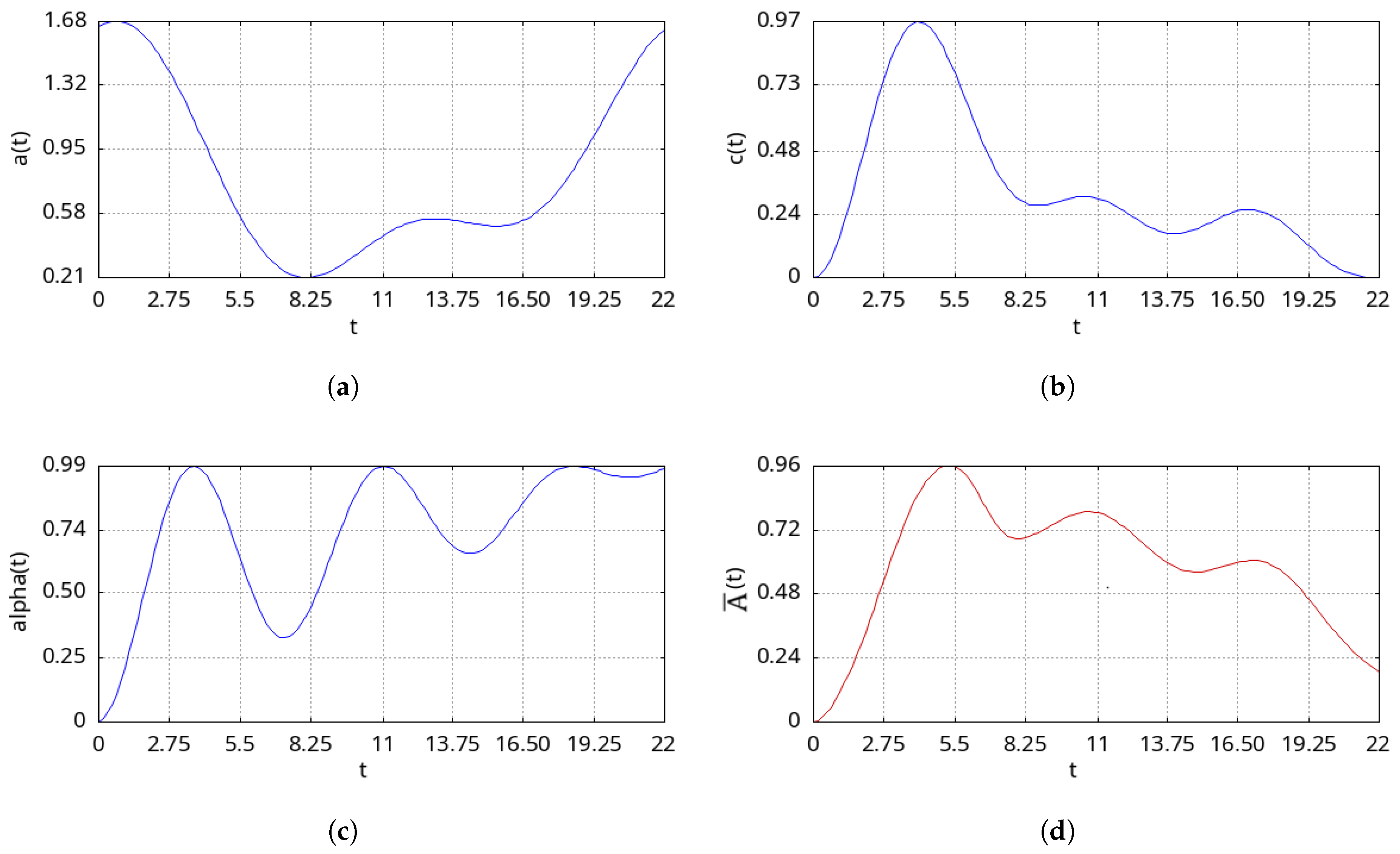
The difference between the example under consideration is that, in this study, we will obtain solutions to the test problem for different values of N, multiples of 100, instead of N = 132 , as in the work [11] (see Figure 1). This is done for clarity, to simplify the construction of graphs, and to simplify the work with estimates. The results of solving the direct problem for IFDS-MNM are shown in (Figure 2), and the result for EFDS will be similar.
This test example was chosen for two reasons. First, this problem was not synthesized specifically to analyze the efficiency of the algorithm, but it is significant from the point of view of applied mathematics. Second, the task can have a rather high computational complexity when N increases several dozen times. In this case, the solution presented in (Figure 2 will not change significantly; only the accuracy of the solution will increase as the density of the lattice nodes (3) increases.

3. Sequential Algorithms for Numerical Solutions

The nonlinear equation in (1) can be solved numerically [33] on a uniform grid (3) using the EFDS scheme as follows:
A 1 = 1 D 0 D 0 ( 1 w 1 0 ) + b 0 u 0 a 0 A ¯ 0 2 + c 0 , A 2 = 1 D 1 D 1 1 w 1 1 + b 1 A ¯ 1 + D 1 w 1 1 A ¯ 0 a 1 A ¯ 1 2 + c 1 , A i + 1 = 1 D i D i 1 w 1 i + b i A ¯ i + D i w 1 i A ¯ i 1 D i j = 2 i w j i A ¯ i j + 1 A ¯ i j a i A ¯ i 2 + b i A ¯ i + c i , D i = h α i + 1 Γ ( 2 α i + 1 ) , w j i = ( j + 1 ) 1 α i + 1 j 1 α i + 1 , w 1 i = i = 0 N 1 2 1 α i + 1 1 1 α i + 1 ,
where A ¯ 0 = C is a known constant, the initial condition of the Cauchy problem.
The nonlinear equation in (1) can be solved numerically [33] on a uniform grid (3) using the IFDS scheme as follows:
D i j = 0 i 1 w j i A ¯ i j A ¯ i j 1 = a i A i ¯ 2 b i A i ¯ + c i , A 0 ¯ = C , D i = h α i Γ ( 2 α i ) , w j i = ( j + 1 ) 1 α i j 1 α i , 1 i < N ,
where A ¯ 0 = C is a known constant, the initial condition of the Cauchy problem.
The IFDS scheme (5) and its generalized analogs have been verified in a series of test and applied problems [11,33], where solutions of the IFDS scheme (5) are considered both as a modified Newton method (MNM) and as Newton’s method.
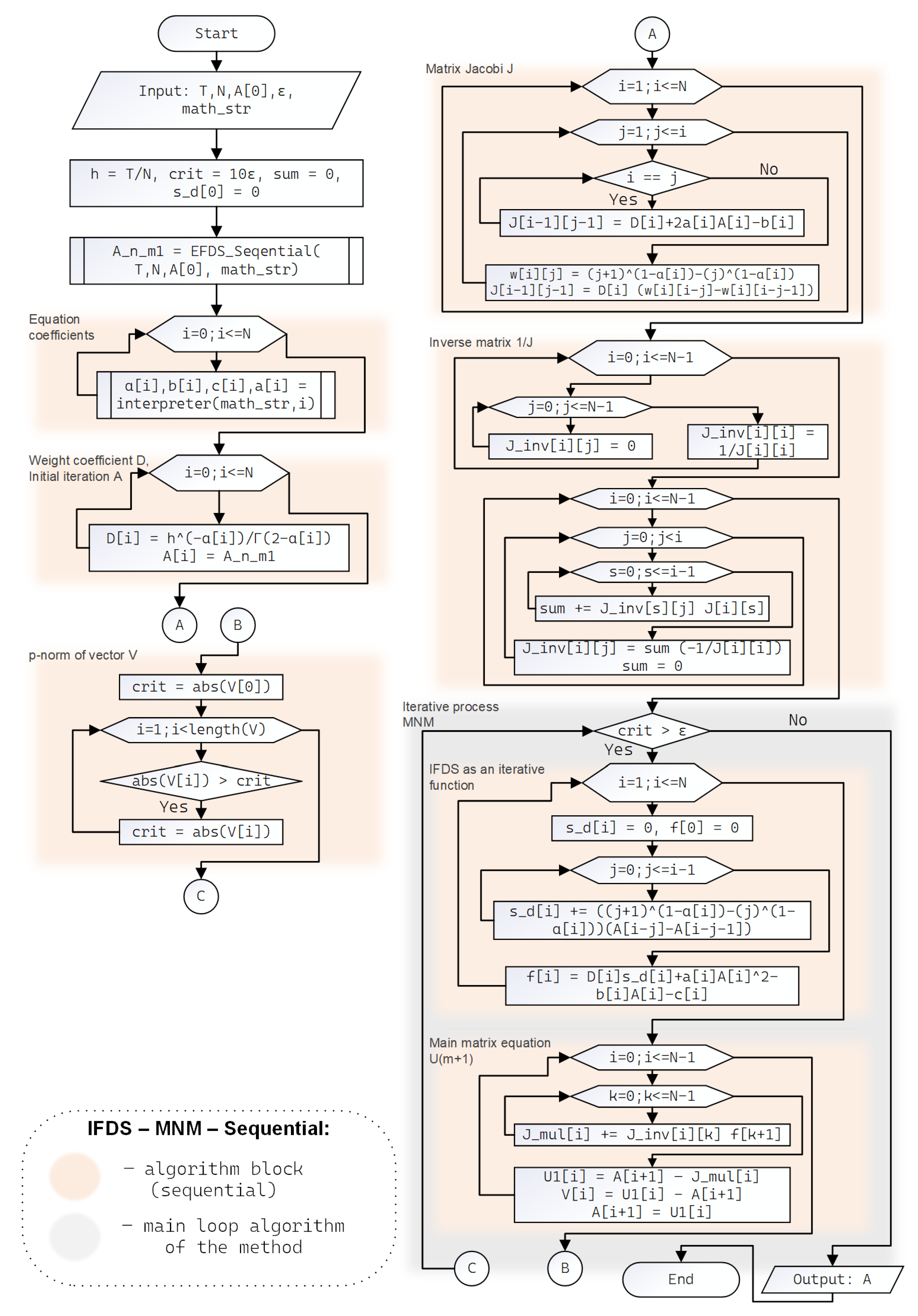
MNM begins by presenting the scheme (5) as an iterative function:
F A i ¯ = D i j = 0 i 1 w j i A ¯ i j A ¯ i j 1 + a i A i ¯ 2 + b i A i ¯ c i ,
and for the iterative function (6), the iterative process is formed:
U m + 1 = U m F U m J U m ,
where m is the iteration step; U m = A ¯ 1 m , , A ¯ N m T is the vector of solution function values at all grid nodes i = 1 , , N known at the iterative m (current) step; F U m = f 1 A ¯ 1 m , , f N A ¯ N m are values calculated according to (6), taking into account the values U m of the solution at step m, and J U m = J i j , i = 1 , , N , j = 1 , , N is Jacobian, the lower triangular matrix, calculated using the formula [33]:
J i j = 0 , j i + 1 , D i b i + 2 a i A ¯ i , j = i , D i w i j i w i j 1 i , j i 1 .
The iterative solution method will not work if there is a singularity at zero for the iterative function of the method (6). To eliminate this, as an initial approximation, U 0 , a vector can be constructed from the value A ¯ N 1 obtained when solving the problem using EFDS (Figure 3). In other cases, a vector is constructed from A ¯ 0 values.
The process continues until the specified solution accuracy, ε , is reached. The criterion for exiting the cycle will be G, the difference between the new solution obtained and the current one, such that G ε , where G = max i U m + 1 U m .
MNM differs from Newton’s method only in that (8) is calculated once, before the start of the iterative process. This will increase m, the number of iterations for the convergence of the method, but it will reduce the total running time of the algorithm (Figure 4), since the computationally complex task of inversion (8) is performed only once.

4. Average Execution Time Using Different Algorithms

We will analyze and evaluate parallel algorithms based on data on the execution time of various programming implementations of EFDS (4) and IFDS-MNM (5). The terms ‘number of algorithm operations’ and ‘computational complexity of the algorithm’ [39,40] are sometimes used as synonyms for the concept of algorithm execution time. All calculations in this article were performed on a computer with the following specifications: CPU—AMD Ryzen 9 7950X, 16 × 4.5 GHz core, cache L2 16 Mb and L3 64 Mb, RAM—96 Gb; GPU—GeForce RTX 4090, 24 Gb, 2235 MHz, and ALU 16384.
The EFDS and IFDS-MNM programming implementations are integrated into the FEVO v1.0 software package, which was developed as part of a grant entitled ‘Development of a software package for modeling and analyzing radon volumetric activity as a precursor to strong earthquakes in Kamchatka to solve direct and inverse problems in RVA dynamics modeling. Among other things, FEVO v1.0 implements an interpreter of user-entered mathematical expressions for specifying the functional dependencies of coefficients and parameters of hereditary models. Using the interpreter to calculate the vectors of coefficient values and parameters of the test problem (2) slightly slows down the initial stage of all EFDS and IFDS-MNM algorithms.
From the lemma of a Brent [41,42,43], it follows that any algorithm implemented for execution in systems with shared memory, such as parallel random-access memory (PRAM), multi-threaded CPU, and control devices, can be modified so that it can be executed in PRAM systems with fewer CPU threads. In other words, we can compare the execution time of algorithms on systems with a single thread (sequential) and different numbers of threads (parallel). Moreover, some algorithms perform part of the calculations on the GPU.
Remark 1.
Since we will obtain a little different results for T—execution time in [sec.], then, with each new numerical experiment, and the number of experiments being finite, T can be considered a random value with a certain distribution function. Then, to calculate T, we will resort to the concept of mathematical expectation [22] for a discrete random value:
T p , g ( N ) = 1 L i = 1 L T p , g i ( N ) ,
where i is the experiment index, L is the sample size, p is the number of CPU threads, g is the number of GPU multiprocessors, and N is the number of nodes (3), i.e., the size of the input data.
Next, for estimates of ‘time complexity’, according to (9) and a sample of L = 10 values, we will use the following parameters in [sec.]:
  • T 1 , 0 ( N ) —the execution time of a test example of size N spent by sequential (EFDS, IFDS-MNM) algorithms;
  • T p , 0 ( N ) —the execution time of a test example of size N spent by parallel (EFDS-omp, IFDS-MNM-omp) algorithms based on the OpenMP API [44], on a machine with p 2 CPU threads;
  • T p , g ( N ) —the execution time of a test example of size N spent by hybrid parallel (EFDS-hybrid, IFDS-MNM-hybrid) algorithms based on the OpenMP API and CUDA API [45,46] on a machine with p 2 CPU threads and a certain fixed number, g.
The user cannot control the number of GPU multiprocessors that will be used for calculations within the FEVO v1.0 software complex but can change the number of thread per block, depending on the specific GPU architecture. All algorithms mentioned in the article are integrated into FEVO v1.0. This includes functions that calculate the optimal (most productive) grid for utilizing CUDA GPU cores based on a specified number of thread. The default setting is thread = 32. As practice shows, changing the number of thread will not significantly change the execution time with a different grid configuration, but when calculating with thread = 32, ‘artifacts’ are excluded, i.e., errors caused by incorrect grid configuration for the parts of the algorithm executed on the GPU.
Similarly, for estimates of ‘memory complexity,’ the concept of M—memory used (RAM) in [Mb]—is employed, and the following parameters are introduced:
  • M 1 , 0 ( N ) —RAM usage when executing a test example of size N using sequential (EFDS, IFDS-MNM) algorithms;
  • M p , 0 ( N ) —RAM usage when executing a test example of size N using parallel (EFDS-omp, IFDS-MNM-omp) algorithms;
  • M p , g C ( N ) —RAM usage when executing a test example of size N using hybrid parallel (EFDS-hybrid, IFDS-MNM-hybrid) algorithms on a machine with p 2 CPU threads and a fixed number g;
  • M p , g G ( N ) —similarly, the use of node GPU memory when executing a test example of size N using hybrid parallel (EFDS-hybrid, IFDS-MNM-hybrid) algorithms.

5. Complexity Estimates for Sequential Algorithms

In computational theory, there is a concept known as ‘algorithm complexity’—an indicator of the amount of resources required for an algorithm, depending on the size of its input data. A distinction is made between time complexity—the relationship between the amount of input data N and the number of elementary operations or the time required to execute all operations of the algorithm—and space complexity, the amount of memory that the algorithm uses to store data during execution. Both types of algorithm complexity are usually expressed as a function of N and evaluated in asymptotic notation. In our case, the first is the parameter T—the average ‘algorithm execution time’ in [sec.], expressed below as the T function, and the second is the parameter M—‘memory complexity’, i.e., the RAM used by a certain computing node in [Mb], expressed below as the M function.
Remark 2.
Analyzing the efficiency of algorithms using such T -functions can be rather difficult, for example, when such a function has a large number of local extremum points, or when a situation arises where the execution time of the algorithm on input arrays with odd lengths is greater than the execution time on arrays with even lengths. Therefore, asymptotic bounds (estimates) of execution time are used in the theory of computational complexity of algorithms [39]. To obtain a Θ-asymptotically exact estimate of complexity, it is necessary to show that:
Θ ( f p , g ( N ) ) = T p , g ( N ) : k 1 > 0 , k 2 > 0 , N 0 0 , 1 , 2 , , 0 k 1 f p , g ( N ) T p , g ( N ) k 2 f p , g ( N ) , N N 0 ,
which is also true for M -functions.
Now, let us conduct a series of computational experiments on sequential algorithms EFDS (Figure 3) and IFDS-MNM (Figure 4), varying the size of the input data N and obtaining data for T, and we will present the results in (Table 1).
Now, having information about the execution time of sequential EFDS and IFDS-MNM algorithms, depending on the size N (Table 1), to estimate the ‘time complexity’ using polynomial interpolation, we can construct T —the algorithm execution time function. In this case, T is an n-degree polynomial, and the order of growth of the execution time function is determined by its highest f p , g ( N ) -dominant member [39].
Using MATLAB, R2024b in particular the polyfit() function, we get the next polynomials:
T 1 , 0 E F D S ( N ) = 0.16028 n 12.51764 , T 1 , 0 I F D S M N M ( N ) = 0.000004 n 2 0.004518 n + 1.077855 ,
and the results are presented in (Figure 5). The quality of the polynomials approximation of the data (Table 1) is measured with the R 2 coefficient of determination.
Indeed, for (11), the inequalities (10) hold under the following conditions:
Θ ( n ) = T 1 , 0 E F D S ( N ) = Q n 12.51764 , Q = 0.16028 , k 1 = 0 , k 2 > Q , N 78 ,
Θ ( n 2 ) = T 1 , 0 I F D S M N M ( N ) = Q n 2 0.004518 n + 1.077855 , Q = 0.000004 , k 1 = 0 , k 2 > Q , N 749 ,
where Q indicates the coefficient of the highest degree of the polynomial, which means that the execution time function with the sequential algorithm T 1 , 0 ( N ) is asymptotically bounded from below and above by the polynomial function f p , g ( N ) with an accuracy of a constant k 2 . In other words,
  • For the sequential EFDS algorithm, the asymptotically exact estimate of time complexity is of the order of Θ ( n ) ;
  • For the sequential IFDS-MNM algorithm, the asymptotically exact estimate of time complexity is of the order of Θ ( n 2 ) .
A similar logic applies to the ’memory complexity’ and M —the function of memory usage for the algorithm (Figure 6). As a result, we obtain the following polynomials:
M 1 , 0 E F D S ( N ) = 0.030517 n + 0.000205 , M 1 , 0 I F D S M N M ( N ) = 0.05722 n 2 + 0.724487 n + 0.002083 ,
and for (13), the inequalities (10) hold under the following conditions:
Θ ( n ) = M 1 , 0 E F D S ( N ) = Q n + 0.000205 , Q = 0.030517 , k 1 = 0 , k 2 > Q , N 1 ,
Θ ( n 2 ) = M 1 , 0 I F D S M N M ( N ) = Q n 2 + 0.724487 n + 0.002083 , Q = 0.05722 , k 1 = 0 , k 2 > 13.69 Q , N 1 ,
In other words,
  • For the sequential EFDS algorithm, the asymptotically exact estimate of memory complexity is of the order of Θ ( n ) ;
  • For the sequential IFDS-MNM algorithm, the asymptotically exact estimate of memory complexity is of the order of Θ ( n 2 ) .
Figure 6. Results for memory usage, as well as the M function interpolating the data (Table 2): (a) EFDS; (b) IFDS-MNM.
Computation 13 00252 g006
Remark 3.
One sequential algorithm is considered more efficient compared to another if its time function, T 1 , 0 ( N ) , exhibits a lower order of growth as N increases. However, in algorithms implementing numerical methods, accuracy and stability are at least as important as their time efficiency or memory cost optimality. As shown above, the sequential EFDS algorithm has a growth order of Θ ( n ) , while the sequential IFDS-MNM algorithm has Θ ( n 2 ) . Although the use of EFDS is preferable, the EFDS numerical scheme involves significant drawbacks compared to IFDS-MNM.
In particular, as shown in the study [33], the EFDS method converges with order O ( τ ) and is stable only under the condition h ( 2 1 max i ( α i ) 1 ) / ( max i ( b i ) ) , which limits its applicability, depending on the discretization step h and the constraints on min ( b i ) , max ( b i ) , as well as min ( α i ) , max ( α i ) values of the model coefficients. This becomes critical when solving inverse problems, for which model coefficients are adjusted through repeated resolution of the direct problem, and due to this limitation, the EFDS method may fail to reach the global optimum.
In turn, IFDS-MNM is undoubtedly stable with a convergence order of O h 2 max i ( α i ) and therefore does not involve such significant restrictions on the model parameters. Although IFDS-MNM has a higher complexity growth order of Θ ( n 2 ) , as shown above, in most cases, using IFDS-MNM is more reliable. All of this leads us to the development of various parallel implementations of numerical methods.

6. Parallel Algorithms EFDS and IFDS-MNM

To reduce the execution time of EFDS through its various implementations, an important aspect is the preliminary parallel computation of all possible values of functions, parameters, and weighting coefficients that do not depend on the sequential parts of the algorithms. This is done in order to get as much acceleration as possible and the least losses during parallelization, i.e., to obtain algorithms with the best efficiency. In the case of IFDS-MNM, a preliminary parallel computation is also performed for all values that can be calculated before the start of the main iterative algorithm. The iterative solution method itself is well suited for parallelization, both on CPUs and GPUs.
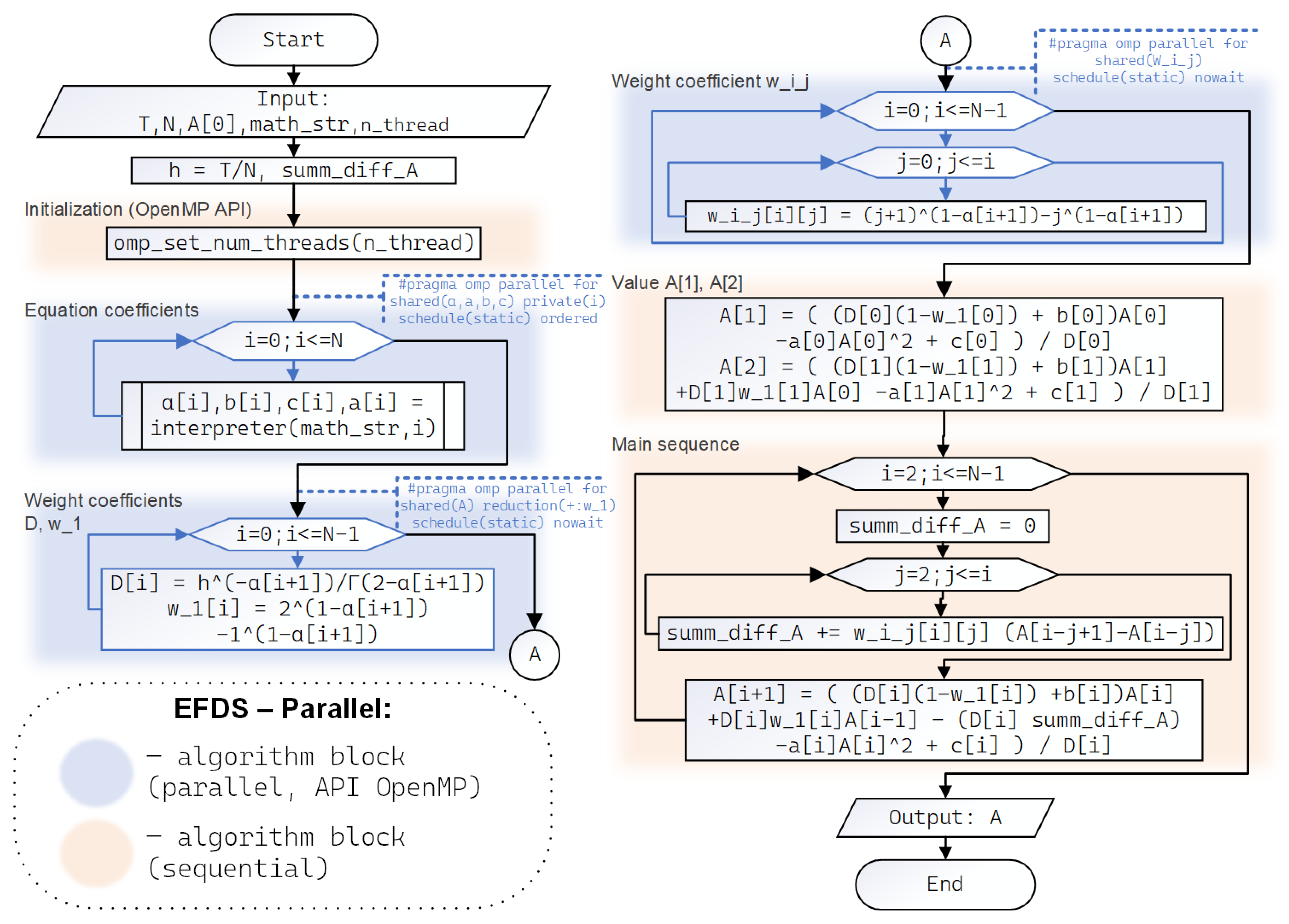
For parallel programming implementation of numerical solution algorithms, the OpenMP API is used—an open software interface standard for parallel systems with shared memory [41,44]. OpenMP is a set of directives for compilers, libraries of functions, and environment variables, and it implements parallel computing using the idea of multithreading—multiple parallel tasks performed using CPU threads. Examples of these algorithms in the form of flowcharts can be seen below: for EFDS-omp (Figure 7) and for IFDS-MNM-omp (Figure 8).
Remark 4.
As the primary programming language (specifically for implementing numerical solution algorithms) in the FEVO v1.0 software package, the C language according to the C99 standard was chosen due to its versatility [47] and extensive capabilities for memory management through the concept of pointers [48].
To work with the GPU, NVIDIA’s CUDA parallel computing API is used, which allows you to manage GPU RAM at your discretion. GPU memory has a hierarchical structure and is optimized for maximum throughput [45,46]. Since the main language is C, the pseudo-code in the flowcharts (Figure 9 and Figure 10) contains code fragments in the C language and its CUDA add-ons. Some trivial operations are not listed in the flowchart, for example, function calls: cudaMalloc()—to allocate GPU RAM, most of the calls cudaFree()—to free GPU RAM, except for those that are important when organizing calculations, as well as the output of results a ( t ) ,   b ( t ) ,   c ( t ) ,   α ( t ) after the main loop.
When implementing EFDS-hybrid algorithms (Figure 9) and for IFDS-MNM-hybrid (Figure 10), an important point is the organization of work with GPU RAM in such a way as to reduce the number of copy operations between CPU RAM and GPU RAM to the required minimum. For example, calculating the values of the function α ( t ) on the entire grid of N nodes on the GPU and storing this data in GPU RAM until the final result is obtained. Below are flowcharts representing the parallelization of numerical solution algorithms using the OpenMP API and the CUDA API.
More information about the nuances of implementing such algorithms in the code and memory management of the GPU, using the example of the EFDS-hybrid algorithm (Figure 9), can be found in [32].

7. Analysis of Efficiency and Optimal CPU Usage for Parallel Algorithms

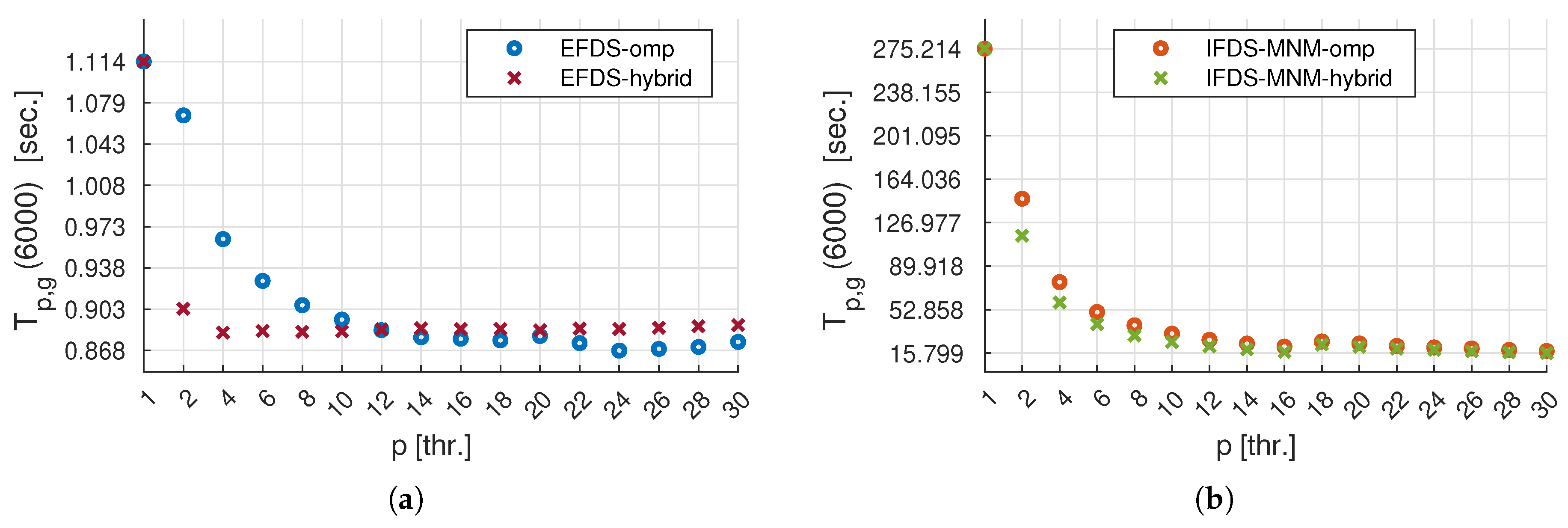
To study the Efficiency of the above parallel implementations of the EFDS and IFDS-MNM algorithms, we will conduct a series of computational experiments for a test example at N = 6000 , but changing the number of CPU threads used p in [units.] in increments of 2. For T p , g ( N ) , the average execution time (9) is also taken as the mean over 10 recalculations. In (Table 3 and Table 4) (Figure 11) the results of computational experiments are presented.
Remark 5.
Algorithm efficiency is the optimal ratio expressed in the coordinates: computation speedup versus the number of computational node threads [41], compared to the most efficient sequential version of the algorithm.
For the analysis of efficiency, data (Table 3) obtained using Formula (9) with L = 10 are used. To evaluate efficiency, the data on T p , g ( N ) are considered in terms of (TAECO), applicable to algorithms: T execution time, A acceleration (speedup), E efficiency, C cost, and O cost-optimal indicator. The results are presented below in (Figure 12) for parallel EFDS and in (Figure 13) for parallel IFDS-MNM.
  • A p , g ( N ) is the acceleration in [unit] that the parallel version of the algorithm provides in comparison with the sequential one and is calculated as follows:
    A p , g ( N ) = T 1 , 0 ( N ) / T p , g ( N ) ,
    where max A p , 0 ( N ) = p is the theoretical case, provided that there are no delays in parallelization for the task before it is sent to different CPU threads for calculation.
  • E p , g ( N ) is the efficiency, in [units/thr.], of using a given number of p CPU threads and is determined via the following ratio:
    E p , g ( N ) = T 1 , 0 ( N ) p · T p , g ( N ) = A p , g ( N ) / p ,
    where, for max A p , g ( N ) = p , we get that max V p , g ( N ) = 1 .
  • C p , g ( N ) is the cost in [sec. × thr.], which is determined by the product of a given number of p CPU threads and T execution time of the parallel algorithm. The cost is determined by the following ratio:
    C p , g ( N ) = p · T p , g ( N ) .
  • O p , g ( N ) is the cost-optimal indicator in [units. × thr.], is characterized by a cost proportional to the complexity of the most efficient sequential algorithm [49] and is calculated as follows:
    O p , g ( N ) = C p , g ( N ) / T 1 , 0 ( N ) .
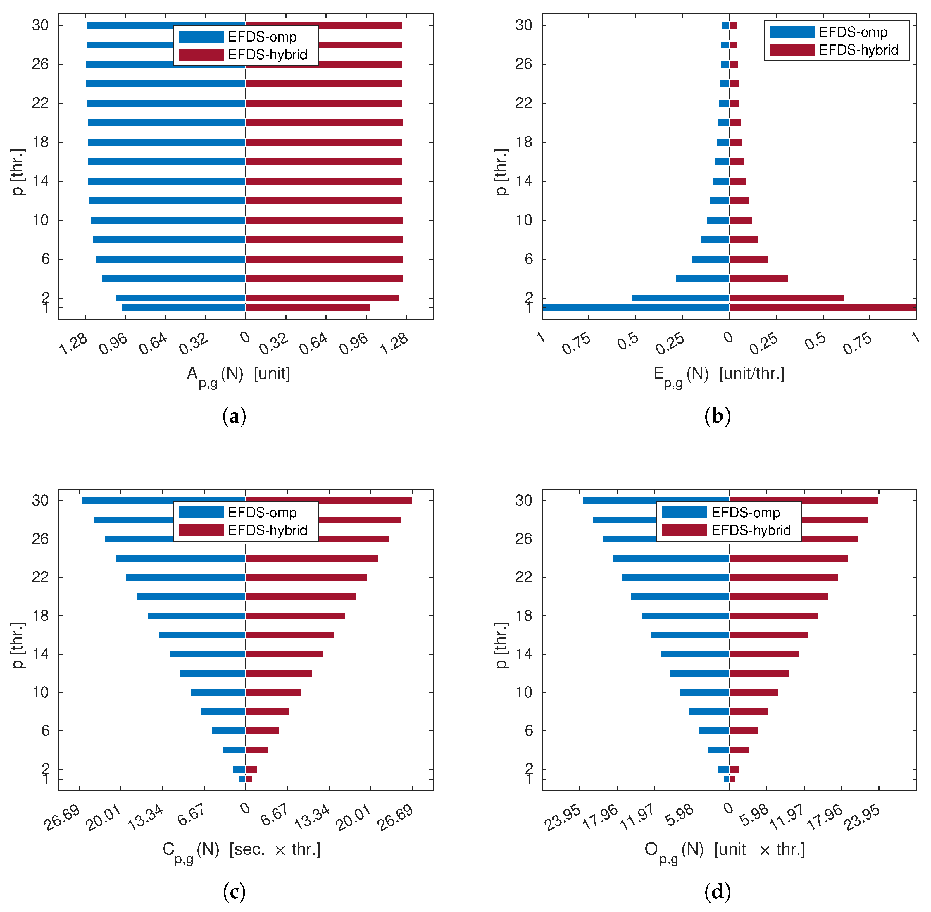
Figure 12 shows the results of analyzing the efficiency of parallel EFDS-omp and EFDS-hybrid algorithms in comparison with their sequential EFDS analog. The results are visualized in the form of demographic diagrams for greater clarity and convenience of displaying two histograms at once on a single figure. From (Figure 12c,d) it can be seen that the cost of parallel algorithms increases linearly and proportionally to the increase in the number of CPU streams involved in the calculations. This may already implicitly indicate the linear nature of the algorithm’s complexity, even before its asymptotic analysis. From (Figure 12a), it can be seen that the EFDS-omp algorithm does not provide any performance gain at all when the number of CPU threads p > 16 increases. In the case of EFDS-hybrid, this occurs even earlier since a significant part of the EFDS-hybrid algorithm is executed either on the GPU or sequentially via a single CPU thread. From (Figure 12b), it can be seen that the efficiency of parallel algorithms does not change significantly when the number of CPU threads, p > 16 , increases, which also indicates that it is not advisable to use p > 16 for calculations.
(Figure 13) shows histograms visualizing the results of analyzing the efficiency of parallel IFDS-MNM-omp and IFDS-MNM-hybrid algorithms in comparison with their sequential IFDS-MNM analog. In all (Figure 13), an increase in the number of CPU threads p > 16 shows a rapid spike in the analyzed performance parameters. This is probably due to the architecture of the CPU used, in particular, the automatic voltage control mechanisms that regulate the CPU clock frequency to protect against overheating. However, from (Figure 13a), it can be seen that the trend towards faster calculations continues when the number of CPU threads increases to p > 16 . This is because the computationally complex operation of calculating the inverse matrix is performed in a parallel OpenMP code block on the CPU in both the IFDS-MNM-omp and IFDS-MNM-hybrid algorithms. From (Figure 12b), it can be seen that the efficiency of parallel algorithms decreases nonlinearly and inversely proportional to the acceleration of calculations depending on p, the number of CPU threads. From (Figure 12c,d), it can be seen that the cost of parallel analogs of IFDS-MNM algorithms increases linearly and is proportional to the number of CPU threads involved, but the rate of increase in cost is much slower than for the EFDS-omp and EFDS-hybrid algorithms (Figure 12c,d). This is because the IFDS-MNM-omp and IFDS-MNM-hybrid algorithms have almost no sequential code blocks and are mostly executed in parallel OpenMP and CUDA code blocks on the CPU and GPU.

8. Complexity Estimates for Parallel Algorithms

From (Figure 11) and the efficiency analysis in (Figure 12 and Figure 13), it can be seen that increasing the number of CPU threads p > 16 will not result in a significant increase in performance. Having thus determined the optimal number of CPU threads to use, similarly to (Table 1), we repeat a series of computational experiments on the four parallel algorithms presented -omp and |-hybrid|at p = 16 , but with the input data size, N, increased by a factor of 5 with a step of 1000 nodes and present the results in (Table 5). Next, using the method from Section 5, based on the data from (Table 5), we will give estimates of the complexity of parallel -omp and -hybrid algorithms.
Indeed, for the parallel algorithms EFDS-omp and EFDS-hybrid (Figure 14a,b), the inequalities (10) hold under the following conditions:
Θ ( n ) = T p , g E F D S - o m p ( N ) = Q n 79.93014 , Q = 0.16784 , k 1 = 0 , k 2 > Q , N 476 ,
Θ ( n ) = T p , g E F D S - h y b r i d ( N ) = Q n 12.51764 , Q = 0.16028 , k 1 = 0 , k 2 > Q , N 78 ,
For the parallel algorithms IFDS-MNM-omp and IFDS-MNM-hybrid (Figure 14c,d), the inequalities (10) hold under the following conditions:
Θ ( n 2 ) = T p , g I F D S - M N M - o m p ( N ) = Q n 2 0.024756 n + 30.07567 , Q = 0.0000034 , k 1 = 0 , k 2 > Q , N 5719 ,
Θ ( n 2 ) = T p , g I F D S - M N M - h y b r i d ( N ) = Q n 2 0.019629 n + 23.692790 , Q = 0.0000027 , k 1 = 0 , k 2 > Q , N 5597 .
where Q is the coefficient for the highest degree of the polynomial, which means that the execution time function of the sequential algorithm T p , g ( N ) is asymptotically bounded from below and above by the polynomial function f p , g ( N ) with an accuracy of a constant k 2 . In other words,
  • For the parallel EFDS-omp and EFDS-hybrid algorithms, the asymptotically exact estimate of time complexity is of the order of Θ ( n ) ;
  • For the parallel IFDS-MNM-omp and IFDS-MNM-hybrid algorithms, the asymptotically exact estimate of time complexity is close to the order of Θ ( n 2 ) .
For the parallel algorithms EFDS-omp and EFDS-hybrid (Figure 15a,c,e), in terms of memory complexity estimates, the relations (10) hold under the following conditions:
Θ ( n 2 ) = M p , g E F D S - o m p ( N ) = Q n 2 + 3.051755 n 0.00416 , Q = 0.190734 , k 1 = 0 , k 2 > 3.24 Q , N 1 ,
Θ ( n 2 ) = M p , g C , E F D S - h y b r i d ( N ) = Q n 2 + 3.051763 n 0.000245 , Q = 0.381469 , k 1 = 0 , k 2 > 3.44 Q , N 1 ,
Θ ( n 2 ) = M p , g G , E F D S - h y b r i d ( N ) = Q n 2 + 2.288813 n 0.003431 , Q = 0.381469 , k 1 = 0 , k 2 > 2.67 Q , N 1 .
Figure 15. Memory usage (Table 6), as well as M functions that interpolate data: (a,c,e) EFDS; (b,d,f) IFDS-MNM.
Computation 13 00252 g015
For the parallel algorithms IFDS-MNM-omp and IFDS-MNM-hybrid (Figure 15b,d,f), in terms of memory complexity estimates, the relations (10) hold under the following conditions:
Θ ( n 2 ) = M p , g I F D S - M N M - o m p ( N ) = Q n 2 + 7.629407 n 0.02745 , Q = 0.762939 , k 1 = 0 , k 2 > 8.41 Q , N 1 ,
Θ ( n 2 ) = M p , g C , I F D S - M N M - h y b r i d ( N ) = Q n 2 + 8.010967 n 0.27193 , Q = 1.525878 , k 1 = 0 , k 2 > 9.26 Q , N 1 ,
Θ ( n 2 ) = M p , g G , I F D S - M N M - h y b r i d ( N ) = Q n 2 + 6.863808 n + 4.1022058 , Q = 1.525879 , k 1 = 0 , k 2 > 12.49 Q , N 1 .
As a result, we have the following:
  • For the parallel EFDS-omp and EFDS-hybrid algorithms, the asymptotically exact estimate of memory complexity is of the order of Θ ( n 2 ) ;
  • For the parallel IFDS-MNM-omp and IFDS-MNM-hybrid algorithms, the asymptotically exact estimate of memory complexity is close to the order of Θ ( n 2 ) .

9. Application of the Discussed Algorithms in Solving Inverse Problems of RVA Dynamics

In this additional section, we will show how the use of the proposed parallel algorithms can accelerate the solution of inverse problems. Let us consider the problem of the mathematical modeling of the dynamics of anomalous variations RVA (1)–(3), but now from the point of view of an inverse problem with the aim of identifying (restoring) the form of the function α ( t ) . In this article, we will skip the theory and details related to the method of solving the inverse problem for equations with fractional derivatives of variable order. They can be found in the works [25,30]. We will only note the following.
First, let the values of the function α ( t ) A C ( 0 , 1 ) (or its mesh analog α ( t i ) A ^ ) be unknown. However, additional information (experimental data) is known about the solution of the difference linear Cauchy problem (1) in the domain Ω ^ :
A ¯ ( t ) = θ ¯ ( t ) , A ¯ ( t i ) = θ ¯ ( t i ) , A ¯ i = θ ¯ i .
Second, let α ( t ) A C ( 0 , 1 ) be a function of a known class, and its form is uniquely determined by a certain set of parameters. Then, the solution to the inverse problem reduces to finding the values of these parameters. Following this approach, we define the set of vectors, X , as the solution space of the inverse problem. Then, the vector X = X 0 , , X K 1 is a set of unknown parameters characterizing the form of the function α ( t ) , where X X , X R K , and K is the number of components.
Third, let us have an idea of the nature of the function α ( t ) = α ( t , X ) A :
α ( t , X ) = 0.99 1 X 0 ( T t ) T cos X 1 t 2 ,
Then, the inverse problem for (1)–(3) is defined as the identification (reconstruction, determination) of the parameters X of the function (24) based on known processing experimental data (23):
0 , t α t , X A ¯ ( t ) = a ( t ) A ¯ ( t ) 2 b ( t ) A ¯ ( t ) + c ( t ) , A ¯ ( t ) = A ( t ) A m a x , A ¯ ( t 0 ) = A 0 A m a x , A ¯ ( t ) = θ ¯ ( t ) , A ¯ ( t 0 ) = θ ¯ ( t 0 ) .
and, in terms of unconditional optimization theory, it is reduced to a minimization problem to be solved via the algorithm [30] based on the iterative Levenberg–Marquardt method [31]. To solve the direct problems that arise, all the EFDS and IFDS-MNM algorithms described above are used in a uniform mesh domain, Ω ^ .
The results of solving the inverse problem (25) are presented (Figure 16), and the time for solving the inverse problem using various algorithms for solving direct problems is presented in (Table 7). As can be seen from the results, the use of the presented parallel algorithms (Figure 7, Figure 8, Figure 9 and Figure 10) can significantly increase the performance of the forward and inverse problem solving tools in the FEVO v1.0 software package, but it is important to use the most appropriate method for solving the forward problem and the algorithm for its implementation. The main selection criterion is the size of the input data N. The use of parallel algorithms can help in cases where, within a single experiment, the inverse problem is solved several times in the process of selecting satisfactory control parameters for the iterative algorithm for solving the inverse problem.
However, it should be noted that the size of the input data, N 10 2 , in a real-world experiment may be smaller than the test data, N 10 4 , used to analyze algorithms for direct problems. In this case, the acceleration of calculations for the inverse problem, one of a series of such problems, will not be as great as that shown in the comparison of algorithms for direct problems (Figure 11). Or, conversely, the use of an inappropriate algorithm will slow down the process of solving the inverse problem, as can be seen from (Table 7).

10. Conclusions

The article has considered various programming implementations of numerical methods for solving the hereditary model equation of radon volumetric activity based on a nonlinear fractional differential equation with a Gerasimov–Caputo derivative of a variable order and variable coefficients. As a result, based on the analysis of the efficiency and complexity estimates of the presented algorithms on a test example, the following results were obtained:
  • The EFDS sequential algorithm has asymptotically exact complexity estimates in both T (time) and RAM (memory) of the order of Θ ( n ) ;
  • The IFDS-MNM sequential algorithm has asymptotically exact complexity estimates in both T (time) and RAM (memory) of the order of Θ ( n 2 ) ;
  • The analysis efficiency and optimal CPU utilization showed that, for all the parallel algorithms considered, increasing the number of CPU threads beyond 16 does not provide a significant performance gain;
  • It has been shown that the parallel algorithms EFDS-omp and -hybrid do not provide a significant increase in calculation speed (approximately 30 % ) compared to EFDS;
  • At the same time, the parallel algorithms IFDS-MNM-omp and IFDS-MNM-hybrid provide a significant increase in computation speed by factors of 13 and 17, respectively, with RAM usage increasing by no more than 2.5 and 5 times, respectively, compared to the sequential IFDS-MNM;
  • The parallel algorithms EFDS-omp and EFDS-hybrid have an asymptotically exact time complexity estimate of order Θ ( n ) , but according to the RAM model, the estimate is of order Θ ( n 2 ) ;
  • The parallel algorithms IFDS-MNM-omp and IFDS-MNM-hybrid have asymptotically exact complexity estimates in terms of T and RAM of order Θ ( n 2 ) ;
  • It can also be seen that, when solving a test example with a uniformly increasing input data size of N and an optimal number of CPU threads of 16, using -hybrid algorithms provides a significant advantage over -omp algorithms only when solving problems with N 15,000, but with the total memory consumption of computing nodes, it is 4 times more. This is due to the fact that operations on vectors and matrices are carried out mainly on the GPU, which offers an advantage over the CPU when working with tensors of large dimensions;
  • The application of the present parallel algorithms can accelerate calculations when solving inverse problems and when selecting an algorithm suitable for the problem.
Based on the results concerning the complexity, efficiency, and optimal usage assessments, several future directions for work can be identified, such as the following: the optimization of the presented parallel algorithms for solving direct problems and the organization of the optimal usage of computer nodes when solving inverse problems via several processes for solving direct problems using hybrid algorithms.

Funding

This work was supported by IKIR FEB RAS State Task (Reg. No. NIOKTR 124012300245-2).

Data Availability Statement

The data presented in this study are available on request from the corresponding author.

Acknowledgments

The author would like to express his special gratitude to his scientific mentor, Parovik Roman, leading researcher at the Institute of Cosmic Radiation Physics, Far Eastern Branch of the RAS, Paratunka, Kamchatka Region, Russia, for his assistance, guidance, and valuable advice. The author would like to express his gratitude to Makarov Evgeny, senior researcher at the Acoustic and Radon Monitoring Laboratory of the Kamchatka Branch of the Unified Geophysical Service of the RAS, Petropavlovsk–Kamchatsky, Russia, for his valuable advice on earthquake precursors and radon monitoring, as well as for providing experimental data from radon-monitoring network stations in the series of works preceding this article devoted to modeling the volumetric activity of radon.

Conflicts of Interest

The author declares no conflicts of interest.

Abbreviations

The following abbreviations are used in this manuscript:
RVARadon Volumetric Actuvity
CPUCentral Processing Unit
GPUGraphic Processing Unit
EFDSExplicit Finite-Difference Scheme
IFDSImplicit Finite-Difference Scheme
MNMModified Newton’s Nethod
OpenMPOpen Multi-Processing
CUDACompute Unified Device Architecture
APIApplication Programming Interface
PRAMParallel Random Access Machine
RAMRandom Access Memory

References

  1. Yasuoka, Y.; Shinogi, M. Anomaly in atmospheric radon concentration: A possible precursor of the 1995 Kobe Japan, earthquake. Health Phys. 1997, 72, 759–761. [Google Scholar] [CrossRef]
  2. Barberio, M.D.; Gori, F.; Barbieri, M.; Billi, A.; Devoti, R.; Doglioni, C.; Petitta, M.; Riguzzi, F.; Rusi, S. Diurnal and Semidiurnal Cyclicity of Radon (222Rn) in Groundwater, Giardino Spring, Central Apennines, Italy. Water 2018, 10, 1276. [Google Scholar] [CrossRef]
  3. Nikolopoulos, D.; Cantzos, D.; Alam, A.; Dimopoulos, S.; Petraki, E. Electromagnetic and Radon Earthquake Precursors. Geosciences 2024, 14, 271. [Google Scholar] [CrossRef]
  4. Petraki, E.; Nikolopoulos, D.; Panagiotaras, D.; Cantzos, D.; Yannakopoulos, P.; Nomicos, C.; Stonham, J. Radon-222: A Potential Short-Term Earthquake Precursor. Earth Sci. Clim. Change 2015, 6, 1000282. [Google Scholar] [CrossRef]
  5. Firstov, P.P.; Makarov, E.O. Dynamics of Subsoil Radon in Kamchatka and Strong Earthquakes; Vitus Bering Kamchatka State University: Petropavlovsk-Kamchatsky, Russia, 2018; p. 148. (In Russian) [Google Scholar]
  6. Dubinchuk, V.T. Radon as a precursor of earthquakes. In Proceedings of the Isotopic Geochemical Precursors of Earthquakes and Volcanic Eruption, Vienna, Austria, 9–12 September 1991; IAEA: Vienna, Austria, 1993; pp. 9–22. [Google Scholar]
  7. Huang, P.; Lv, W.; Huang, R.; Luo, Q.; Yang, Y. Earthquake precursors: A review of key factors influencing radon concentration. J. Environ. Radioact. 2024, 271, 107310. [Google Scholar] [CrossRef]
  8. Kristiansson, K.; Malmqvist, L. Evidence for nondiffusive transport of 86Rn in the ground and a new physical model for the transport. Geophysics 1982, 47, 1444–1452. [Google Scholar] [CrossRef]
  9. Mandelbrot, B.B. The Fractal Geometry of Nature; Times Books: New York, NY, USA, 1982; p. 468. [Google Scholar]
  10. Evangelista, L.R.; Lenzi, E.K. Fractional Anomalous Diffusion. In An Introduction to Anomalous Diffusion and Relaxation; Springer: Berlin/Heidelberg, Germany, 2023; pp. 189–236. [Google Scholar] [CrossRef]
  11. Tverdyi, D.A.; Makarov, E.O.; Parovik, R.I. Hereditary Mathematical Model of the Dynamics of Radon Accumulation in the Accumulation Chamber. Mathematics 2023, 11, 850. [Google Scholar] [CrossRef]
  12. Tverdyi, D.A.; Makarov, E.O.; Parovik, R.I. Research of Stress-Strain State of Geo-Environment by Emanation Methods on the Example of alpha(t)-Model of Radon Transport. Bull. KRASEC Phys. Math. Sci. 2023, 44, 86–104. [Google Scholar] [CrossRef]
  13. Uchaikin, V.V. Fractional Derivatives for Physicists and Engineers. Vol. I. Background and Theory; Springer: Berlin/Heidelberg, Germany, 2013; p. 373. [Google Scholar] [CrossRef]
  14. Parovik, R.I.; Shevtsov, B.M. Radon transfer processes in fractional structure medium. Math. Model. Comput. Simul. 2010, 2, 180–185. [Google Scholar] [CrossRef]
  15. Kilbas, A.A.; Srivastava, H.M.; Trujillo, J.J. Theory and Applications of Fractional Differential Equations, 1st ed.; Elsevier Science: Boston, MA, USA, 2006; p. 540. [Google Scholar]
  16. Cai, M.; Li, C. Theory and Numerical Approximations of Fractional Integrals and Derivatives; Society for Industrial and Applied Mathematics: Philadelphia, PA, USA, 2020; p. 317. [Google Scholar] [CrossRef]
  17. Nakhushev, A.M. Fractional Calculus and Its Application; Fizmatlit: Moscow, Russia, 2003; p. 272. (In Russian) [Google Scholar]
  18. Petras, I. Fractional-Order Nonlinear Systems: Modeling, Analysis and Simulation; Springer: Berlin/Heidelberg, Germany, 2011; p. 218. [Google Scholar]
  19. Patnaik, S.; Hollkamp, J.P.; Semperlotti, F. Applications of variable-order fractional operators: A review. Proc. R. Soc. A 2020, 476, 20190498. [Google Scholar] [CrossRef] [PubMed]
  20. Caputo, M.; Fabrizio, M. On the notion of fractional derivative and applications to the hysteresis phenomena. Meccanica 2017, 52, 3043–3052. [Google Scholar] [CrossRef]
  21. Novozhenova, O.G. Life And Science of Alexey Gerasimov, One of the Pioneers of Fractional Calculus in Soviet Union. FCAA 2017, 20, 790–809. [Google Scholar] [CrossRef]
  22. Shao, J. Mathematical Statistics, 2nd ed.; Springer: New York, NY, USA, 2003; p. 592. [Google Scholar]
  23. Tarantola, A. Inverse Problem Theory: Methods for Data Fitting and Model Parameter Estimation; Elsevier Science Pub. Co.: Amsterdam, The Netherlands; New York, NY, USA, 1987; p. 613. [Google Scholar]
  24. Tverdyi, D.A. Restoration of the order of fractional derivative in the problem of mathematical modelling of radon accumulation in the excess volume of the storage chamber based on the data of Petropavlovsk-Kamchatsky geodynamic polygon. NEWS Kabard.-Balkar. Sci. Cent. RAS 2023, 116, 83–94. [Google Scholar] [CrossRef]
  25. Tverdyi, D.A.; Parovik, R.I.; Makarov, E.O. Estimation of radon flux density changes in temporal vicinity of the Shipunskoe earthquake with MW = 7.0, 17 August 2024 with the use of the hereditary mathematical model. Geosciences 2025, 15, 30. [Google Scholar] [CrossRef]
  26. Mueller, J.L.; Siltanen, S. Linear and Nonlinear Inverse Problems with Practical Applications; Society for Industrial and Applied Mathematics: Philadelphia, PA, USA, 2012; p. 351. [Google Scholar] [CrossRef]
  27. Dennis, J.E., Jr.; Schnabel, R.B. Numerical Methods for Unconstrained Optimization and Nonlinear Equations; SIAM: Philadelphia, PA, USA, 1996; p. 394. [Google Scholar]
  28. Kabanikhin, S.I.; Iskakov, K.T. Optimization Methods for Solving Coefficient Inverse Problems; NGU: Novosibirsk, Russia, 2001; p. 315. (In Russian) [Google Scholar]
  29. Tverdyi, D.A.; Parovik, R.I. The optimization problem for determining the functional dependence of the variable order of the fractional derivative of the Gerasimov-Caputo type. Bull. KRASEC Phys. Math. Sci. 2024, 47, 35–57. (In Russian) [Google Scholar] [CrossRef]
  30. Tverdyi, D.A. Refinement of Variable Order Fractional Derivative of Gerasimov-Caputo Type by Multidimensional Levenberg-Marquardt Optimization Method. In Computing Technologies and Applied Mathematics; Gibadullin, A., Gordin, S., Eds.; CTAM 2024, Springer Proceedings in Mathematics & Statistics; Springer: Berlin/Heidelberg, Germany, 2025; Volume 500, pp. 159–173. [Google Scholar] [CrossRef]
  31. More, J.J. The Levenberg-Marquardt algorithm: Implementation and theory. In Numerical Analysis. Lecture Notes in Mathematics; Watson, G.A., Ed.; Springer: Berlin/Heidelberg, Germany, 1978; Volume 630, pp. 105–116. [Google Scholar] [CrossRef]
  32. Tverdyi, D.A.; Parovik, R.I. Hybrid GPU–CPU Efficient Implementation of a Parallel Numerical Algorithm for Solving the Cauchy Problem for a Nonlinear Differential Riccati Equation of Fractional Variable Order. Mathematics 2023, 11, 3358. [Google Scholar] [CrossRef]
  33. Tverdyi, D.A.; Parovik, R.I. Investigation of Finite-Difference Schemes for the Numerical Solution of a Fractional Nonlinear Equation. Fractal Fract. 2022, 6, 23. [Google Scholar] [CrossRef]
  34. Bogaenko, V.A.; Bulavatskiy, V.M.; Kryvonos, I.G. On Mathematical modeling of Fractional-Differential Dynamics of Flushing Process for Saline Soils with Parallel Algorithms Usage. J. Autom. Inf. Sci. 2016, 48, 1–12. [Google Scholar] [CrossRef]
  35. Bohaienko, V.O. A fast finite-difference algorithm for solving space-fractional filtration equation with a generalised Caputo derivative. Comput. Appl. Math. 2019, 38, 105. [Google Scholar] [CrossRef]
  36. Bohaienko, V.O. Parallel finite-difference algorithms for three-dimensional space-fractional diffusion equation with phi–Caputo derivatives. Comput. Appl. Math. 2020, 39, 163. [Google Scholar] [CrossRef]
  37. Vasilyev, A.V.; Zhukovsky, M.V. Determination of mechanisms and parameters which affect radon entry into a room. J. Environ. Radioact. 2013, 124, 185–190. [Google Scholar] [CrossRef] [PubMed]
  38. Garrappa, R. Numerical Solution of Fractional Differential Equations: A Survey and a Software Tutorial. Mathematics 2018, 6, 16. [Google Scholar] [CrossRef]
  39. Kurnosov, M.G. Introduction to Data Structures and Algorithms: A Textbook; Avtograf: Novosibirsk, Russia, 2015; p. 178. (In Russian) [Google Scholar]
  40. Storer, J.A. An Introduction to Data Structures and Algorithms; Birkhäuser: Boston, MA, USA, 2012; p. 599. [Google Scholar]
  41. Borzunov, S.V.; Kurgalin, S.D.; Flegel, A.V. Workshop on Parallel Programming: A Study Guide; BVH: Saint Petersburg, Russia, 2017; p. 236. (In Russian) [Google Scholar]
  42. Brent, R.P. The parallel evaluation of general arithmetic expressions. J. Assoc. Comput. Mach. 1974, 21, 201–206. [Google Scholar] [CrossRef]
  43. Corman, T.H.; Leiserson, C.E.; Rivet, R.L.; Stein, C. Introduction to Algorithms, 3rd ed.; The MIT Press: Cambridge, UK, 2009; p. 1292. [Google Scholar]
  44. Supinski, B.; Klemm, M. OpenMP Application Programming Interface Specification Version 5.2; Independently Published: North Charleston, SA, USA, 2021; p. 669. [Google Scholar]
  45. Sanders, J.; Kandrot, E. CUDA by Example: An Introduction to General-Purpose GPU Programming; Addison-Wesley Professional: London, UK, 2010; p. 311. [Google Scholar]
  46. Cheng, J.; Grossman, M.; McKercher, T. Professional Cuda C Programming, 1st ed.; Wrox Pr Inc.: New York, NY, USA, 2014; p. 497. [Google Scholar]
  47. King, K.N. C Programming: A Modern Approach, 2nd ed.; W.W. Norton & Company: New York, NY, USA, 2008; p. 832. [Google Scholar]
  48. Kenneth, R. Pointers on C, 1st ed.; Pearson: London, UK, 1997; p. 640. [Google Scholar]
  49. Gergel, V.P.; Strongin, R.G. High Performance Computing for Multi-Core Multiprocessor Systems. Study Guide; Moscow State University Publishing: Moscow, Russia, 2010; p. 544. (In Russian) [Google Scholar]
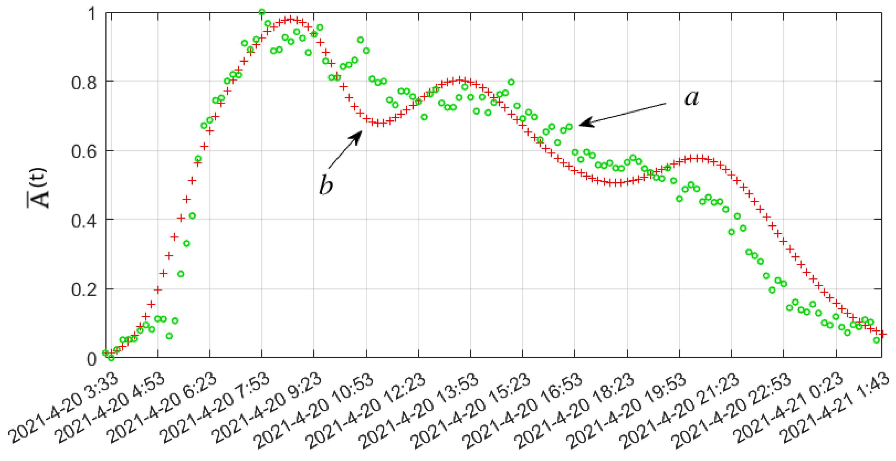
Figure 1. (a) Smoothed and normalized experimental RVA data (isolated anomaly burst) obtained at the MRZR point, with a sampling interval of 1 / 6 [h]; (b) simulation results with a coefficient of determination R 2 = 0.91 and Pearson’s correlation coefficient R = 0.96 .
Computation 13 00252 g001
Figure 2. Results of numerical calculations for the hereditary α ( t ) -model RVA (1) with parameters of the form (2) on a uniform grid (3) at N = 132 : (ac) values of coefficient functions from (2); (d) RVA model curve.
Computation 13 00252 g002
Figure 3. Flowchart of the EFDS sequential algorithm integrated into the FEVO v1.0 software package.
Computation 13 00252 g003
Figure 4. Flowchart of the IFDS-MNM sequential algorithm integrated into the FEVO v1.0.
Computation 13 00252 g004
Figure 5. The execution time of the test example by the algorithms, as well as the function T interpolating the data (Table 1): (a) EFDS; (b) IFDS-MNM.
Computation 13 00252 g005
Figure 7. Flowchart of the EFDS-omp parallel algorithm based on the OpenMP API, integrated into the FEVO v1.0 software package.
Computation 13 00252 g007
Figure 8. Flowchart of the IFDS-MNM-omp parallel algorithm based on the OpenMP API.
Computation 13 00252 g008
Figure 9. Flowchart of the EFDS-hybrid parallel hybrid CPU-GPU algorithm integrated into the FEVO v1.0 software package based on the OpenMP and CUDA API.
Computation 13 00252 g009
Figure 10. Flowchart of the parallel hybrid CPU-GPU algorithm IFDS-MNM-hybrid.
Computation 13 00252 g010
Figure 11. Execution time (Table 3) of the test problem using various parallel algorithms: (a) EFDS; (b) IFDS-MNM.
Computation 13 00252 g011
Figure 12. Efficiency estimation of parallel algorithms EFDS-omp and EFDS-hybrid: (a) acceleration (15); (b) efficiency (16); (c) cost (17); (d) cost-optimal (18).
Computation 13 00252 g012
Figure 13. Efficiency estimation of parallel algorithms IFDS-MNM-omp and IFDS-MNM-hybrid: (a) acceleration (15); (b) efficiency (16); (c) cost (17); (d) cost-optimal (18).
Computation 13 00252 g013
Figure 14. The execution time of the test example using parallel algorithms (Table 5), as well as the function T interpolating the data: (a,b) EFDS; (c,d) IFDS-MNM.
Computation 13 00252 g014
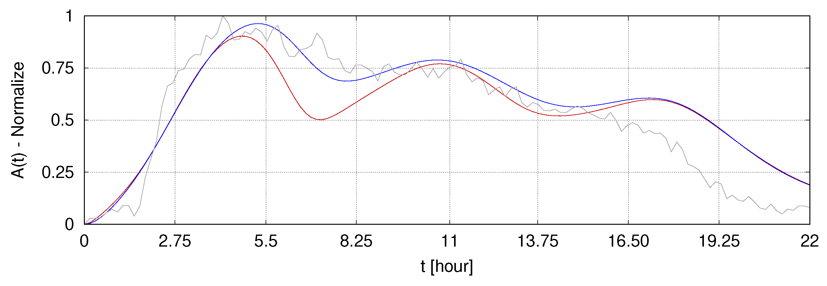
Figure 16. Model curves: (blue)—result of solving the inverse problem (25) based on experimental RVA data; (red)—`benchmark’ solution of the test example (1)–(3) as a direct problem. (Gray)—processed RVA data, similar to (Figure 1).
Computation 13 00252 g016
Table 1. Average execution time for a test example using sequential algorithms.
N20040060080010001200140016001800200022002400260028003000
T 1 , 0 ( N ) , EFDS0.0260.0550.0840.1130.1440.1700.2030.2360.2720.3020.3370.3700.4060.4420.483
T 1 , 0 ( N ) , IFDS-MNM0.0740.2120.4480.8231.3742.0443.0284.4185.8827.8439.99413.1016.6120.9725.75
Table 2. Memory used when solving a test example employing sequential algorithms.
N20040060080010001200140016001800200022002400260028003000
M 1 , 0 ( N ) , EFDS0.0060.0120.0180.0240.0300.0360.0420.0480.0540.0610.0670.0730.0790.0850.091
M 1 , 0 ( N ) , IFDS-MNM0.2430.9442.1033.7205.7948.32611.3114.7618.6623.0327.8533.1338.8645.0651.71
Table 3. Average execution time test example (with N = 6000 ) using various parallel algorithms.
p T p , 0 ( N )
EFDS
-omp
T p , g ( N )
EFDS
-hybrid
T p , 0 ( N )
IFDS-MNM
-omp
T p , g ( N )
IFDS-MNM
-hybrid
21.0680.903147.388115.829
40.9630.88376.35558.927
60.9270.88450.78040.516
80.9060.88439.47930.801
100.8940.88432.37325.315
120.8850.88627.07121.527
140.8790.88723.88718.934
160.8780.88621.32516.810
180.8760.88625.70023.091
200.8800.88523.97721.175
220.8740.88621.96319.667
240.8680.88620.62918.510
260.8690.88719.74717.398
280.8710.88818.53816.427
300.8750.88917.63815.799
Table 4. Memory usage for solving the test example (with N = 6000 ) using different algorithms.
M p , 0 ( N )
EFDS
-omp
M p , g C ( N )
EFDS
-hybrid
M p , g G ( N )
EFDS
-hybrid
M p , 0 ( N )
IFDS-MNM
-omp
M p , g C ( N )
IFDS-MNM
-hybrid
M p , g G ( N )
IFDS-MNM
-hybrid
RAM–
M 1 , 0 ( N ) alg.
0.1830206.4280
RAM68.847137.512137.466275.115549.797549.728
Table 5. The average execution time of the test example using various parallel algorithms with p = 16 .
N T p , 0 ( N )
EFDS
-omp
T p , g ( N )
EFDS
-hybrid
T p , 0 ( N )
IFDS-MNM
-omp
T p , g ( N )
IFDS-MNM
-hybrid
10000.1380.1400.3770.337
20000.2820.2741.0950.985
30000.4200.4142.7352.388
40000.5680.5585.5134.965
50000.7210.72811.45510.288
60000.8780.89220.91816.829
70001.0421.05033.81228.511
80001.2221.22452.33742.891
90001.3921.39474.27063.681
10,0001.5591.569103.68585.078
11,0001.7431.752143.353126.858
12,0001.9391.944193.125159.268
13,0002.1242.145264.476225.509
14,0002.3272.320365.500275.562
15,0002.5072.516465.145391.044
Table 6. Memory usage when solving the test example with various parallel algorithms at p = 16 .
N M p , 0 ( N )
EFDS
-omp
M p , g C ( N )
EFDS
-hybrid
M p , g G ( N )
EFDS
-hybrid
M p , 0 ( N )
IFDS-MNM
-omp
M p , g C ( N )
IFDS-MNM
-hybrid
M p , g G ( N )
IFDS-MNM
-hybrid
10001.9383.8453.8387.70615.33915.327
20007.69015.32015.30530.67061.19561.172
300017.25834.42434.40168.893137.569137.535
400030.64061.15761.127122.375244.461244.415
500047.83695.52095.482191.116381.870381.813
600068.848137.512137.466275.116549.797549.728
700093.674187.134187.080374.374748.241748.161
8000122.314244.385244.324488.892977.203977.112
9000154.770309.265309.196618.6681236.6831236.580
10,000191.040381.775381.699763.7021526.6801526.566
11,000231.125461.914461.830923.9961847.1951847.069
12,000275.024549.683549.5911099.5482198.2272198.090
13,000322.739645.081644.9811290.3592579.7772579.628
14,000374.268748.108748.0011496.4292991.8442991.684
15,000429.611858.765858.6501717.7583434.4293434.258
Table 7. Solution time in [sec] for the inverse problem when using various algorithms to solve direct problems.
Sequential, p = 1 -omp, p = 16 -hybrid, p = 16
EFDS0.0580.10.242
IFDS-MNM1.5150.6620.893
Disclaimer/Publisher’s Note: The statements, opinions and data contained in all publications are solely those of the individual author(s) and contributor(s) and not of MDPI and/or the editor(s). MDPI and/or the editor(s) disclaim responsibility for any injury to people or property resulting from any ideas, methods, instructions or products referred to in the content.