Stock Price Prediction in the Financial Market Using Machine Learning Models

Abstract

This paper presents an analysis of stock price forecasting in the financial market, with an emphasis on approaches based on time series models and deep learning techniques. Fundamental concepts of technical analysis are explored, such as exponential and simple averages, and various global indices are analyzed to be used as inputs for machine learning models, including Recurrent Neural Network (RNN), Long Short-Term Memory (LSTM), Gated Recurrent Unit (GRU), Convolutional Neural Network (CNN), and XGBoost. The results show that while each model possesses distinct characteristics, selecting the most efficient approach heavily depends on the specific data and forecasting objectives. The complexity of advanced models such as XGBoost and GRU is reflected in their overall performance, suggesting that they can be particularly effective at capturing patterns and making accurate predictions in more complex time series, such as stock prices.

1. Introduction

The fusion between technology and finance has radically transformed the way markets operate and how investors make decisions. With the emergence of online trading platforms, high-frequency trading algorithms and the increasing use of Artificial Intelligence (AI), the financial landscape is experiencing an unprecedented digital revolution.

This convergence is redefining the boundaries of what is possible in the stock market, offering new opportunities and challenges for investors and analysts. The ability to process large volumes of data in real time and apply advanced analytics algorithms is creating new opportunities in forecasting and risk management. In this context, the research and development of AI-based forecasting models represents a growing area of interest [1].

The stock market is a global environment where millions of investors buy and sell shares in companies, representing a fraction of a company’s share capital. The purpose of these transactions is to profit from fluctuations in asset prices. For many, investing in the stock market is an essential part of their financial strategy, as it offers an opportunity to grow their capital over time in a passive way, often surpassing the rates of return offered by more traditional investments, such as bank deposits. However, stock market trading is also known for its unpredictability and high volatility. Predicting future market movements is a challenging and highly desirable task. Investors are constantly looking for new methods and techniques to anticipate market changes and make more informed decisions about their investment portfolios.

Throughout history, investors and analysts have employed a variety of methods and techniques to anticipate stock market behavior. From fundamental analysis, which evaluates financial performance and potential company growth, to technical analysis, which examines past price patterns to identify future trends, a wide range of approaches have been explored. However, even with all these efforts, the ability to accurately predict market movements remains a challenging and evolving open issue.

Recently, with technological advances and increasing data availability, new opportunities have emerged to apply machine learning (ML) techniques in stock market forecasts. ML, a subfield of AI, focuses on the development of algorithms capable of learning patterns and making data-driven predictions. By analyzing vast sets of historical data, algorithm ML tools can identify complex correlations and subtle patterns that might otherwise be missed to traditional forecasting methods [2].

In this work, we aim to explore the potential of ML algorithms in stock market prediction. Predictive models are developed to capture the complexity and dynamics of the market, providing valuable insights for investors. By combining advanced ML techniques with an in-depth understanding of financial markets, this study seeks to contribute to the advancement of the field and deliver tangible benefits to those operating in the stock market. For that, this study distinguishes from other works by establishing a basis in the field of time series forecasting in the stock market, not only by choosing between various algorithms, such as LSTM, GRU, CNN, RNN, XGBoost, but also by choosing different combinations of these, for instance, LSTM + CNN, LSTM + GRU, GRU + CNN, RNN + GRU, and RNN + LSTM, and for different numbers of layers for each model and combination of algorithms. More detailed analysis in the selection of the best features, window input size, and hyperparameters is also provided. The main contributions of this work are as follows:

• Providing a basic understanding of how the stock market works and how ML is being used to predict it.
• Evaluating which features are best suited to be used as inputs to stock market prediction models.
• Developing and applying various ML models for stock price prediction.
• Evaluating and comparing the performance of different models using a variety of metrics to identify which techniques and combination of techniques provide the best results in stock price prediction.

The article is structured as follows. Section 2 describes the dataset utilized, the evaluation metrics applied, and the data preparation process for the models. Section 3 introduces the forecasting models employed for stock price prediction. Section 4 presents the results of the study, including a comparative analysis of the applied forecast models. Section 5 provides a discussion of the results. Finally, Section 6 addresses the main conclusions and outlines potential directions for future work.

Literature Review

In recent years, the application of machine learning and deep learning techniques in financial markets has garnered significant interest, particularly for stock market price forecasting. One study by Zhenglin Li et al. (2023) investigated the use of Long Short-Term Memory (LSTM) networks to predict the stock prices of major technology companies, including Apple Inc. (Cupertino, CA, USA); Alphabet Inc. (Mountain View, CA, USA), owner of Google; Microsoft Corporation, Inc. (Redmond, WA, USA) and Amazon.com, Inc. (Seattle, WA, USA and Arlington, VI, USA) [3]. The researchers utilized historical stock price data from Yahoo Finance, spanning over a decade, to train their LSTM model. The study demonstrated that LSTM effectively shared the potential of capturing complex patterns and trends in stock price movements, leading to reasonably accurate predictions. However, the authors highlighted limitations, such as the need for a larger dataset and the use of additional evaluation metrics, in addition to the used RMSE, to provide a more comprehensive performance analysis. Sonkavde et al. (2023) provided a systematic review of machine learning and deep learning techniques in financial forecasting, emphasizing ensemble models such as a hybrid of Random Forest, XGBoost, and LSTM. Their findings concluded that these models outperform individual algorithms, offering improved accuracy and reduced errors in stock price predictions. By implementing and testing ensemble methods on specific stock datasets, the study confirms the potential of integrated approaches to address the complexities of financial data [4]. Hoque and Aljamaan (2021) conducted a detailed study on the impact of hyperparameter tuning on the performance of machine learning models in stock price forecasting. Their research focused on the Saudi Stock Exchange. This study’s goal was to evaluate and compare the predictive capabilities of eight machine learning models, including Decision Trees (DTs), Support Vector Regression (SVR), K-Nearest Neighbors (KNN), Gaussian Process Regression (GPR), Stochastic Gradient Descent (SGD), Partial Least Squares Regression (PLS), Kernel Ridge Regression (KRR), and Least Absolute Shrinkage And Selection Operator (LASSO), both with and without hyperparameter tuning. The study’s conclusions were significant: hyperparameter tuning substantially improved the forecasting accuracy of most models, with SVR emerging as the best performer after tuning. Additionally, the research emphasized that the default hyperparameter configurations of machine learning models are often suboptimal, and tuning is essential for achieving robust predictions. This insight is particularly valuable for practitioners and researchers aiming to apply machine learning techniques in financial markets [5]. Gülmez et al. (2023) introduced a novel approach combining LSTM with the Artificial Rabbits Optimization (ARO) algorithm to enhance the prediction accuracy of stock prices. This study focused on the Dow Jones Industrial Average (DJIA) index and evaluated the model against various alternatives, including traditional Artificial Neural Networks (ANNs), unoptimized LSTMs, and LSTMs optimized using Genetic Algorithms (GAs). To benchmark the performance, the research employed multiple evaluation metrics, such as Mean Squared Error (MSE), Mean Absolute Error (MAE), Mean Absolute Percentage Error (MAPE), and $R^2$. Among these metrics, the LSTM-ARO model exhibited the lowest error rates (MSE, MAE, and MAPE) and the highest $R^2$, indicating its superior ability to model the financial data [6]. Another contribution by Nabipour et al. (2020) explored the effectiveness of various machine learning models, including Decision Tree, Bagging, Random Forest, Adaptive Boosting (Adaboost), Gradient Boosting, and XGBoost, ANNs, recurrent neural network (RNN), and LSTMs, in predicting the stock market groups within the Tehran Stock Exchange. Using a decade of historical data and technical indicators as input features, the study highlighted that LSTM demonstrated superior accuracy compared to other models. The research emphasized the importance of deep learning techniques in managing the inherent non-linearity while also recommending the exploration of ensemble approaches for enhanced performance and the use on different stock markets [7]. Naufal and Wibowo (2023) proposed a hybrid deep learning model integrating Convolutional Neural Network (CNN), LSTM, and Gated Recurrent Units (GRUs) for stock price forecasting across Tesla, Inc., Alphabet Inc., and Twitter, Inc. when it was public. By combining the strengths of these architectures, the hybrid model achieved improved prediction accuracy over standalone LSTM networks, effectively addressing both the short- and long-term dependencies in stock data. The study concluded that hybrid models are particularly advantageous in managing the complexities of the dynamic and non-linear stock market trends [8]. Zhang et al. (2023) proposed an hybrid model combining CNN, BiLSTM, and a mechanism for stock price prediction, addressing the non-linear, volatile, and high-frequency nature of financial data. The model leverages the ability of CNNs to extract local non-linear features, along with the capacity of BiLSTM to capture bidirectional temporal features. Additionally, an attention mechanism was incorporated to fit the weight assignments to the information features automatically, enhancing prediction accuracy. The model was tested on 12 stock indices, including the CSI 300 from China and 8 international markets, consistently demonstrating superior performance compared to alternatives such as the standalone LSTM, CNN-LSTM, and CNN-Attention models in the previous mentioned works. Evaluation metrics such as RMSE, MAPE, and $R^2$ confirmed the model’s accuracy in handling diverse market data [9]. Mehtab and Sen (2020) introduced a suite of five deep learning-based regression models for forecasting the NIFTY 50 index, using historical data from December 2008 to July 2020. The proposed models included two CNN-based architectures and three variants of LSTM models, evaluated using a multi-step prediction approach with walk-forward validation. Among these, the encoder–decoder CNN-LSTM model, which utilized two weeks of historical data, achieved the highest prediction accuracy, while the univariate CNN model with one week of data was the fastest in terms of execution. Their study highlighted the ability of hybrid architectures to effectively capture complex temporal patterns in financial time series, offering both accuracy and computational efficiency. The authors also suggested the potential for future research involving generative adversarial networks (GANs) to improve forecasting accuracy [10].

2. Materials and Methods

In this section, the development of the techniques and processes used are discussed. It begins with a description of the dataset used, followed by the presentation and description of all the features integrated into the dataset. Finally, the methods used to make predictions are detailed through the algorithms and the presentation of the developed models.

2.1. Dataset

The initial dataset is composed of historic data of Apple Inc. collected from Yahoo Finance [11]. This dataset includes over 40 years of stock prices and is organized in 7 columns, containing the Open, High, Low, Close, and Adjusted Close prices, as well as the date and the volume of transactions, as shown in Table 1.

Table 1. Apple dataset.

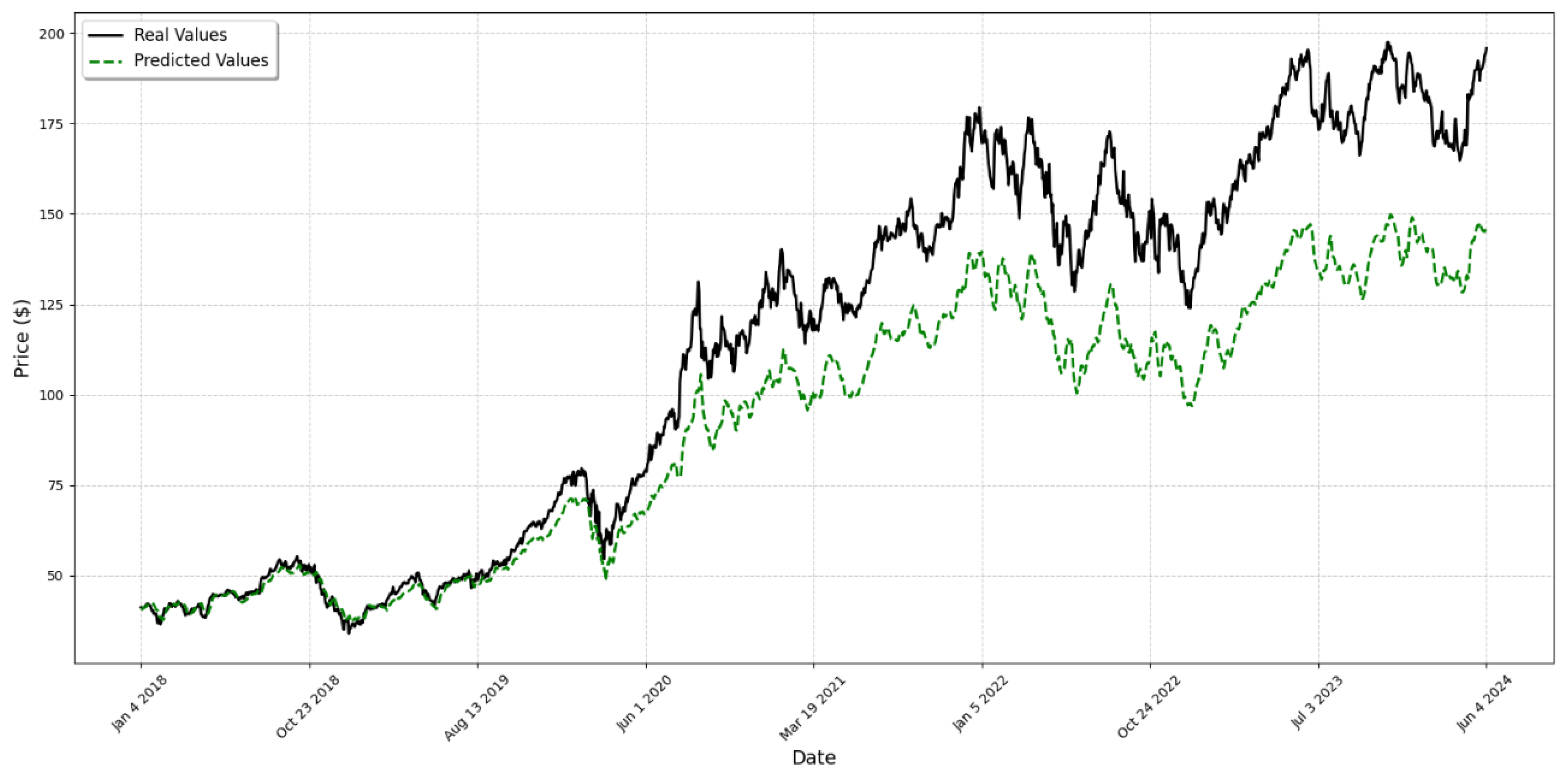
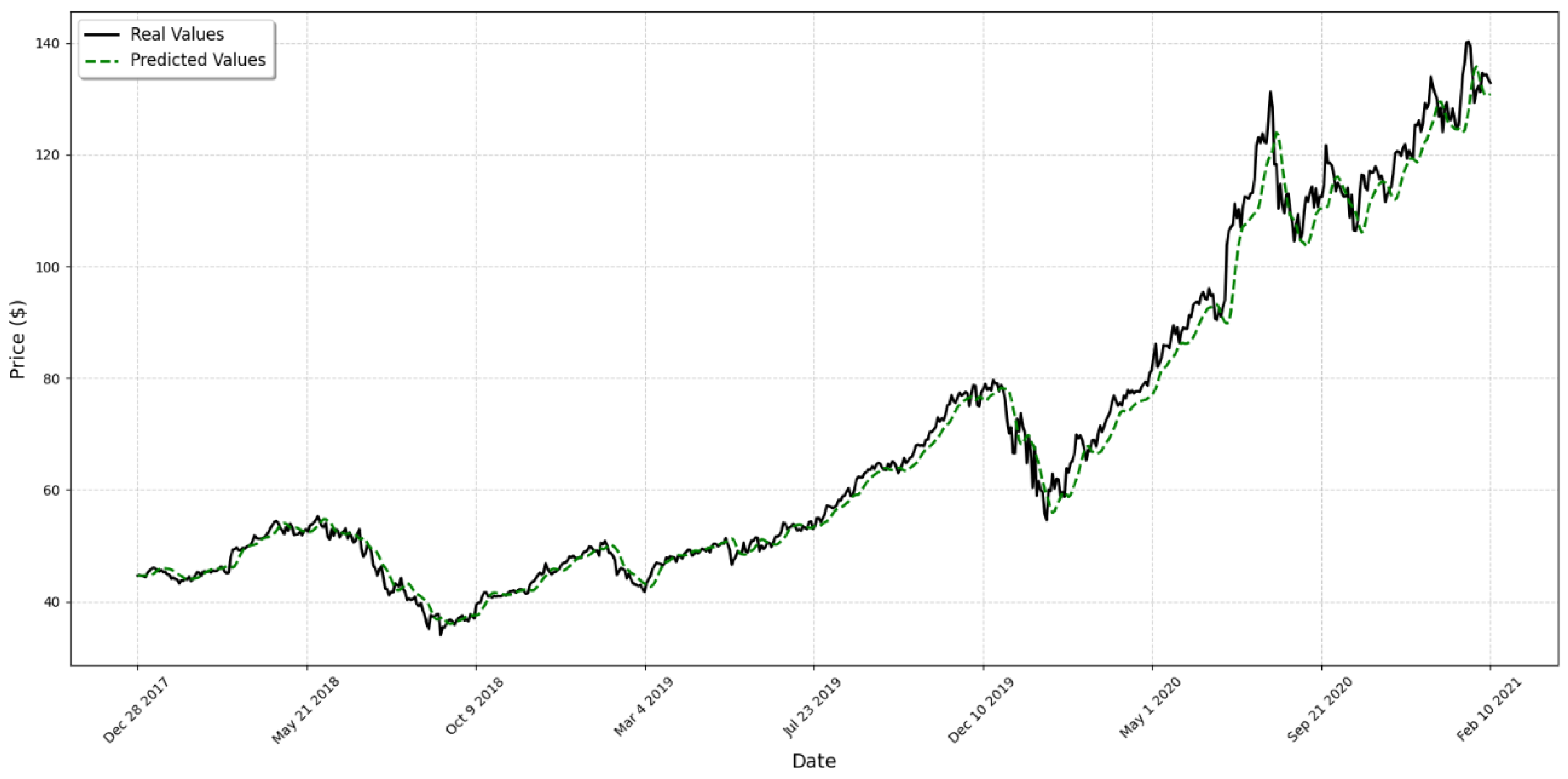
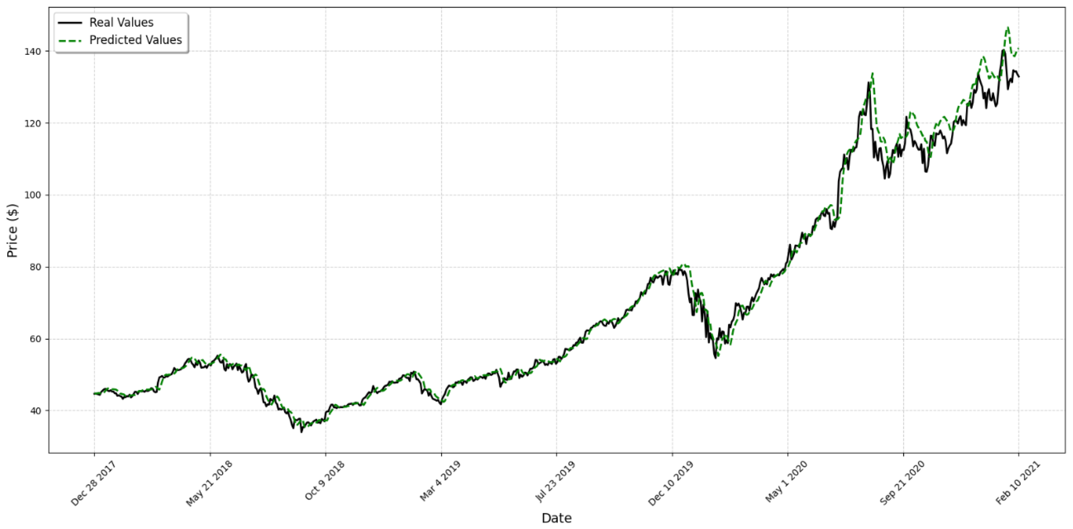
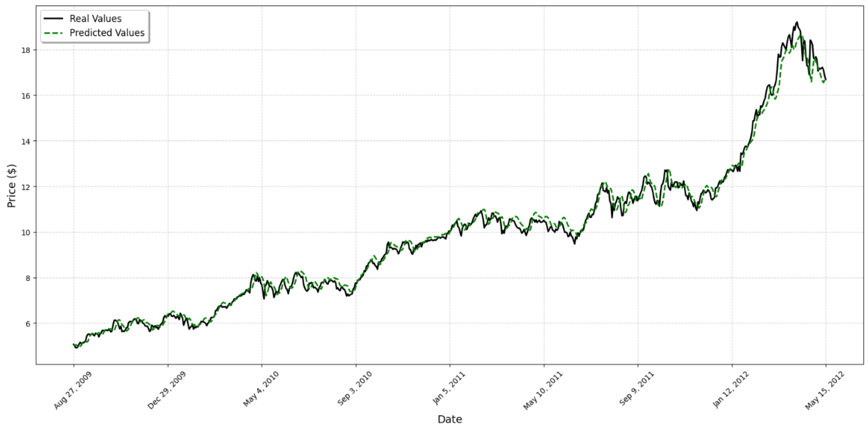
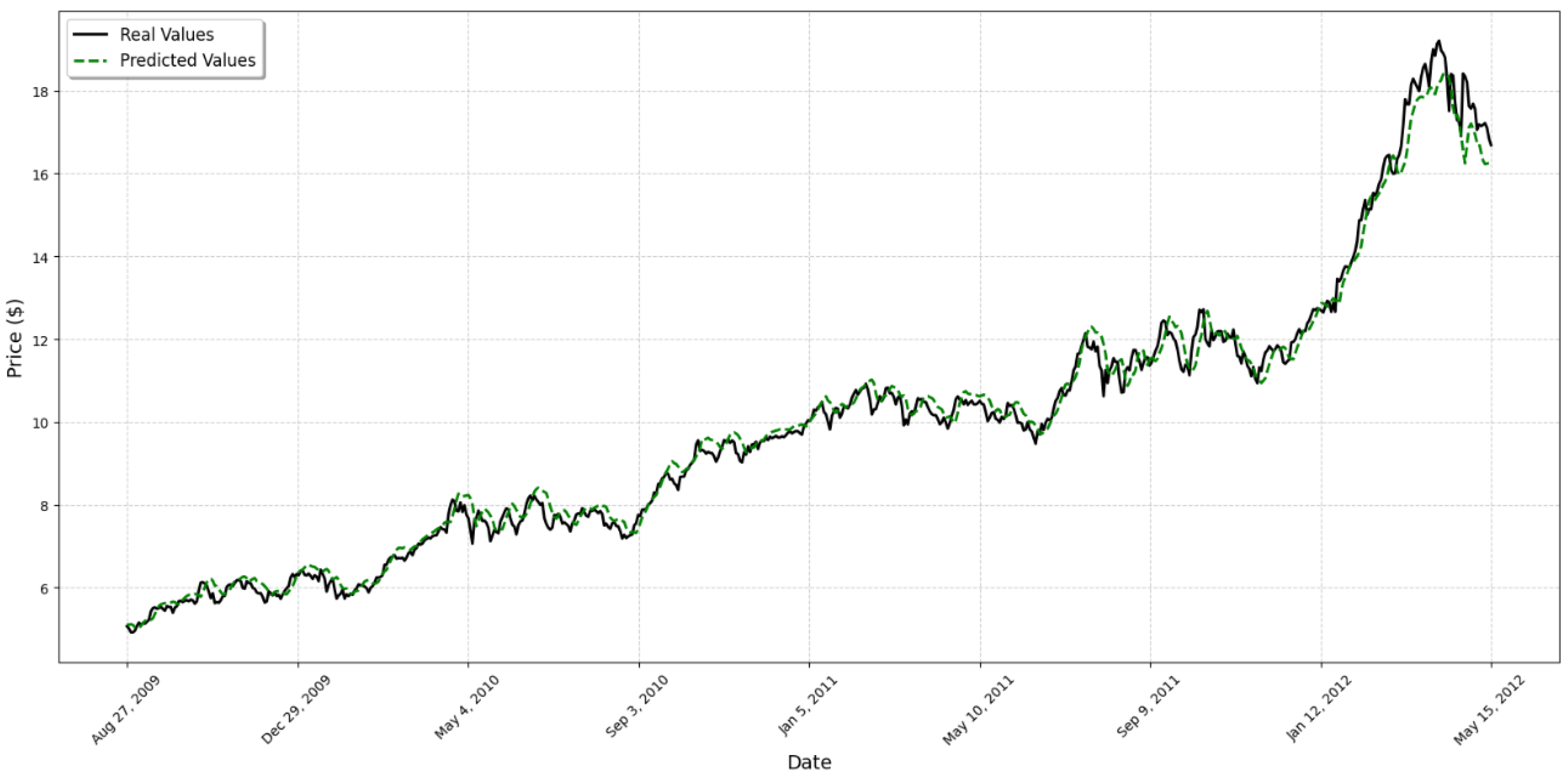
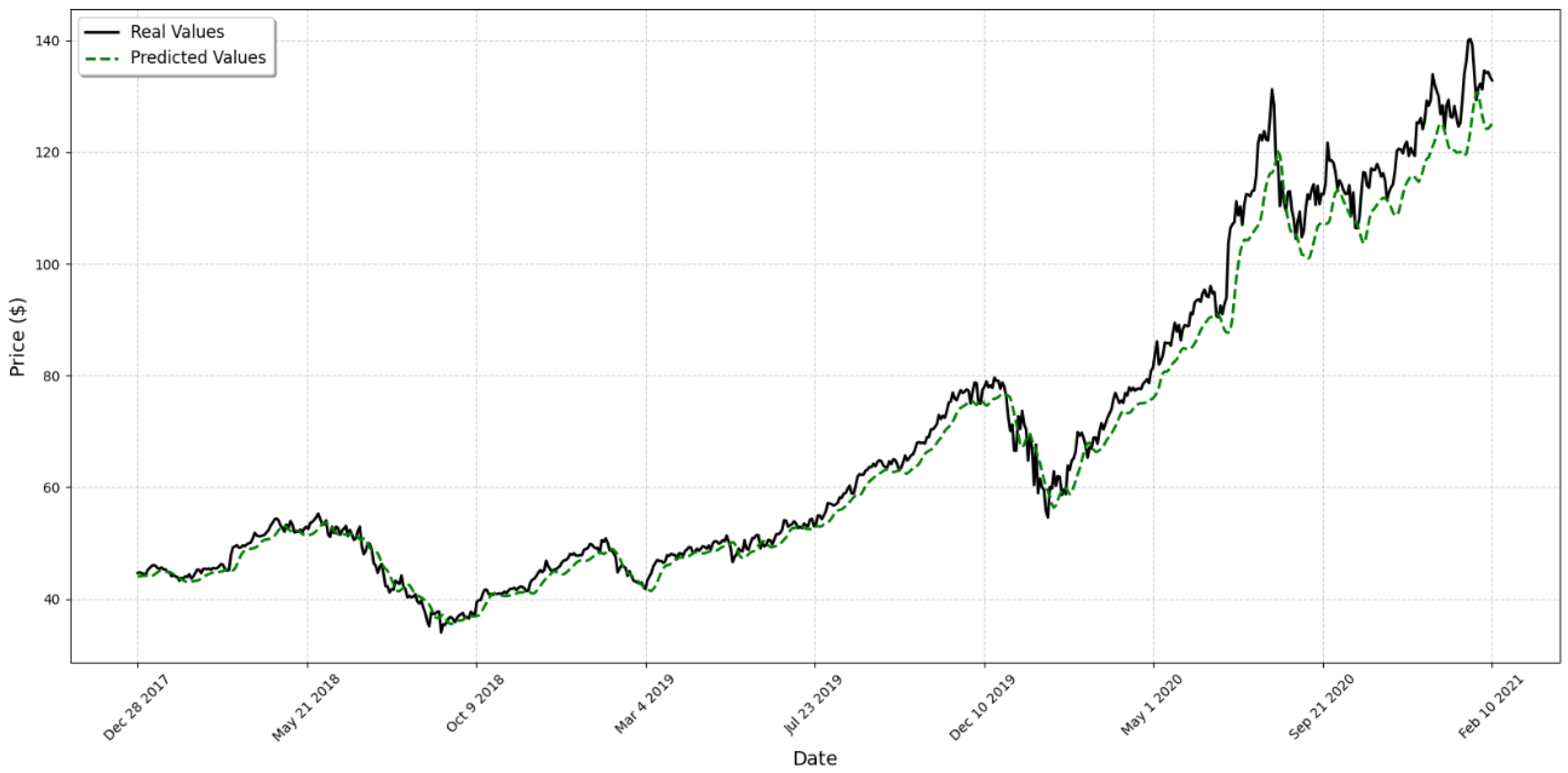
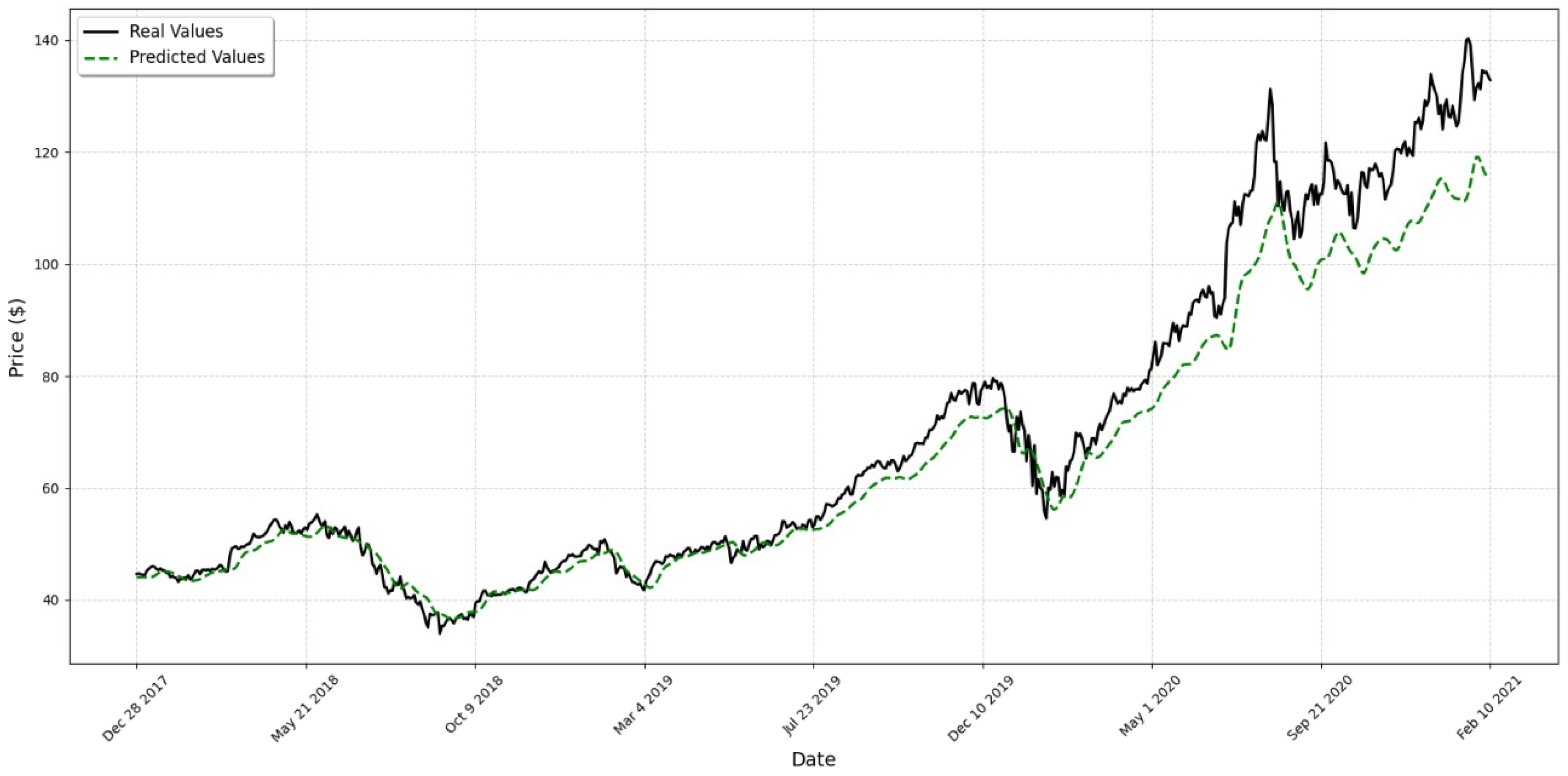
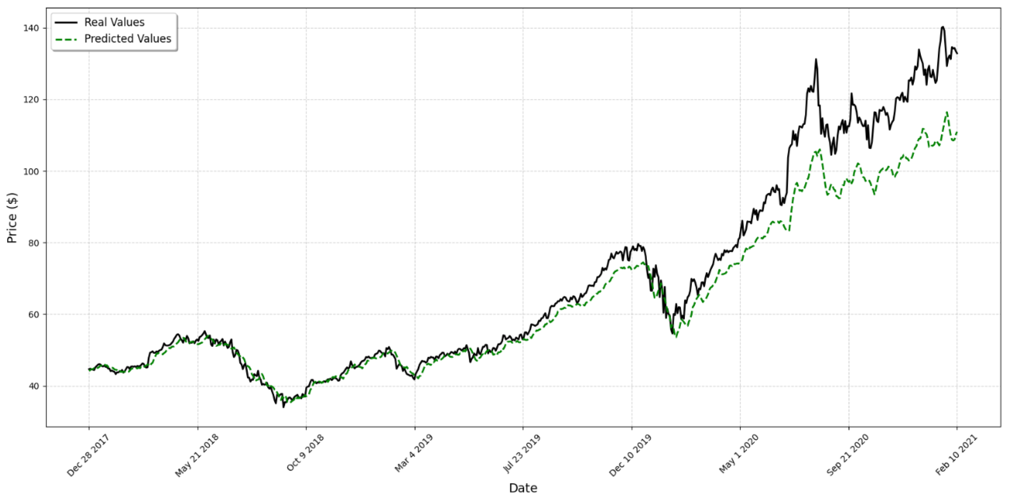
Date	Open	High	Low	Close	Adj Close 1	Volume
1980-12-12	0.128348	0.128906	0.128348	0.128348	0.098943	469,033,600
1980-12-15	0.122210	0.122210	0.121652	0.121652	0.093781	175,884,800
1980-12-16	0.113281	0.113281	0.112723	0.112723	0.086898	105,728,000
1980-12-17	0.115513	0.116071	0.115513	0.115513	0.089049	86,441,600
1980-12-18	0.118862	0.119420	0.118862	0.118862	0.091630	73,449,600

¹ Adjusted Close.

2.2. Features

Another 43 features were also added to the initial dataset and tested using both the correlation method and SelectKBest, based on their relationship with the target variable, set to be the value of the Adj Close price [12,13]. The first 27 features are directly related to Apple Inc. stock, including price data, transaction volume, and technical indicators such as moving averages and momentum metrics. The other features are a combination of interest rates and indices.

All features were selected based on their popularity, including Exponential Moving Averages and Simple Moving Averages, as well as those identified in the study by Hoseinzade, Ehsan and Haratizadeh, Saman [14]. This study evaluates a diverse array of variables for use as features in prediction models. These features were either calculated or gathered using several sources, including Yahoo Finance, the Federal Reserve Economic Data (FRED), which is an online database managed by the Federal Reserve Bank of St. Louis [15], and the Pandas Technical Analysis library, TA-Lib, which offers a comprehensive set of technical indicators [12]. A complete list of these features can be found in Table 2.

Table 2. Features tested.

#	Variable	Description	Type	Source
1	Open	Open Price	Price	Yahoo Finance
2	High	Highest Price	Price	Yahoo Finance
3	Low	Lowest Price	Price	Yahoo Finance
4	Close	Closing Price	Price	Yahoo Finance
5	Adj Close	Adjusted Closing Price	Price	Yahoo Finance
6	Volume	Volume of transactions	Volume	Yahoo Finance
7	MOM2	2-day momentum	Technical Indicator	Calculated
8	MOM3	3-day momentum	Technical Indicator	Calculated
9	MOM4	4-day momentum	Technical Indicator	Calculated
10	MACD	Moving Average Convergence/Divergence		TA-Lib
11	RSI	Relative Strength Index	Technical Indicator	TA-Lib
12	ROC5	5-day Rate of Change	Technical Indicator	TA-Lib
13	ROC10	10-day Rate of Change	Technical Indicator	TA-Lib
14	ROC15	15-day Rate of Change	Technical Indicator	TA-Lib
15	ROC20	20-day Rate of Change	Technical Indicator	TA-Lib
16	SMA5	5-day Simple Moving Average	Technical Indicator	TA-Lib
17	SMA25	25-day Simple Moving Average	Technical Indicator	TA-Lib
18	SMA50	50-day Simple Moving Average	Technical Indicator	TA-Lib
19	SMA100	100-day Simple Moving Average	Technical Indicator	TA-Lib
20	SMA200	200-day Simple Moving Average	Technical Indicator	TA-Lib
21	EMA10	10-day Exponential Moving Average	Technical Indicator	TA-Lib
22	EMA12	12-day Exponential Moving Average	Technical Indicator	TA-Lib
23	EMA20	20-day Exponential Moving Average	Technical Indicator	TA-Lib
24	EMA26	26-day Exponential Moving Average	Technical Indicator	TA-Lib
25	EMA50	50-day Exponential Moving Average	Technical Indicator	TA-Lib
26	EMA100	100-day Exponential Moving Average	Technical Indicator	TA-Lib
27	EMA200	200-day Exponential Moving Average	Technical Indicator	TA-Lib
28	DTB4WK	4-Week Treasury Bill	Interest Rate	FRED
29	DTB3	3-Month Treasury Bill	Interest Rate	FRED
30	DTB6	6-Month Treasury Bill	Interest Rate	FRED
31	DGS5	5-Year Treasury Constant Maturity Rate	Interest Rate	FRED
32	DGS10	10-Year Treasury Constant Maturity Rate	Interest Rate	FRED
33	DAAA	Moody’s Seasoned Aaa Corporate Bond Yield	Interest Rate	FRED
34	DBAA	Moody’s Seasoned Baa Corporate Bond Yield	Interest Rate	FRED
35	TE1	DGS10-DTB4WK	Interest Rate Spread	Calculated
36	TE2	DGS10-DTB3	Interest Rate Spread	Calculated
37	TE3	DGS10-DTB6	Interest Rate Spread	Calculated
38	TE5	DTB3-DTB4WK	Interest Rate Spread	Calculated
39	TE6	DTB6-DTB4WK	Interest Rate Spread	Calculated
40	DE1	DBAA-BAAA	Credit Spread	Calculated
41	DE2	DBAA-DGS10	Technical Indicator	Calculated
42	DE4	DBAA-DTB6	Technical Indicator	Calculated
43	DE5	DBAA-DTB3	Technical Indicator	Calculated
44	DE6	DBAA-DTB4WK	Technical Indicator	Calculated
45	DCOILWTICO	Crude Oil Prices: West Texas Intermediate (WTI)	Commodity	FRED
46	IXIC	NASDAQ Composite Index	Index	Yahoo Finance
47	GSPC	S&P 500 Index	Index	Yahoo Finance
48	DJI	Dow Jones Industrial Index	Index	Yahoo Finance
49	NYA	NYSE Composite Index	Index	Yahoo Finance

Starting with the correlation analysis, the results can be observed in Table 3. This table indicates the correlation of all features with the target variable. Correlation analysis is a fundamental approach for understanding the relationship between all features and the target variable. It is noteworthy that the top 20 features exhibit significantly higher correlation values compared to the others, as these are variables related to the price, moving averages, or indices, which naturally track stock prices fluctuations closely.

Table 3. Correlation.

Nº	Feature	Correlation	Nº	Feature	Correlation
1	Adj Close	0.999757	26	DCOILWTICO	0.163709
2	Low	0.999527	27	TE6	0.140110
3	High	0.999503	28	MOM5	0.089892
4	Open	0.999411	29	MOM4	0.080078
5	SMA5	0.999335	30	MOM3	0.067845
6	EMA10	0.999167	31	MOM2	0.052424
7	EMA12	0.999064	32	RSI	0.007301
8	EMA20	0.998661	33	ROC5	−0.014739
9	EMA26	0.998375	34	ROC10	−0.017959
10	SMA25	0.997924	35	ROC15	−0.021291
11	EMA50	0.997375	36	ROC20	−0.023569
12	SMA50	0.996326	37	DGS5	−0.116094
13	EMA100	0.995705	38	DE1	−0.169746
14	SMA100	0.994129	39	DE2	−0.325379
15	EMA200	0.992936	40	DGS10	−0.327576
16	SMA200	0.990444	41	Volume	−0.472102
17	IXIC	0.963824	42	DBAA	−0.495441
18	GSPC	0.955474	43	DAAA	−0.502339
19	DJI	0.931631	44	DE6	−0.524144
20	NYA	0.876839	45	TE1	−0.533726
21	MACD	0.266051	46	DE5	−0.538855
22	TE5	0.228270	47	DE4	−0.543380
23	DTB3	0.185540	48	TE2	−0.556787
24	DTB6	0.184989	49	TE3	−0.563363
25	DTB4WK	0.166905

In addition to the correlation analysis, the SelectKBest method was employed to select the best features. This method is one of the most commonly used feature selection techniques and is based on machine learning filters. It utilizes statistical tests to identify features that have the strongest relationship with the output variable, with the procedure initially involving the definition of the appropriate statistical test based on the type of data and the problem at hand. In regression cases, the SelectKBest method provides the f_regression option, which was utilized here to select the best features [16]. Subsequently the test was applied to each feature to calculate an importance score. Features with the highest scores were selected, and the dataset was transformed to include only these features. Upon applying this method to the 49 features, scores for each were obtained as evidenced in Table 4.

Table 4. SelectKBest score.

Nº	Feature	Score	Nº	Feature	Score
1	Adj Close	11,500,000	26	DE6	2120
2	Low	5,900,000	27	DAAA	1890
3	High	5,630,000	28	DBAA	1820
4	Open	4,740,000	29	Volume	1600
5	SMA5	4,200,000	30	DGS10	672
6	EMA10	3,350,000	31	DE2	662
7	EMA12	2,980,000	32	MACD	6.72
8	EMA20	2,080,000	33	TE5	307
9	EMA26	1,720,000	34	DTB3	199
10	SMA25	1,340,000	35	DTB6	198
11	EMA50	1,060,000	36	DE1	166
12	SMA50	756,000	37	DTB4WK	160
13	EMA100	647,000	38	DCOILWTICO	154
14	SMA100	472,000	39	TE6	112
15	EMA200	392,000	40	DGS5	76.4
16	SMA200	288,000	41	MOM5	45.6
17	IXIC	73,100	42	MOM4	36.1
18	GSPC	58,600	43	MOM3	25.9
19	DJI	36,800	44	MOM2	15.4
20	NYA	18,600	45	ROC20	3.11
21	TE3	2600	46	ROC15	2.54
22	TE2	2510	47	ROC10	1.80
23	DE4	2340	48	ROC5	1.22
24	DE5	2290	49	RSI	0.298
25	TE1	2230

Analyzing Table 3 and Table 4, it can be concluded that the performance of the top 20 features does not vary between the two selection methods. Furthermore, the top 20 features achieved much higher scores than the others, particularly in the correlation analysis, where the 20th best feature (NYA) scored $0.876839$, while the 21st (MACD) only scored $0.266051$. This indicates a substantial difference in the importance of the features for the prediction model.

After this analysis, it was decided to use only the 20 best features in the forecasting model, which include 4 variables from the initial dataset (Adj Close, Low, High and Open), 12 technical indicators, which include 5 Small Moving Averages (SMA) and 7 Exponential Moving Averages (EMA) of different sizes, and finally 4 indices, the NASDAQ Composite (IXIC), S&P 500 (GSPC), Dow Jones Industrial Average (DJI), and NYSE Composite (NYA).

2.3. Performance Measures

Before addressing the machine learning models and the data preparation, it is imperative to choose several performances metrics to evaluate such models. These metrics play a fundamental role in the evaluation of these algorithms, providing an objective measure of the quality of predictions in relation to the actual values. In order to evaluate the performance of the different models, it was decided to use a set of specialized metrics for the regression task since it is essential to select metrics that capture both the magnitude as well as the direction of the prediction errors. Common metrics such as Root Mean Squared Error (RMSE) and Mean Absolute Error (MAE) are often used due to their easy interpretation and ability to provide a clear measure of forecast accuracy. It was therefore decided to use a set of five different metrics to evaluate the different models, these being the Mean Absolute Error (MAE), Mean Squared Error (MSE), Root Mean Squared Error (RMSE), Mean Absolute Percentage Error (MAPE), and the Coefficient of Determination ($R^2$).

The MAE is a simple measure of the average of the absolute differences between forecasts and actual values. This metric provides a direct indication of the average magnitude of forecast errors, regardless of their direction. In simple terms, the MAE is calculated as the average of the absolute differences between forecasts and actual values (Equation (1)), where a smaller absolute difference indicates better forecast quality [17]:

$$MAE={\displaystyle \frac{1}{n}}\sum _{i=1}^n\left|y_i-x_i\right|$$

(1)

where $x_i$ represents the actual values, $y_i$ the predicted values, and n is the total number of observations.

MSE (Equation (2)) is another common metric used to evaluate the performance of regression models by measuring the average of the squared differences between the predicted and actual values. This metric emphasizes larger errors more than smaller ones since the errors are squared before they are averaged, making it sensitive to outlier values [18]:

$$MSE={\displaystyle \frac{1}{n}}\sum _{i=1}^n{(y_i-x_i)}^2$$

(2)

where $x_i$ represents the actual values, $y_i$ the predicted values, and n is the total number of observations.

In addition to these two metrics, the RMSE, which is a variant of the MSE, was also used. The RMSE calculates the square root of the MSE, providing a measure of the average magnitude of prediction errors on a scale similar to the actual values. The RMSE is widely used due to its interpretability and ability to provide a clear measure of the predictability of forecasts (Equation (3)). As the RMSE is expressed in the same unit as the actual values, it is easier to interpret and compare with the actual values [19]:

$$RMSE=\sqrt{{\displaystyle \frac{1}{n}}\sum _{i=1}^n{(y_i-x_i)}^2}$$

(3)

where $x_i$ represents the actual values, $y_i$ the predicted values, and n is the total number of observations.

Another important metric is the MAPE, which is a useful measure for understanding the average percentage error of forecasts in relation to the actual values. MAPE calculates the average of the absolute percentage differences between forecasts and actual values (Equation (4)). MAPE is especially useful when we need to understand the relative accuracy of the forecasts in relation to the actual values, regardless of the scale of the data. For example, in the context of predicting stock prices, comparing the absolute values of these metrics between different stocks or different subsets of the same stock price dataset poses no benefit. In such cases, a metric that calculates a percentage value, like MAPE, proves to be very useful:

$$MAPE=100{\displaystyle \frac{1}{n}}\sum _{i=1}^n\left|{\displaystyle \frac{x_i-y_i}{x_i}}\right|$$

(4)

where $x_i$ represents the actual values, $y_i$ the predicted values, and n is the total number of observations.

Finally, $R^2$ was also used, which is an important statistical metric that indicates the proportion of the variability in the data that is explained by the model (Equation (5)). Values closer to 1 indicate a good fit of the model to the data, while negative values and values closer to 0 indicate a poor fit of the model. $R^2$ is a useful metric for understanding the explanatory power of the model and will be especially useful for a quick comparison between different models just like the previous metric MAPE [20]:

$$R^2=1-{\displaystyle \frac{{\sum }_{i=1}^n{(x_i-y_i)}^2}{{\sum }_{i=1}^n{(x_i-\overline{x})}^2}}$$

(5)

where $x_i$ represents the actual values, $y_i$ is the predicted values, n is the total number of observations, and $\overline{x}$ is the mean of the actual values.

2.4. Data Processing

Data processing is a fundamental step in building reliable forecasting models, especially when comparing them. It is very important to provide the models with consistent data, so when measuring their performance, it will only evaluate the models and not the way that the data was provided. It also ensures that the data are appropriately formatted and cleaned, which not only enhances the accuracy of the model but also improves its overall stability and performance. For this study, data from multiple sources were collected and processed to create a robust dataset for training machine learning models as stated in the previous section.

2.4.1. Data Acquisition

Historical stock data from Apple Inc. and major financial indices, including IXIC, GSPC, DJI and NYA, were obtained using the download function of the yfinance library [13]. The download function allowed access to the complete time series data from the inception of these indices and the company itself. This approach ensured that the data captured all significant market trends and stock price movements over the maximum available period.

Once acquired, the indices’ datasets underwent a thorough cleaning process. Columns irrelevant to the modeling task, such as Open, High, Low and Volume, were removed. The cleaned datasets retained only the essential variables required for the prediction task and the integration with the initial Apple Inc. dataset, such as the adjusted closing price (Adj Close), and the Date column.

The integration process began by aligning the dates of the financial indices with the Apple Inc. stock data. The adjusted closing prices of each index were merged with the stock data based on the date, ensuring that the dataset was fully synchronized.

2.4.2. Calculation of Technical Indicators

In addition to the raw stock prices, technical indicators were computed to enrich the feature set. These indicators included, as discussed previously, several SMA and EMA, both of which are widely used in financial analysis to capture trends and momentum in stock prices.

Multiple SMA and EMA values were calculated with varying window lengths, based on historical data up to and including the day before the prediction, to provide the model with a range of perspectives on stock price movements. Specifically, SMAs were calculated over periods of 5, 25, 50, 100, and 200 days, while EMAs were calculated for 10, 12, 20, 26, 50, 100, and 200 days. These indicators helped capture both short-term and long-term price trends.

2.4.3. Normalization and Data Preparation

After integrating the technical indicators and financial indices, the last step in the construction of the final dataset is to add a target variable, the variable that the model will be predicting, and, as stated previously, this target will be the value of the Adj Close of the next day. To achieve this, it was only needed to create a new column in the dataset that is equal to the shifted value of the Adj Close. With this, a dataset was obtained that contains a total of 21 columns, with the first 20 columns being the 20 selected features, and the 21st column representing the target variable.

The dataset was then normalized using the MinMaxScaler function from the very popular sklearn.preprocessing library [13], which scaled the data to a predetermined range from 0 to 1. This step is very important for improving the performance and efficiency of machine learning models, helping to ensure that all the features contribute equally to the modeling process, preventing some variables with higher values from dominating others with lower values.

At this stage, the data were prepared for input into the machine learning models. The next step was organizing the data into time sequences of a fixed size, where each sequence contains all the features. To do this, we first needed to use a concept called an input window, which involves incorporating sets of sequential observations. To establish a value for the time window, some tests were carried out with two simple models, one with two GRU layers and the other with two LSTM layers, which concluded that the best value would be 100. The tests consisted of training each model and predicting the value of the prices 10 times while keeping the 80/20 split between the train and test subsets. The metrics for each prediction were recorded, and their average values were calculated and are presented in Table 5 and Table 6.

Table 5. Input window—GRU.

Input Window	MAE	MSE	RMSE	MAPE	R2
25	6.26876	77.20209	8.65152	4.65%	0.97240
50	7.31752	101.58542	9.99415	5.32%	0.96358
75	7.01544	95.13397	9.61283	5.11%	0.96580
100	6.05663	70.33266	8.32452	4.52%	0.97458
125	6.15711	73.20857	8.46008	4.58%	0.97361
150	7.01215	93.64945	9.54157	5.13%	0.96606

Table 6. Input window—LSTM.

Input Window	MAE	MSE	RMSE	MAPE	R2
25	5.32076	59.54124	7.58995	4.21%	0.97871
50	4.80348	47.84422	6.80072	3.88%	0.98285
75	5.10483	55.17844	7.25437	4.07%	0.98017
100	4.47343	40.44012	6.30300	3.67%	0.98542
125	5.04923	57.31991	7.17754	4.03%	0.97928
150	5.15170	55.66220	7.23008	4.10%	0.97982

The last step in this process was to split the data into training and tests sets, in order to evaluate the models with data that were not seen during the training process. Generally, a common proportion to use is 80% of the data reserved for training and 20% for testing. It should be noted that the incorporation of a validation subset between the training and test data with a size of 15% was also tested. Incorporating this subset resulted in generally worse performance for the models, particularly those utilizing CNN and RNN algorithms, which experienced decreases in the $R^2$ metric of 21 and 33 percentage points, respectively. Therefore, it was decided to incorporate only the training and test subsets since the main reason for incorporating a validation subset was to reduce overfitting in the training data in order to improve performance in the test data, which was not demonstrated.

Once these steps had been carried out, the data were ready to be used in the model training and evaluation process, where the training set was used to adjust the model parameters, while the test set were used to evaluate the model’s performance on unseen data.

3. Prediction Models

This section details the forecasting models used to predict Apple Inc. stock prices. A total of 44 different models were implemented. Each model was trained and evaluated based on the metrics presented in Section 2.3, using a set of 10 tests, where the average value is presented in this section.

All models were compiled using the Adam optimizer with a learning rate of 0.001 and the MSE loss function. The output layer uses a linear activation function to predict continuous stock price values. In addition, EarlyStopping and ReduceLROnPlateau were also used, the latter being used to adjust the learning rate during the model’s training process, decreasing it when the model’s performance stopped improving, thus helping to improve the model’s convergence [21]. Another tool that was used was BayesianOptimization of keras_tuner [21]. The BayesianOptimization function allows the identification of the best combinations of hyperparameters for the models, while optimizing for hyperparameters that minimize the MSE in the training set. This method is useful for exploring a wide range of possible configurations efficiently. This function was then used to search for the ideal number of memory cells in the deep learning models’ layers and also the best rate to use in the dropout layers, searching between 64 and 256 units and between 0.1 and 0.5 for the dropout rate.

3.1. LSTM Model

The first model consists only of LSTM layers combined with dropout layers followed by a dense output layer. To do this, various configurations of the model were devised, such as two, three, four, and five LSTM layers, with hyperparameter values of 256 and 0.1 for the memory cells and the dropout rate, respectively, which were then the initial values used throughout the model tests. The performance tests of Table 7 shows that the best version of the model was the one with two LSTM layers since it had the lowest values for the first four metrics and the highest $R^2$ value among the models.

Table 7. LSTM models.

Model	MAE	MSE	RMSE	MAPE	${\mathbf{R}}^2$
2 LSTM	4.47343	40.44012	6.30300	3.67%	0.98542
3 LSTM	6.39245	93.64143	8.81530	5.02%	0.96624
4 LSTM	13.27586	326.50295	17.63884	9.49%	0.88230
5 LSTM	12.78660	296.52519	16.96558	9.26%	0.89311

The BayesianOptimization method led to the conclusion that the ideal number of memory cells was 256 for both LSTM layers and 0.1 for both dropout layers. The architecture of the final optimized model is shown in Table 8.

Table 8. Final LSTM model.

Layer Type	Units	Dropout Rate	Activation	Input Shape	Output Shape
Input	-	-	-	-	(None, 100, 20)
LSTM	256	-	-	(None, 100, 20)	(None, 100, 256)
Dropout	-	0.1	-	(None, 100, 256)	(None, 100, 256)
LSTM	256	-	-	(None, 100, 256)	(None, 256)
Dropout	-	0.1	-	(None, 256)	(None, 256)
Dense	1	-	Linear	(None, 256)	(None, 1)

3.2. GRU Model

For the second model, GRU, a similar architecture to the LSTM model was adopted, except that the LSTM layers were replaced by GRU layers. The best model shown in Table 9 has two GRU layers. As in the previous model, hyperparameter search was carried out using BayesianOptimization. The final architecture of the GRU model included two GRU layers combined with dropout layers, where the optimum values of 192 and 256 units were found for the first and second GRU layers, respectively, and 0.1 as dropout rates for both dropout layers as shown in Table 10.

Table 9. GRU models.

Model	MAE	MSE	RMSE	MAPE	${\mathbf{R}}^2$
2 GRU	6.05663	70.33266	8.32452	4.52%	0.97458
3 GRU	6.68641	86.15809	9.19105	4.98%	0.96894
4 GRU	7.18087	101.49023	9.90276	5.33%	0.96341

Table 10. Final GRU model.

Layer Type	Units	Dropout Rate	Activation	Input Shape	Output Shape
Input	-	-	-	-	(None, 100, 20)
GRU	192	-	-	(None, 100, 20)	(None, 100, 192)
Dropout	-	0.1	-	(None, 100, 192)	(None, 100, 192)
GRU	256	-	-	(None, 100, 192)	(None, 256)
Dropout	-	0.1	-	(None, 256)	(None, 256)
Dense	1	-	Linear	(None, 256)	(None, 1)

3.3. LSTM + GRU Model

For the third model, a combination of the LSTM and GRU architectures was implemented, and the best model was selected according to the performance shown in Table 11. These hybrid architectures allow us to leverage the strengths of both models to better capture the complexity of the data. Hybrid models like this are designed to combine the advantages of different architectures, offering a more comprehensive approach to capturing both short-term patterns and long-term trends.

Table 11. LSTM + GRU models.

Model	MAE	MSE	RMSE	MAPE	${\mathbf{R}}^2$
2 LSTM + 1 GRU	4.66154	44.05334	6.50991	3.84%	0.98412
2 LSTM + 2 GRU	5.67349	67.02369	7.84312	4.56%	0.97584
2 GRU + 1 LSTM	6.61557	90.00225	9.30896	4.96%	0.96756

The final, optimized architecture of the model is illustrated in Table 12 and consists of two layers of LSTM and one layer of GRU.

Table 12. Final LSTM + GRU model.

Layer Type	Units	Dropout Rate	Activation	Input Shape	Output Shape
Input	-	-	-	-	(None, 100, 20)
LSTM	160	-	-	(None, 100, 20)	(None, 100, 160)
Dropout	-	0.1	-	(None, 100, 160)	(None, 100, 160)
GRU	192	-	-	(None, 100, 160)	(None, 100, 192)
Dropout	-	0.1	-	(None, 100, 192)	(None, 100, 192)
LSTM	256	-	-	(None, 100, 192)	(None, 256)
Dropout	-	0.1	-	(None, 256)	(None, 256)
Dense	1	-	Linear	(None, 256)	(None, 1)

3.4. CNN Model

Although CNNs are generally used for vision-related tasks, they are still one of the most used algorithms for time series forecasting [22]. This is not only due to their computational efficiency, especially when compared to algorithms like RNNs but because of their ability to extract hierarchical features. This capability allows them to capture both short- and long-term dependencies, making them very versatile for time series applications [8,23]. To evaluate the performance of CNNs in this type of model and context, they were initially used alone, then combined with LSTM and finally with GRU, in different combinations. In the first stage, CNNs were tested alone to see how they performed in the task of predicting stock prices. Although CNNs showed a good ability to identify patterns in the data, they lacked the ability to follow the stock price with a forecast with a minimally reasonable error as shown in Figure 1.

Figure 1. CNN model.

Next, combinations of CNN with LSTM and GRU were also explored (Table 13), leading to the conclusion that the best-performing models were those combining 3 CNN layers and 1 GRU layer, and 2 CNN layers with 2 LSTM layers.

Table 13. CNN models.

Model	MAE	MSE	RMSE	MAPE	${\mathbf{R}}^2$
2 CNN	20.76584	724.55197	26.22878	14.65%	0.73881
3 CNN	20.06864	638.61763	25.10520	14.28%	0.76979
4 CNN	19.67139	625.07460	24.67110	13.97%	0.77467
2 CNN + 1 GRU	15.11428	363.29719	18.89790	10.87%	0.86904
2 CNN + 2 GRU	15.53270	388.34495	19.55753	11.08%	0.86001
2 CNN + 1 LSTM	16.25192	427.81101	20.43434	11.58%	0.84578
2 CNN + 2 LSTM	12.39301	268.00793	15.79895	8.95%	0.90339
3 CNN + 1 GRU	12.40942	255.89493	15.63696	8.97%	0.90775
3 CNN + 2 GRU	15.67831	396.61022	19.67131	11.21%	0.85703
3 CNN + 1 LSTM	16.20975	418.35857	20.35480	11.55%	0.84919
3 CNN + 2 LSTM	14.10113	332.74085	17.91368	10.06%	0.88005
3 CNN + 3 LSTM	18.60184	589.70890	24.19487	12.84%	0.78742
2 LSTM + 2 CNN	21.08852	709.25973	26.36363	15.25%	0.74432
2 LSTM + 3 CNN	16.82985	444.44235	20.96579	12.32%	0.83978
1 LSTM + 2 CNN	19.62809	613.01076	24.52411	14.26%	0.77902
1 LSTM + 3 CNN	17.40287	471.46663	21.60685	12.79%	0.83004
2 GRU + 2 CNN	21.17739	714.77203	26.39351	15.30%	0.74233
2 GRU + 3 CNN	16.98616	453.64580	21.13578	12.38%	0.83647
1 GRU + 2 CNN	19.42900	597.05003	24.13958	14.13%	0.78477
1 GRU + 3 CNN	16.49147	425.36262	20.47938	12.04%	0.84666

As with the other models, the BayesianOptimization algorithm was used to find the best hyperparameters for the models, which were 256, 128, 224, and 256 for the CNN and GRU layers, respectively, in the model composed of 3 CNN + 1 GRU, and 256 and 128 for the two CNN layers, and 256 and 224 for the two LSTM layers in the model composed of two CNN and LSTM layers as illustrated in Table 14 and Table 15.

Table 14. Final CNN + GRU model.

Layer Type	Units	Filters	Kernel Size	Padding	Pool Size	Dropout Rate	Activation	Input Shape	Output Shape
Input	-	-	-	-	-	-	-	-	(None, 100, 20)
Conv1D	-	256	3	same	-	-	relu	(None, 100, 20)	(None, 100, 256)
MaxPooling1D	-	-	-	-	2	-	-	(None, 100, 256)	(None, 50, 256)
Conv1D	-	128	3	same	-	-	relu	(None, 50, 256)	(None, 50, 128)
MaxPooling1D	-	-	-	-	2	-	-	(None, 50, 128)	(None, 25, 128)
Conv1D	-	224	3	same	-	-	relu	(None, 25, 128)	(None, 25, 224)
MaxPooling1D	-	-	-	-	2	-	-	(None, 25, 224)	(None, 12, 224)
GRU	256	-	-	-	-	-	-	(None, 12, 224)	(None, 256)
Dropout	-	-	-	-	-	0.1	-	(None, 256)	(None, 256)
Dense	1	-	-	-	-	-	linear	(None, 256)	(None, 1)

Table 15. Final CNN + LSTM model.

Layer Type	Units	Filters	Kernel Size	Padding	Pool Size	Dropout Rate	Activation	Input Shape	Output Shape
Input	-	-	-	-	-	-	-	-	(None, 100, 20)
Conv1D	-	256	3	same	-	-	relu	(None, 100, 20)	(None, 100, 256)
MaxPooling1D	-	-	-	-	2	-	-	(None, 100, 256)	(None, 50, 256)
Conv1D	-	128	3	same	-	-	relu	(None, 50, 256)	(None, 50, 128)
MaxPooling1D	-	-	-	-	2	-	-	(None, 50, 128)	(None, 25, 128)
LSTM	256	-	-	-	-	-	-	(None, 25, 128)	(None, 25, 256)
Dropout	-	-	-	-	-	0.1	-	(None, 25, 256)	(None, 25, 256)
LSTM	224	-	-	-	-	-	-	(None, 25, 256)	(None, 224)
Dropout	-	-	-	-	-	0,1	-	(None, 224)	(None, 224)
Dense	1	-	-	-	-	-	linear	(None, 224)	(None, 1)

3.5. RNN Model

For the RNN model, as with the previous models, different combinations were tested between the RNN layers alone and with the GRU and LSTM layers as shown in Table 16. Unlike the CNN models, most combinations of these layers produced undesirable results, but even so, the models consisting of two GRU layers followed by two RNN layers, and the one composed of one LSTM layer followed by two RNN layers, obtained the best results. In addition to these two models, the model consisting of only RNNs was also chosen, as it also performed very well without the need to implement other types of layers. The final architectures and optimized values of these models can be seen in Table 17, Table 18 and Table 19.

Table 16. RNN models.

Model	MAE	MSE	RMSE	MAPE	${\mathbf{R}}^2$
2 RNN	13.42476	312.82043	17.50414	9.40%	0.88723
3 RNN	11.00183	203.15732	14.07731	8.00%	0.92676
4 RNN	54.26821	5309.99157	67.45029	38.61%	−0.91418
2 RNN + 1 GRU	16.08922	487.06017	21.59222	11.02%	0.82442
2 RNN + 1 LSTM	35.61142	2324.05876	46.58004	24.14%	0.16221
3 RNN + 1 GRU	52.63348	4653.71260	67.37217	36.14%	−0.67760
3 RNN + 2 GRU	58.07854	5481.42100	73.94511	39.95%	−0.97597
3 RNN + 1 LSTM	51.58560	4527.09365	65.51352	36.24%	−0.63195
3 RNN + 2 LSTM	49.62855	4271.30501	63.29981	34.38%	−0.53974
1 GRU + 2 RNN	34.71628	3311.86846	43.18345	24.90%	−0.19388
2 GRU + 2 RNN	6.86930	85.52800	9.10183	5.18%	0.96917
1 LSTM + 2 RNN	5.20305	59.16789	7.28287	4.05%	0.97867
2 LSTM + 2 RNN	15.04343	360.47080	18.85734	10.79%	0.87006

Table 17. Final RNN model.

Layer Type	Units	Dropout Rate	Activation	Input Shape	Output Shape
Input	-	-	-	-	(None, 100, 20)
SimpleRNN	64	-	-	(None, 100, 20)	(None, 100, 64)
Dropout	-	0.1	-	(None, 100, 64)	(None, 100, 64)
SimpleRNN	64	-	-	(None, 100, 64)	(None, 100, 64)
Dropout	-	0.1	-	(None, 100, 64)	(None, 100, 64)
SimpleRNN	160	-	-	(None, 100, 64)	(None, 160)
Dropout	-	0.1	-	(None, 160)	(None, 160)
Dense	1	-	linear	(None, 160)	(None, 1)

Table 18. Final GRU + RNN model.

Layer Type	Units	Dropout Rate	Activation	Input Shape	Output Shape
Input	-	-	-	-	(None, 100, 20)
GRU	256	-	-	(None, 100, 20)	(None, 100, 256)
Dropout	-	0.1	-	(None, 100, 256)	(None, 100, 256)
GRU	224	-	-	(None, 100, 256)	(None, 100, 224)
Dropout	-	0.1	-	(None, 100, 224)	(None, 100, 224)
SimpleRNN	128	-	-	(None, 100, 224)	(None, 100, 128)
Dropout	-	0.1	-	(None, 100, 128)	(None, 100, 128)
SimpleRNN	128	-	-	(None, 100, 128)	(None, 128)
Dropout	-	0.1	-	(None, 128)	(None, 128)
Dense	1	-	linear	(None, 128)	(None, 1)

Table 19. Final LSTM + RNN model.

Layer Type	Units	Dropout Rate	Activation	Input Shape	Output Shape
Input	-	-	-	-	(None, 100, 20)
LSTM	256	-	-	(None, 100, 20)	(None, 100, 256)
Dropout	-	0.1	-	(None, 100, 256)	(None, 100, 256)
SimpleRNN	128	-	-	(None, 100, 256)	(None, 100, 128)
Dropout	-	0.1	-	(None, 100, 128)	(None, 100, 128)
SimpleRNN	128	-	-	(None, 100, 128)	(None, 128)
Dropout	-	0.1	-	(None, 128)	(None, 128)
Dense	1	-	linear	(None, 128)	(None, 1)

3.6. XGBoost Model

For the XGBoost model, the input data were prepared differently compared to the other models. Firstly, the data preparation was altered in order to accommodate the specificities of the model in question. Unlike the previous process, where the data were organized into fixed time sequences via an input window, for the XGBoost, the data were divided into training and test sets using a simple 80% and 20% split, respectively. After this division, the independent variables were separated from the target variable, just like the previous process.

The model was then configured using the XGBRegressor function [24] and the parameters shown in Table 20, which were obtained by optimizing the values using the GridSearchCV function from the scikit-learn library [13]. These value ranges were obtained from the document available on the Kaggle platform called “A Guide on XGBoost hyperparameters tuning” [25].

Table 20. Parameters for the XGBoost model.

Parameter	Value
n_estimators	2000
colsample_bytree	1
learning_rate	0.2
max_depth	3
gamma	0

After configuring the XGBoost model, the prediction process was performed iteratively. Since there was no input window, the model needed to update the data used for predictions with previous predictions and the previous real value after each prediction. This method allowed the model to adjust its forecasts by incorporating both its own predictions and the actual observed data. This iterative update approach is well suited for time series data, where each new prediction can be informed by both previous predictions and values.

4. Results

This section presents the results regarding the performance of all the selected models in time series forecasting. The Time Series Cross Validation technique was used to evaluate and compare the performance of the models with different divisions on the training and test subsets, as well as for different stock prices. This technique is ideal for time series, as it maintains the temporal sequence of the data, unlike traditional cross validation, where the order of the data does not need to be preserved. In Time Series Cross Validation, the test set always consists of data after the training set, thus ensuring that the model is evaluated based on its ability to predict future data from past information [26]. For this analysis, 10 folds were used as shown in Figure 2. This means that the model was trained 10 times, each time with a smaller time window, always validating with future data not seen up to that point. The performance metrics of the MAE, MSE, RMSE, MAPE, and $R^2$ metrics were used for each fold.

Figure 2. Time Series Cross Validation.

It should be noted that each subset was individually resized between 0 and 1, using the MinMaxScaler function to provide a constant input to the model, thus only varying the size of the subsets and not the size of the values themselves. Next, after the model made its prediction, it was necessary to resize the prediction to the actual values to between 0 and 100. This method solves two problems that may arise. First is the illegibility of the values since the calculated metrics have quite small values, and second is maintaining a constant scale between the various subsets since if the subsets are resized to their actual values (before passing through the MinMaxScaler function), they will have different scales, rendering the interpretation of the absolute metrics useless. Table 21, Table 22, Table 23, Table 24, Table 25, Table 26, Table 27, Table 28 and Table 29 show the results of the applied models.

Table 21. LSTM model.

Fold	MAE	MSE	RMSE	MAPE	${\mathbf{R}}^2$
Fold 1	11.91214	173.74637	13.18129	28.19%	0.72660
Fold 2	5.48417	64.95642	8.05955	11.48%	0.93242
Fold 3	7.12520	90.16903	9.49574	18.75%	0.89422
Fold 4	7.82829	118.52146	10.88676	17.69%	0.85099
Fold 5	5.50201	49.62010	7.04415	16.50%	0.93648
Fold 6	4.23446	29.60616	5.44115	12.99%	0.94402
Fold 7	4.62862	34.22093	5.84987	16.33%	0.94550
Fold 8	2.90414	13.93436	3.73288	13.31%	0.98302
Fold 9	2.37138	12.61277	3.55145	9.07%	0.98228
Fold 10	7.26365	82.00893	9.05588	18.41%	0.86375

Table 22. GRU model.

Fold	MAE	MSE	RMSE	MAPE	${\mathbf{R}}^2$
Fold 1	9.38743	112.10150	10.58780	24.17%	0.81665
Fold 2	3.80284	30.20025	5.49548	9.05%	0.96462
Fold 3	6.53096	80.15704	8.95305	17.95%	0.90176
Fold 4	4.52784	40.58004	6.37025	11.26%	0.94898
Fold 5	3.46230	21.34289	4.61984	11.55%	0.97268
Fold 6	2.92680	15.30314	3.91192	9.35%	0.97106
Fold 7	3.27320	18.19441	4.26549	12.26%	0.97102
Fold 8	2.85786	12.80357	3.57821	11.79%	0.98474
Fold 9	1.74535	7.79488	2.79193	7.20%	0.98905
Fold 10	4.22626	28.97903	5.38322	14.54%	0.95185

Table 23. LSTM + GRU model.

Fold	MAE	MSE	RMSE	MAPE	${\mathbf{R}}^2$
Fold 1	15.61992	304.28257	17.44370	32.22%	0.42145
Fold 2	6.58491	90.83563	9.53077	12.86%	0.91279
Fold 3	9.75717	146.71980	12.11279	23.25%	0.83451
Fold 4	8.35856	135.42022	11.63702	18.56%	0.82974
Fold 5	6.63776	71.98634	8.48448	17.41%	0.90786
Fold 6	4.11538	30.06600	5.48325	12.28%	0.94315
Fold 7	5.46603	48.51339	6.96516	18.34%	0.92274
Fold 8	3.64409	20.73590	4.55367	14.48%	0.97792
Fold 9	3.40643	26.82287	5.17908	10.67%	0.96232
Fold 10	13.67531	288.78473	16.99367	27.59%	0.52021

Table 24. CNN + GRU model.

Fold	MAE	MSE	RMSE	MAPE	${\mathbf{R}}^2$
Fold 1	15.84411	394.05949	19.85093	115.52%	0.44548
Fold 2	5.13977	39.20318	6.26124	16.41%	0.95428
Fold 3	6.78728	80.04204	8.94662	20.03%	0.89396
Fold 4	7.10962	86.71263	9.31196	17.15%	0.89098
Fold 5	8.52569	106.01388	10.29630	20.45%	0.89054
Fold 6	1.78212	66.78008	2.60386	6.62%	0.98718
Fold 7	3.08410	15.72239	3.96515	12.45%	0.97496
Fold 8	3.51261	18.40017	4.28954	12.85%	0.97906
Fold 9	6.00269	79.04072	8.89048	14.95%	0.88897
Fold 10	7.17542	74.19858	8.61386	18.17%	0.87673

Table 25. CNN + LSTM model.

Fold	MAE	MSE	RMSE	MAPE	${\mathbf{R}}^2$
Fold 1	9.13247	112.04292	10.58503	31.55%	0.84233
Fold 2	5.02402	42.28999	6.50308	14.17%	0.95217
Fold 3	9.32432	141.95356	11.91443	23.72%	0.82479
Fold 4	7.49673	101.83279	10.09122	17.12%	0.87197
Fold 5	13.93033	298.15672	17.26722	32.21%	0.61835
Fold 6	2.48617	12.01712	3.46657	8.58%	0.97728
Fold 7	5.35937	49.82275	7.05852	17.21%	0.92065
Fold 8	3.30675	17.96454	4.23846	13.03%	0.97811
Fold 9	4.73759	51.08354	7.14728	13.07%	0.92824
Fold 10	13.72379	268.47856	16.38532	28.15%	0.55395

Table 26. GRU + RNN model.

Fold	MAE	MSE	RMSE	MAPE	${\mathbf{R}}^2$
Fold 1	20.43294	520.61169	22.81692	36.14%	−0.25661
Fold 2	5.03719	54.84815	7.40595	10.53%	0.94288
Fold 3	12.52122	236.24971	15.37042	26.12%	0.74038
Fold 4	4.65742	41.43034	6.43664	12.35%	0.94791
Fold 5	5.17978	43.72179	6.61225	15.30%	0.94403
Fold 6	2.89011	15.50343	3.93744	9.56%	0.97068
Fold 7	3.10744	16.44907	4.05575	13.83%	0.97380
Fold 8	3.02516	15.28663	3.90981	12.22%	0.98314
Fold 9	1.95716	9.06983	3.01162	8.35%	0.98726
Fold 10	4.46924	32.06349	5.66246	16.79%	0.94673

Table 27. LSTM + RNN model.

Fold	MAE	MSE	RMSE	MAPE	${\mathbf{R}}^2$
Fold 1	21.60152	584.82707	24.18320	37.04%	−0.43740
Fold 2	12.30615	311.19502	17.64072	18.32%	0.79094
Fold 3	9.75456	147.50570	12.14519	40.51%	0.79226
Fold 4	8.82793	153.85131	12.40368	19.76%	0.80657
Fold 5	9.42369	143.48814	11.97865	20.42%	0.88240
Fold 6	5.96017	65.14044	8.07096	15.85%	0.87682
Fold 7	6.84051	71.70855	8.46809	18.72%	0.91875
Fold 8	4.25580	27.70397	5.26346	14.54%	0.97135
Fold 9	3.99332	35.35340	5.94587	11.98%	0.95034
Fold 10	8.53610	106.69535	10.32934	20.17%	0.82274

Table 28. RNN model.

Fold	MAE	MSE	RMSE	MAPE	${\mathbf{R}}^2$
Fold 1	18.79646	450.99004	21.23653	36.52%	−0.13532
Fold 2	7.83663	146.67303	12.11086	12.44%	0.88968
Fold 3	10.08343	169.39137	13.01504	23.21%	0.80053
Fold 4	7.55458	117.31707	10.83130	17.20%	0.85250
Fold 5	5.35813	50.49704	7.10613	15.70%	0.93536
Fold 6	6.21144	78.75409	8.87435	15.83%	0.85108
Fold 7	6.44382	71.14777	8.43491	16.84%	0.92295
Fold 8	6.78867	77.44861	8.80049	15.54%	0.93456
Fold 9	4.94555	57.88303	7.60809	13.15%	0.91869
Fold 10	7.40324	80.10582	8.95019	18.35%	0.86691

Table 29. XGBoost model.

Fold	MAE	MSE	RMSE	MAPE	${\mathbf{R}}^2$
Fold 1	3.69458	23.64308	4.86242	9.75%	0.96143
Fold 2	6.79941	112.42946	10.60328	32.67%	0.84349
Fold 3	5.93764	56.58240	7.52213	23.35%	0.91745
Fold 4	5.70026	69.96937	8.36477	13.82%	0.94610
Fold 5	5.62707	53.09575	7.28668	16.83%	0.94447
Fold 6	2.55833	11.56099	3.40014	8.48%	0.98544
Fold 7	2.27182	9.39108	3.06449	7.90%	0.98974
Fold 8	2.16358	8.24167	2.87083	9.37%	0.99018
Fold 9	1.96006	8.20051	2.86365	6.53%	0.99105
Fold 10	3.69458	23.64308	4.86242	9.75%	0.96143

5. Discussion

The analysis of the results reveals that the model consisting of only two GRU layers and the XGBoost model showed the best overall performance compared to the other models tested as evidenced by the low average values of MAE, MSE, RMSE, MAPE, and $R^2$ across all folds. Table 30 and Table 31 provide a summary of the average results and standard deviations of the metrics calculated for each model tested across all folds.

Table 30. Average of calculated metrics.

Model	MAE	MSE	RMSE	MAPE	${\mathbf{R}}^2$
LSTM	5.92541	66.93970	7.62987	16.27%	0.90593
GRU	4.27408	36.74568	5.59572	12.91%	0.94724
LSTM + GRU	7.72656	116.41675	9.83836	18.77%	0.82327
CNN + GRU	6.49634	90.01732	8.30299	25.46%	0.87821
CNN + LSTM	7.45215	109.56400	9.46571	19.88%	0.84678
GRU + RNN	6.32777	98.52341	7.92193	16.12%	0.81802
LSTM + RNN	9.14998	164.74689	11.64290	21.73%	0.73748
RNN	8.14220	130.02079	10.69679	18.48%	0.78369
XGBoost	4.04073	37.67574	5.57008	13.85%	0.95308

Table 31. Standard deviation of calculated metrics.

Model	MAE	MSE	RMSE	MAPE	${\mathbf{R}}^2$
LSTM	2.63375	48.33650	2.95376	4.99%	0.07316
GRU	2.08338	31.83310	2.33101	4.70%	0.04938
LSTM + GRU	3.97725	99.07641	4.42984	6.65%	0.18335
CNN + GRU	3.70506	106.46030	4.59103	30.27%	0.15004
CNN + LSTM	3.83563	95.58068	4.46817	8.00%	0.14019
GRU + RNN	5.46571	154.36099	5.95051	8.19%	0.36459
LSTM + RNN	4.81639	160.07914	5.40272	8.93%	0.39642
RNN	3.80369	113.08736	3.94962	6.64%	0.30914
XGBoost	1.72911	32.91994	2.57875	7.90%	0.04330

Among the models tested, GRU had the best MSE and MAPE, while XGBoost model had the best MAE, RMSE and $R^2$, making it the two models that stood out the most, with very similar values in all metrics. The next best-performing model was the LSTM model. Although this model showed good results, when compared to the two previously mentioned, it was simply worse in all metrics. Looking closer at this model, we can see that the main reason for this is its poor performance in fold 1. Additionally, the model composed of RNN and GRU layers and the model combining CNN and GRU layers consistently ranked 5th and 4th, respectively. As for the LSTM + GRU, CNN + LSTM and RNN models, they performed considerably worse than all the models mentioned above. Although they showed worse values on average, these models are still capable of making good predictions as evidenced by the performance of the CNN + LSTM model in fold 6, surpassed only by the CNN + GRU model. Finally, the model with the worse performance was the model composed of RNN and LSTM layers, which came as a surprise, given that the addition of a LSTM layer would be expected to improve the model’s performance when compared to a model with only RNN layers. One point to highlight is the inclusion of GRU layers, which was shown to have a very positive impact on model performance, for the GRU alone, the LSTM + GRU model, the CNN + GRU model and the GRU + RNN model. The prediction plots of the models in their best folds are presented in Figure 3, Figure 4, Figure 5, Figure 6, Figure 7, Figure 8, Figure 9, Figure 10 and Figure 11. Fold 9 was the best for all models, with the exception of those composed of CNN layers, i.e., the CNN + LSTM and CNN + GRU models, where the best result was obtained in fold 6.

Figure 3. Forecast curve of the 9th fold of the LSTM model.

Figure 4. Forecast curve of the 9th fold of the GRU model.

Figure 5. Forecast curve of the 9th fold of the LSTM + GRU model.

Figure 6. Forecast curve of the 6th fold of the CNN + GRU model.

Figure 7. Forecast curve of the 6th fold of the CNN + LSTM model.

Figure 8. Forecast curve of the 9th fold of the GRU + RNN model.

Figure 9. Forecast curve of the 9th fold of the LSTM + RNN model.

Figure 10. Forecast curve of the 9th fold of the RNN model.

Figure 11. Forecast curve of the 9th fold of the XGBoost model.

When analyzing the graphs, it is evident that the GRU, LSTM, and XGBoost models demonstrate the best performance for fold 9, highlighting their ability to closely and accurately track the various price fluctuations. The GRU + RNN model also performed well, ranking close to the top models. In fold 6, all models showed good performance, attributed to the lower complexity of this fold, which exhibits fewer large-amplitude oscillations compared to the others. This indicates that these models handle scenarios with lower variability very effectively.

On the other hand, we observe that the RNN and LSTM + RNN models struggled to match the actual prices with the same precision as the others, particularly in the final predictions, where the percentage error tended to increase compared to the initial predictions. This suggests that these models may face challenges in capturing patterns with high fluctuations and in keeping up with sudden amplitude increases.

Additionally, it is clear that all the models struggled to keep up with the rapid price changes, particularly exacerbated in the latter part of fold 9, where the magnitude of price fluctuations is greater than in the rest of the fold. Another point to note is the clear delay observed in the predictions of the worst models, such as RNN and LSTM + RNN, which directly contributed to their poorer performance on the calculated metrics.

6. Conclusions

This work explored the application of different stock price prediction techniques by applying and comparing models such as LSTM, GRU, CNN, RNN, and XGBoost, providing insight into the capabilities and limitations of these approaches in the context of time series data.

The analysis showed that, although each model has its own characteristics, the choice of the most efficient approach strongly depends on the specifics of the data and the objective of the forecast, where in this case, the XGBoost and GRU models were better at generalizing data. The complexity of advanced models such as these two was reflected in their overall performance, suggesting that they can be particularly effective in capturing patterns and making accurate predictions in more complex time series such as stock prices. In contrast, models such as RNN and CNN demonstrated variable performance, indicating that model configuration needs to be adjusted, as combining them with GRU layers yielded significantly better performance compared to when tested alone or in combination with LSTM layers.

For future work, we may test new machine learning algorithms or more combinations of different algorithms. Another possibility would be to diversify the dataset used, including a more diverse set of stocks spanning different financial markets and growth percentages. Additionally, the implementation of more advanced features, such as economic indicators or even the inclusion of different stocks within the same dataset, could provide a more robust view of the market as a whole. Another approach would be to apply classification techniques to predict the direction of prices, that is, whether they will go up or down. This would allow for detailed analysis and a more relevant approach to financial decision-making. The use of ensemble models could be a viable option to achieve this goal. Another improvement could be to use Time Series Cross Validation in the input window size and in the choice of the model architectures.

References

- Jesse, A. Algorithmic Trading: Leveraging AI and ML in Finance. RapidInnovation. Available online: https://www.rapidinnovation.io/post/algorithmic-trading-leveraging-ai-and-ml-in-finance (accessed on 28 September 2024).
- Shah, D.; Isah, H.; Zulkernine, F. Stock Market Analysis: A Review and Taxonomy of Prediction Techniques. Int. J. Financ. Stud. 2019, 7, 26. [Google Scholar] [CrossRef]
- Li, Z.; Yu, H.; Xu, J.; Liu, J.; Mo, Y. Stock Market Analysis and Prediction Using LSTM: A Case Study on Technology Stocks. Innov. Appl. Eng. Technol. 2023, 2, 1–6. [Google Scholar] [CrossRef]
- Sonkavde, G.; Dharrao, D.S.; Bongale, A.M.; Deokate, S.T.; Doreswamy, D.; Bhat, S.K. Forecasting Stock Market Prices Using Machine Learning and Deep Learning Models: A Systematic Review, Performance Analysis, and Discussion of Implications. Int. J. Financ. Stud. 2023, 11, 94. [Google Scholar] [CrossRef]
- Hoque, K.E.; Aljamaan, H. Impact of Hyperparameter Tuning on Machine Learning Models in Stock Price Forecasting. IEEE Access 2021, 9, 163815–163824. [Google Scholar] [CrossRef]
- Gülmez, B. Stock Price Prediction with Optimized Deep LSTM Network Using Artificial Rabbits Optimization Algorithm. Expert Syst. Appl. 2023, 227, 120346. [Google Scholar] [CrossRef]
- Nabipour, M.; Nayyeri, P.; Jabani, H.; Mosavi, A.; Salwana, E.; Shamshirband, S. Deep Learning for Stock Market Prediction. Entropy 2020, 22, 840. [Google Scholar] [CrossRef] [PubMed]
- Naufal, G.R.; Wibowo, A. Time Series Forecasting Based on Deep Learning CNN-LSTM-GRU Model on Stock Prices. Int. J. Eng. Trends Technol. 2023, 71, 126–133. [Google Scholar] [CrossRef]
- Zhang, J.; Ye, L.; Lai, Y. Stock Price Prediction Using CNN-BiLSTM-Attention Model. Mathematics 2023, 11, 1985. [Google Scholar] [CrossRef]
- Mehtab, S.; Sen, J. Stock Price Prediction Using CNN and LSTM-Based Deep Learning Models. In Proceedings of the 2020 International Conference on Decision Aid Sciences and Application (DASA), Chiangrai, Thailand, 5–6 November 2020; pp. 447–452. [Google Scholar] [CrossRef]
- Yahoo Finance. Available online: https://finance.yahoo.com/ (accessed on 28 September 2024).
- Pandas. Available online: https://pandas.pydata.org/ (accessed on 28 September 2024).
- Scikit-Learn. Available online: https://scikit-learn.org (accessed on 5 October 2024).
- Hoseinzade, E.; Haratizadeh, S. CNNpred: CNN-based stock market prediction using a diverse set of variables. Expert Syst. Appl. 2019, 129, 273–285. [Google Scholar] [CrossRef]
- Federal Reserve Economic Data (FRED). Available online: https://fred.stlouisfed.org/ (accessed on 28 September 2024).
- Kavya, D. Optimizing Performance: SelectKBest for Efficient Feature Selection in Machine Learning. Medium. 2023. Available online: https://medium.com/@Kavya2099/optimizing-performance-selectkbest-for-efficient-feature-selection-in-machine-learning-3b635905ed48 (accessed on 30 September 2024).
- Cort, J. Willmott and Kenji Matsuura. Advantages of the mean absolute error (MAE) over the root mean square error (RMSE) in assessing average model performance. Clim. Res. 2005, 30, 79–82. [Google Scholar] [CrossRef]
- Ken, S. Mean Squared Error. Encyclopedia Britannica, 2024. Available online: https://www.britannica.com/science/mean-squared-error (accessed on 30 September 2024).
- Deepchecks. Root Mean Squared Error (RMSE). Available online: https://www.deepchecks.com/glossary/root-mean-square-error/ (accessed on 30 September 2024).
- Scott, N. Coefficient of Determination: How to Calculate It and Interpret the Result. Investopedia. 2024. Available online: https://www.investopedia.com/terms/c/coefficient-of-determination.asp (accessed on 30 September 2024).
- Keras. Available online: https://keras.io (accessed on 4 October 2024).
- Hu, Z.; Zhao, Y.; Khushi, M. A Survey of Forex and Stock Price Prediction Using Deep Learning. Appl. Syst. Innov. 2021, 4, 9. [Google Scholar] [CrossRef]
- Mancuso, P.; Piccialli, V.; Sudoso, A.M. A machine learning approach for forecasting hierarchical time series. Expert Syst. Appl. 2021, 182, 115102. [Google Scholar] [CrossRef]
- XGBoost Documentation. Available online: https://xgboost.readthedocs.io/en/latest/python/ (accessed on 5 October 2024).
- Prashant, B. A Guide on XGBoost Hyperparameters Tuning. Kaggle. 2020. Available online: https://www.kaggle.com/code/prashant111/a-guide-on-xgboost-hyperparameters-tuning/ (accessed on 5 October 2024).
- GeeksforGeeks. GeeksforGeeks: A Computer Science Portal for Geeks. Available online: https://www.geeksforgeeks.org/ (accessed on 23 October 2024).