Abstract
This paper delves into precisely measuring liquid levels using a specific methodology with diverse real-world applications such as process optimization, quality control, fault detection and diagnosis, etc. It demonstrates the process of liquid level measurement by employing a chaotic observer, which senses multiple variables within a system. A three-dimensional computational fluid dynamics (CFD) model is meticulously created using ANSYS to explore the laminar flow characteristics of liquids comprehensively. The methodology integrates the system identification technique to formulate a third-order state–space model that characterizes the system. Based on this mathematical model, we develop estimators inspired by Lorenz and Rossler’s principles to gauge the liquid level under specified liquid temperature, density, inlet velocity, and sensor placement conditions. The estimated results are compared with those of an artificial neural network (ANN) model. These ANN models learn and adapt to the patterns and features in data and catch non-linear relationships between input and output variables. The accuracy and error minimization of the developed model are confirmed through a thorough validation process. Experimental setups are employed to ensure the reliability and precision of the estimation results, thereby underscoring the robustness of our liquid-level measurement methodology. In summary, this study helps to estimate unmeasured states using the available measurements, which is essential for understanding and controlling the behavior of a system. It helps improve the performance and robustness of control systems, enhance fault detection capabilities, and contribute to dynamic systems’ overall efficiency and reliability.
1. Introduction
In liquid-level monitoring domains, including biochemical processing, chemical manufacture, airplane fuel systems, and so forth, liquid-level sensing is an essential prerequisite [1]. The level is the height at which a liquid fills a tank or reservoir. To determine the position of the surface, the tank bottom is used as a reference plane. In the previous decade, many sensors based on mechanical, electrical, optical, and image processing technologies have been suggested. Current liquid-level measurement approaches either have a limited measurement range or require costly equipment. They are also inconvenient for installation due to their size, ambient conditions, etc., and long-term maintenance is complicated. A liquid level sensor (LLS) unaffected by variations in temperature, density, viscosity, and so on has been preferred. An ideal liquid-level sensor should be stable, high-resolution, and inexpensive. One can compensate for sensors that are sensitive to such variations but add to the process’s complexity; for example, ultrasonic sensors are overly complex and expensive. Virtual sensors can estimate conclusions based on system observations when hardware sensors are unavailable or incompatible. Soft sensors, also known as virtual sensors, are specialized models that estimate plant variables when measuring the actual variables from hardware devices is a complicated task. They are also used for fault identification, parameter estimation, diagnosis, and control applications. Many industrial processes’ nonlinear [2] behavior can be usable and modeled with computational intelligence (CI) techniques. CI is used to investigate issues that are complicated to solve with standard computational algorithms. An artificial neural network (ANN) is one of the main techniques in computational intelligence. This work investigates the training outcomes of multilayer ANNs that predict liquid levels with various input parameters. A chaotic system is an emerging area where recent computational techniques have been implemented. The error percentage between the simulation and the experimental value is calculated using the ANN. Regression analysis helps to understand the relationship between a dependent and an independent variable. The model obtained can be validated with its accuracy and loss metrics. ANNs are composed of neurons [3] that can analyze complicated issues and offer precise solutions to aid decision-making.
The ANSYS tool simulates the liquid process setup to better comprehend how the system behaves under different input parameters and identify potential sensor faults. If any sensor is faulty, it is mostly not noticed. The error is carried forward to the controller, leading to the abnormal functioning of the process [4]. This can be avoided if the fault is identified before its effect is carried forward. To address this issue, an observer is designed to suppress sensor faults. This work presents a model that includes a level tank with a steady outflow and an orifice flow meter installed in the input line to measure the tank’s inflow rate. The liquid level in the tank is estimated by utilizing the inflow rate, which varies from 0 m/s to 0.6 m/s, while the outflow value remains constant at 0.000001 m/s. The flow rate (Q) is calculated using a rotameter installed on the pipe. To determine how variations in the inflow affect the liquid level, the model simulates changes in liquid parameters such as density and temperature, with the resulting data used to construct a fluid level model based on inflow, liquid temperature, density, and sensor placement. This enables the simulation readings for inflow-to-liquid level variations to be extracted and analyzed. Overall, this model allows for the behavior of the system to be understood under different input parameters while also providing insights into potential sensor faults. The ANSYS tool simulates the liquid process setup, analyzes the system’s behavior, and optimizes the process.
Dynamics is a timely, evolving process in a system that can be either deterministic or stochastic. Long-term predictions of any system are next to impossible. For more than two centuries, importance has been given to studies on differential equations in mathematics for finding analytical solutions to equations. Although analytical solutions cannot determine the dynamics of a system, a nonlinear equation is difficult to obtain, except in a few cases.
“Chaos” refers to the irregular and unpredictable behavior observed in a deterministic system [5]. Chaos theory suggests that in a deterministic system, even a tiny alteration in the initial conditions can result in significant and unforeseeable outcomes if the equation governing its behavior is nonlinear. When a system is susceptible to even minor uncertainties that rapidly amplify, long-term predictions become impractical due to the attractor’s sensitive dependence on initial conditions. In essence, chaotic systems are highly unpredictable and difficult to forecast precisely, even when all relevant variables are known. They parameterize exponential divergence. Many chaotic systems have recently been investigated to develop a mathematical model of a nonlinear chaotic physical system. Nonlinear chaotic systems exist in many field applications, such as system identification, secure communication, control design, neural network models, and liquid mixing processes. Poincar’e–Bendixson’s theorem demonstrates that chaos does not exist in a two-dimensional autonomous system or second-order equation [6]. The behavior of a solution system at different initial conditions is sometimes complicated to determine from a closed-form solution system. Due to the complexities of chaotic processes, it might be difficult to predict any parameter in advance using contemporary approaches [7]. As a result, estimating the parameters of a chaotic system is necessary.
A key area of study in nonlinear dynamics [8] is parameter estimation. Numerous domains, including chaotic synchronization, mathematical modeling, and model error correction [9], have utilized the ideas and techniques of parameter estimation. The Lorenz and Rossler models are the two most typical problems studied regarding dynamic systems and chaos [10]. Many authors have observed various kinds of chaotic behavior, a few of which are discussed in Section 2.
The characteristic quantities of a dynamical system are the Lyapunov exponents. The Lyapunov exponents [11] equal the number of dimensions in the phase space (e.g., three Lyapunov exponents for the Lorenz equations with motion in ×1, ×2, and ×3). As a result, examining the various regions of the parameter space will yield some fascinating results. To accomplish this, we employ a variety of numerical techniques. Specifically, we use the maximum Lyapunov exponent (MLE) as the primary technique. The MLE is the most important because it determines the dynamical system’s predictability. A positive MLE is typically interpreted as indicating that the system is chaotic. This tool can prove an unknown system’s chaotic behavior [12] with very high certainty. Data-driven modeling of dynamical systems is an ongoing research area for inferring dynamics from data [13]. Machine learning regression approaches [14] are particularly well adapted for such tasks, and they have been shown to reconstruct the state of a given system accurately [15].
This work focuses on level estimation, capturing the chaotic behavior of the system. It validates the estimations of the designed observers using an experimental setup and ANN models. Integration of modeling, the design of an observer, validation using ANN models, and a practical setup add to the estimation’s accuracy and make it suitable for real-world applications.
2. Literature Review
A synchronization problem in a nonlinear system can be solved using a nonlinear observer design [16]. A new exponential polynomial observer is designed for a vigorous nonlinear oscillator against output noise. Lyapunov stability theory is used to derive sufficient conditions for synchronization analytically. This technique has been verified using numerical simulations applied to a chaotic system (Rikitake and Rossler system). An efficient speech encryption algorithm based on three-dimensional chaotic maps [17] depends on permutation and replacement processes controlled by various parameters to increase the confusion and diffusion of speech samples. Due to small changes in the initial condition, system parameter ergodicity, and complex behavior in a three-dimensional chaotic system, Lorenz and Rossler’s maps are used to design and generate various parameters. The encrypted and decrypted signal quality shows that the algorithm proposed here has a noisy encrypted signal and a high-quality recovery in speech signals, making cryptanalysis a difficult task and increasing the security of the speech signal. The simultaneous synchronization of two different pairs of chaotic oscillators with a single scalar signal is demonstrated here [18].
Numerical simulations are carried out using different chaos maps and delay differential equations, which are verified. Since only the dual synchronization of a 1D discrete chaotic system is covered in this study, ref. [19] explores the dual synchronization of two distinct 3D continuous chaotic systems, namely Lorenz’s and Rossler’s systems. Using the Lyapunov stabilization theory, numerical simulations confirm the dual synchronization; the method’s effectiveness and outcomes are satisfied. A 3D continuous autonomous system was modified using the Lorenz system and the Rossler system [20]. The system dynamics are explored using the Lyapunov exponent and bifurcation diagram. This system is examined in MATLAB Simulink and Orcad-PSpice. Synchronization for a class of chaotic systems with an unknown parameter that is difficult to estimate is addressed [21]. Proposed here is an adaptive observer technique using a generalized Lorenz system. The results are obtained by constructing the exponential observer to achieve chaotic synchronization for a generalized Lorenz system. A chaotic system for both Lorenz and Rossler with random perturbation is used to establish a unique solution [22]. Here, environmental noise has been considered, and sufficient conditions have been established under the stochastic system. The solution was found to be promising and was numerically verified. An archetype system of ordinary differential equations in a 2D phase space of the Rossler model is presented [23]. Here, system characteristics are studied, and the control parameter is determined to lead to different behaviors in the system output. Additionally, a simple electronic circuit is designed and studied. The bifurcation diagram and fast Fourier transform are used to analyze the results, which show that the Rossler attractor is easier to observe than the Lorenz circuit. Synchronizing a chaotic system using the observer design technique for controlling a dynamic system is discussed. Some examples, including the Lorenz, Rossler, and chaos oscillators, which are chaotic, are discussed here [24]. The proposed work is verified to be robust against measurement noise under certain conditions, and various neural network architectures and the learning process were investigated [25]. The need for neural networks, neural network training, and important algorithms used in neural network realization has also been briefly discussed. The use of neural networks in control and engineering has received much attention. Their application in electrical, civil, and agricultural engineering is also investigated.
A data-driven model of a dynamically chaotic Lorenz system was developed. To overcome the chaotic behavior of the system, a recurrent neural network (RNN) is considered, and to overcome modeling error, a dense neural network (DNN) is used [26]. The results are promising for predicting multiple steps ahead of the position and velocity of a particle on the Lorenz attractor. Synchronization of a chaotic system using a state observer design technique for a dynamical system is discussed [27]. Here, the author proves the system’s robustness concerning noise and parameter mismatches. It has been proven that the Lorenz, Rossler, and Chao systems exhibit good chaotic behavior. This paper [28] presents a liquid-level monitoring system that employs Luenberger and Kalman filter methods to estimate the liquid level. A computational fluid dynamics (CFD) simulation is conducted to model the laminar flow of fluid through an orifice meter. The simulation data are collected and analyzed for various parameter modifications, such as inflow rate, sensor positioning, temperature, and liquid density. A first-order transfer function is then derived from the gathered data using the System Identification Tool. This transfer function designs an observer that estimates the system state by predicting the liquid levels. This study offers insights into developing an efficient liquid-level monitoring system that can accurately estimate the liquid level, even under varying parameter conditions. In ref. [29], a state observation problem is investigated for a generalized Lorenz chaotic system. An observer is developed using a time domain approach for guaranteed system stability. An observer design for a Rossler system and specific chaotic delay differential equations (DDEs) can be achieved similarly. However, this does not solve state observers with a complex, high-dimensional system.
In ref. [30], the author performed an extensive numerical study on the Lorenz model. The author has speculated on the region of parameters where the Lorenz model behaves chaotically for a fixed ‘ρ’ value. For a larger value of σ and β in the Lorenz equation, ref. [31] uses the Fanichel theory to study and prove that the chaotic zone is bounded by a fixed ‘ρ’. Reference [32] reports a new scheme for nonlinear parameter estimation with satisfactory precision. Although the estimated values of a multidimensional dynamical system are acceptable in terms of convergence, the process can become relatively slow when multiple unknown parameters are estimated simultaneously. To address this challenge, an enhanced method is proposed in ref. [33], validated using the Rossler model, a classic chaotic system. This method substantially enhances the efficiency of the search process and significantly improves the rate of convergence, resulting in a more rapid and accurate estimation of unknown parameters. The parameter estimation of a highly nonlinear model is reported in ref. [34]. This method is based on the ensemble Kalman filter and is demonstrated using an application on a Lorenz model performing multivariable parameter estimation in the presence of chaotic dynamics. In ref. [35], a systematic methodology was presented for building two chaotically synchronized systems using a linear state observer design. The approach is highly effective when applied to two widely studied chaotic systems—Rossler and Lorenz. Additionally, in ref. [36], the performance of a multilayer artificial neural network (ANN) architecture was evaluated for generating and predicting a Lorenz chaotic system. The designed ANN model is then leveraged to simulate and analyze the human brain activities recorded by electroencephalograms (EEGs). These studies contribute to the growing research on applying advanced methods and techniques to better understand and predict complex systems, including chaotic systems and the human brain.
Reference [37] discusses the influence of density, pressure drop, viscosity, and orifice area on fluid flow characteristics. The paper also examines how the control pressure varies with the proportional/derivative gain (Kc, Kd) and time. An equation is developed to link the pressure drop and fluid flow rate through the orifice. The study’s results align with theoretical values, suggesting that this approach could be useful for monitoring and predicting fluid flow in an orifice. Furthermore, the study proposes a real-time monitoring system, the automated real-time monitoring system (ARMS) [38], that employs sensors to forecast flood levels. The prediction model utilizes a multilayered artificial neural network and demonstrates high accuracy, with goodness-of-fit scores of 0.99889 for the training dataset, 0.99362 for the test dataset, 0.99764 for the validation dataset, and 0.99795 overall [39]. In ref. [40], an ANN model was utilized to generate continuous tidal water level data at a station by employing data from nearby stations as input. A three-layered feed-forward backpropagation (FFBP) network with two hidden layers is selected, and five distinct input vector combinations are used. The model-generated water level data are evaluated by comparing them to actual data using graphical analysis and standard error parameters. Reference [41] intends to enhance the water level forecast along the Bedup River in Sarawak, Malaysia, using ANN calculations without precipitation data. In this study, the backpropagation features of the ANN were employed to forecast missing precipitation and water level with 96.4% accuracy; the ANN model created in this work guesses missing precipitation data from a recorder in the Bedup River, Sarawak. The projected precipitation values were then utilized to forecast water levels at the same gauging station, with an accuracy of 85.3%, compared to just 71.1% for water level prediction with no estimates of missing precipitation data. The action of sloshing problems in a tank with fluid under harmonic stimulation was predicted using neural network models [42]. The sloshing behavior was initially simulated using the smooth particle hydrodynamics (SPH) approach. Next, two types of multilayer feed-forward neural networks and an Elman neural network were compared in a neural network using the error algorithm backpropagation. The comparison was based on different functions. The training and test data results indicate that neural network modeling is accurate.
A study [43] integrated an ANN model into a Raspberry Pi-based sensor to enable edge computing for hourly river water level forecasts. The ANN model can accurately predict river levels by utilizing only previously recorded water levels, rainfall information, and flow discharge as inputs. There is no need for additional hydrological or meteorological factors. Another paper [44] focused on accurately modeling nonlinear systems, using the Lorenz system as a case study. Leveraging physics-informed neural networks, an innovative machine learning technique, the research delves into parameter estimation with variations in initial conditions and system parameters. The Lorenz system’s behaviors, ranging from stable to chaotic, are explored with impressive parameter estimation accuracy (0.03% to 0.39% for stable, 0.08% to 0.43% for periodic, and 1% to 6% for chaotic behavior). Additionally, the study highlights reduced transient times in parameter estimation sequences when employing physics-informed neural networks, showcasing the method’s promise for real-world applications. The paper’s contribution lies in extending parameter estimation studies beyond chaotic behavior, considering diverse initial conditions, and demonstrating the effectiveness of the proposed approach.
3. Development of the System
3.1. Computational Fluid Dynamics
A computational fluid dynamics (CFD) simulation for a three-dimensional model was conducted using ANSYS Fluent to analyze the pressure profile through the sharp-edge orifice plate and the laminar type of fluid flow, as shown in Figure 1, with a pipe diameter of 1 inch and an orifice diameter of 0.5 inches. The orifice plate’s length/depth ratio is 0.125 inches, and the β ratio is 0.5. The pipe’s length is 40 inches, and the upstream flow length is 19.9375 inches. Appropriate lengths are selected upstream and downstream of the opening to ultimately enable the pipe to develop the flow. In this work, vena contracta taps are used [45]. Figure 1 illustrates how the pressure gradually rises as the liquid gets closer to the orifice plate. The orifice location will experience the maximum pressure, which continues to decrease when the aperture is passed. This results in a decrease in pressure and an increase in flow velocity [37]. The larger the flow rate, the greater the pressure drop [46]. The vena contracta is a distance from the orifice plate where the smallest flow area occurs and further expands, and we use a pressure tap around these spots to obtain the pressure P1 recovered from the pressure drop P2 [47].
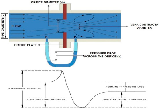
Figure 1.
Orifice meter flow lines and their pressure characteristics.
The pressure difference is computed by calculating the static pressure before and after the minimum limit. The flow rate to the tank can be calculated using Equation (1) [1].
The coefficient of discharge (Cd) is set to 0.8 [48], and A0 denotes the orifice’s cross-sectional area. The static differential pressure at distances of ‘D’ and ‘0.5D’ is represented by (P1 − P2), and the liquid density is denoted by ‘ρ’. The fluid flows through a pipe into a rectangular tank with dimensions ‘L’ of 24 cm and ‘W’ of 30 cm, as illustrated in Figure 2. By keeping the outflow from the tank constant at Q′ = 0.00035 m3/s, the fluid level is measured for various inlet velocities. The initial velocity is incremented by 0.03 m/s every 100 s (step size) until the input velocity increases from 0.03 m/s to 0.6 m/s. To accomplish this, a User-Defined Function (UDF) has been defined for a change in inlet velocity. UDFs are written using a text editor and the C programming language. Equation (2) calculates accumulation when the tank is filled at a flow rate of Q m3/s with a constant outflow rate of Q′ m3/s.
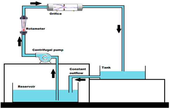
Figure 2.
Experimental setup.
From Equations (2) and (3):
Substituting all the values in Equation (4), we obtain the theoretical liquid level in the tank. A dynamical system is a set of ordinary differential equations of the form shown in Equation (5).
Here, x = (x1, x2, x3,…, xn) ϵ Rn are state variables, and (c1, c2, c3, …, ck) ϵ Rn are control parameters. Using system identification, the MISO system is built for the data obtained from ANSYS, i.e., inlet velocity, temperature, density, and placement at 15 inches, 20 inches, and 25 inches from the pipe inlet.
3.2. System Identification
This is used to identify the model for time and frequency domain data. It is a mathematical model based on observed data from a dynamic system. An active system responds to inputs based on previous data. Mathematical models are becoming increasingly significant in research and engineering. They solve various tasks, such as simulation and control design. Therefore, it is essential to master multiple techniques for model building. There are two approaches to modeling a dynamic system:
- First-principles model
- Data-driven model
In this work, the data from CFD modeling are subsequently loaded into SIT for system identification, i.e., gray box modeling.
The state–space model of the system is represented as shown in Equation (6):
where x(t) is the state vector, u(t) is the input vector, and y(t) is the output vector. The constant matrices A, B, C, and D are computed using the system identification toolbox as mentioned.
4. Design of the Estimator
4.1. Design of the Lorenz Estimator
The Lorenz equation is a three-dimensional, nonlinear system of differential equations [49]. It consists of three variables/initial conditions, x1, x2, and x3, at time t. The Lorenz equation has three real positive parameters: sigma (σ), rho (ρ), and beta (β), where σ is the Prandtl number, ρ is the Rayleigh number, and β is some physical proportion of the region under consideration. The parameter values σ > 0, ρ > 0, and β > 0 cause a system to be chaotic [50]. For a given initial condition (x1, x2, and x3), the future path of this point is determined using Equation (7). These equations show how the variables interact with each other and how the variables change over time [27].
Variables and in Equation (7) involve quadratic nonlinearities. The intensity of the fluid motion is parameterized by the variables x1, x2, and x3, where x1 is the inlet velocity, x2 is the liquid temperature, and x3 is the liquid density. Long-term prediction becomes difficult without knowledge of the initial conditions. Lyapunov exponents characterize the quantities of dynamical systems. The maximal Lyapunov exponent (MLE) estimates the scale of the chaos. It calculates the average rate at which the system’s predictability deteriorates. The Lorenz equations contain three Lyapunov exponents, with motion in x1, x2, and x3. For the system to be chaotic, a positive MLE is considered. The Lyapunov exponents are the eigenvalues of the Jacobian at critical values. Solutions to Lorenz equations lead to chaos or nonchaos based on parameters σ, β, and ρ. For this, critical points need to be determined. These critical points for the Lorenz equations mentioned in Equation (7) are (0, 0, 0). For chaotic behavior with a critical point (0, 0, 0), ρ < 1. For the other two critical points, ρ > 1. The solutions will reach fixed points if we start close to these critical points. Therefore, the Lyapunov exponents of the chaotic system at these critical points need to be determined. The Lyapunov exponents are the eigenvalues of the Jacobian matrix. The Jacobian matrix of the Lorenz system at the critical point (0, 0, 0) is mentioned in Equation (8).
It has the characteristic polynomial:
Eigenvalues are the roots of this polynomial:
For the parameter values of σ = 10, β = 8/3, and ρ = 0.5, the solution depends sensitively on the initial conditions and exhibits chaotic behavior [6]. Therefore, using these parameters, we obtain (−8/3, −10.5249, −0.4751) as eigenvalues for critical points (0, 0, 0). For the critical points , i.e., (8.4853, 8.4853, 27), with the parameters σ = 10, β = 8/3, and ρ = 28, the eigenvalues are computed as (−13.8546, 0.094 − 10.1945j, 0.094 + 10.1945j). The estimator results in an infinite solution for the critical points (8.4853, 8.4853, 27). Hence, the parameters for the design of the estimator are chosen to be σ = 10, β = 8/3, and ρ = 0.5. The constant matrices A, B, C, and D for a Lorenz estimator are shown above. The chaotic estimator is designed using the Jacobian matrix obtained from the Lorenz equations for the above system.
Since the constant matrix is , the output is y = . The constant gain matrix is computed as follows:
4.2. Design of the Rossler Estimator
Being deterministic, Lorenz equations have no random noise or stochastic terms and determine a unique flow. ‘Rossler’ is a continuous, chaotic system. A study on the dynamics of the Rossler ODEs (ordinary differential equations) is investigated in ref. [51]. The Rossler equation [52] has three nonlinear differential equations that can generate chaotic behavior under certain conditions defined by Equation (11). This equation has only one nonlinear term ().
These differential equations characterize a continuous-time dynamical system with chaotic dynamics linked to the attractor’s fractal properties. Chaotic behavior is the desired outcome of choosing a = b = 0.2 and c = 5.7 for the system. The constant matrices A, B, C, and D for a Rossler estimator are shown above.
The Jacobian matrix for Equation (11) is defined in Equation (12).
The critical points for these parameters are calculated to be:
Hence,
For these critical points, the eigenvalues are calculated to be:
The feedback gain matrix is computed as follows:
The system exhibits chaotic behavior as it is nonlinear and takes initial conditions into account. The solution of the nonlinear differential equation of Lorenz and Rossler is plotted for two different initial conditions [53] to observe the system sensitivity to the initial conditions. The SIMULINK model of the plant with the estimator is shown in Figure 3. The overall process involved in liquid level estimation using the Lorenz and Rossler estimators is described in Figure 4.
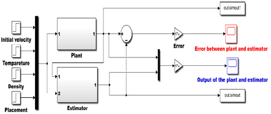
Figure 3.
Simulink model of the system with the estimator.
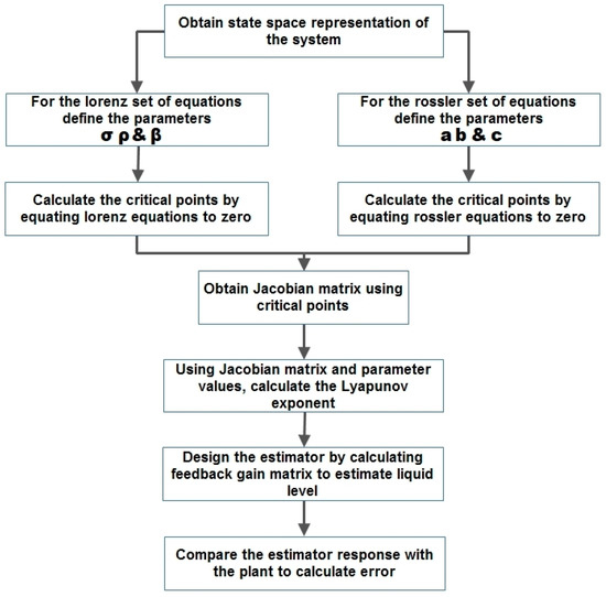
Figure 4.
Flow chart for designing the estimator.
The observer aims to estimate the true state x(t). It is acceptable to expect some error in the estimate initially, but the aim is for the error to reduce over time. The estimation error is calculated using Equation (13):
Consequently, the homogeneous differential equation governing the state of the estimation error is determined by the n × n matrix A-LC. The estimated error gradually approaches zero by choosing the gain matrix L so that the eigenvalues of A-LC are located exclusively in the left half of the complex plane, hence asymptotically stabilizing the error equation. The eigenvalues of A-LC can be located anywhere in the plane when the system (A, C) is completely observable, with the restriction that complex eigenvalues can only exist in complex conjugate pairs. As (A, C) is detectable, selecting L can render A-LC asymptotically stable. Integrating state–space modeling of the system with these chaotic observers makes them highly sensitive to small changes in the system, making them effective in tracking and estimating the system’s state.
4.3. Prediction Using the ANN Model
ANNs are a type of machine learning algorithm that is widely used for classification and prediction tasks. Neural networks are designed to emulate the functioning of biological neural networks. ANNs consist of multiple layers of artificial neurons arranged in a network-like structure. The typical structure of an ANN includes an input layer, one or more hidden layers, and an output layer. The input layer receives the data that need to be processed, while the output layer produces the final result of the computation. The hidden layers perform intermediate computations on the data, transforming them through a series of nonlinear transformations. Each layer in an ANN is composed of multiple artificial neurons, also called nodes. These nodes are interconnected, and their interactions are determined by the weights assigned to their connections. The weights represent the strength of the connections between the nodes, and they are adjusted during the training process of the ANN to improve its accuracy. Figure 5 shows the architecture of an ANN, where the artificial neurons in one layer are connected to those in the next layer through weights. The number of nodes in each layer and the number of layers can vary depending on the complexity of the problem at hand. ANNs have been successfully applied in various fields, including computer vision, natural language processing, and finance.
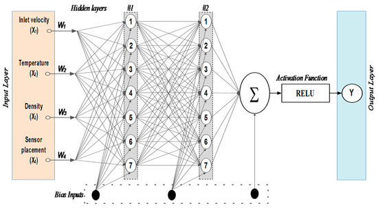
Figure 5.
Architecture of an artificial neural network.
In this work, an ANN is used to design a mathematical model of the observations so that predictions can be made [54]. Figure 5 explains the model of the ANN, which is built to predict liquid height in a tank. ‘X’ is the input parameter, and ‘Y’ is the fluid level. Normalized output data using standard scaling are used for supervised learning with the output data obtained from ANSYS. Hyperparameter searching determines the total number of parameters (weights and biases). The trained model is tested for its accuracy and MSE. The liquid level is estimated with an optimization algorithm that gives the least MSE. The complete details are described below.
To build an ANN model, the following four steps are typically employed:
- Supervised learning requires selecting appropriate input and output data.
- Input data normalization is performed to ensure the data are within a consistent range.
- The model is trained on the normalized data using hyperparameter searching, which involves adjusting the model parameters to optimize its performance.
- The model’s goodness of fit is assessed through testing.
In addition, the predicted output is compared with the actual output to evaluate the model’s performance. By following these steps, an ANN model can be built and refined to improve its accuracy in making predictions or classifications.
4.3.1. Selection of the Input and Output Data for the Supervised Learning
Pandas loads simulated data from ANSYS into a data frame. The vectors of inflow velocity, temperature, density, and sensor location make up the input data in this case. The height of the fluid in the tank makes up the output vector.
4.3.2. Normalization of Input and Output Data
The imported data are normalized because their units and ranges are mismatched. This prevents the values of the input and output from not correlating with one another.
4.3.3. Training of the Normalized Data and Building the Model Using Hyperparameter Searching
The model uses a neural network with two to three hidden layers. In each hidden layer, the number of neurons ranges from six to eight in one increment. Within the model, a random search is performed to determine the best possible neural network. An activation function is a critical component of an ANN that helps generate output from a collection of input values provided to the node (or layer). In neural networks, there are three activation functions: binary step activation, linear activation, and complex nonlinear activation functions. The rectified linear unit (ReLU) activation function was used in this case. The primary purpose of employing the ReLU activation function, a nonlinear neural network activation function, is to solve the vanishing gradient issues when numerous hidden layers exist in the network. It also enables the model to learn quickly and perform better than the other two activation functions. Equation (14) represents the mathematical equation for ReLU.
In this case, the ReLU’s output is “0” for negative inputs and “x” for positive values. Optimizers are algorithms or techniques that change a neural network’s parameters, including weights and learning rates, to minimize losses. Optimizers address optimization issues by reducing the function. Since the Adam optimizer yields a minimum mean squared error (MSE) of 1.1638 × 10⁻⁶, it is utilized for compilation. In this case, the learning rate is a hyperparameter value. Based on a random search, the optimal learning rate is selected among 0.001, 0.0001, and 0.00001. After 50 iterations, the model is trained.
4.3.4. Testing the Goodness of Fit of the Model
Testing is conducted after the data training is finished and the error is below the tolerance criteria. The MSE value measures the goodness of fit of the best model selected, as mentioned in Section 4.3.3.
4.3.5. Comparison of Actual Data and Predicted Data
Once testing is complete, the results are plotted between the actual output and the predicted output to make a comparison. Predicted and desired height values are plotted for inlet velocity 0.6 m/s, temperature 50 °C, and density 900 kg/m3 and placed 20 inches from the inlet. In ref. [33], it was reported that ANNs with fewer hidden layers can achieve the same level of training performance compared to a higher number of hidden layers. This simplification of the ANN architecture improves the hardware implementation performance. In this report, training was performed for two different numbers of hidden layers, 2 and 14, which gives MSEs of 1.1638 × and 1.0989 × , respectively, as tabulated in Table 1. It can be concluded that the minor increase in MSE can be a fair trade-off, knowing that the lesser hidden layer has many benefits:

Table 1.
Level estimation for different parameters when the sensor is placed 20 inches from the inlet.
- A smaller hidden layer means fewer neurons, reducing the ANN architecture’s complexity and hardware utilization.
- This reduces the computational cost.
- A large number of samples increases the time consumed for training the ANN.
This work used the ANN architecture of two layers for validation purposes.
5. Results and Discussion
As seen in Figure 6, a pressure sensor (orifice) is attached to a panel held vertically for validation. Place the orifice plate in the piping system downstream of the control valve. The flow bypass manual valve can be opened or closed to change the flow rate. The flow rate in LPH is measured with a rotameter. As liquid flows through the pressure sensor, it gathers underneath the tank. Equation (15) represents the conversion of the flow rate to the inlet velocity.
Flowrate (Q) = Inlet velocity (V) × Cross sectional area (A)
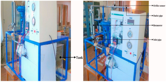
Figure 6.
Practical setup.
The level is estimated using the tank size and the volume obtained. The equation essentially expresses that the velocity of the liquid at the inlet is the flow rate divided by the cross-sectional area. This relationship helps to understand the speed at which the liquid is entering the system. The level estimation for different parameters when the sensor is placed at a particular location from the inlet is shown in Table 2. The entire methodology workflow is shown in Figure 7.

Table 2.
Model summary.
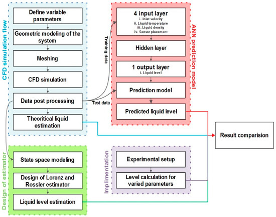
Figure 7.
The workflow of CFD simulation, design of the estimator, ANN prediction model, and real-time implementation.
The Lorenz equations with parameters σ = 10, ρ = 0.5, and β = 8/3 are used for designing the chaotic estimator to estimate the height of the liquid in the tank. For the state–space model obtained from system identification, the fit to estimation data is 92.18%, and the final prediction error is 2.64 × 10⁻⁵. The output is chosen as y = x1, i.e., C = . Initial conditions are chosen as x(0) = 0.02, y(0) = 0.1, and z(0) = 0.1. The resulting estimation of the liquid level for the inlet velocity = 0.6 m/s, temperature = 50 °C, density = 900 kg/m3, and a sensor placed 20 inches from the inlet are shown in Figure 8. The error between the system and the estimator response is plotted in Figure 9.
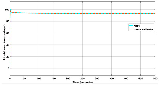
Figure 8.
Liquid level estimation with the initial condition (0.02, 0.1, 0.1) using the Lorenz estimator.
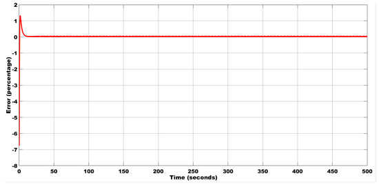
Figure 9.
Error estimation between the plant and the estimator with the initial condition (0.02, 0.1, 0.1) using the Lorenz estimator.
To incorporate the effect of the initial condition, the response is obtained by having a slight change in the initial condition, i.e., x(0) = 0.025, y(0) = 0.15, and z(0) = 0.15. The corresponding estimations of the liquid level and error are plotted in Figure 10 and Figure 11, respectively.
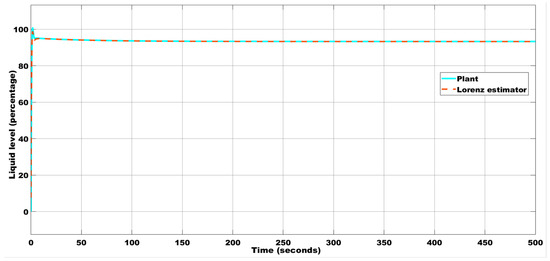
Figure 10.
Liquid level estimation with the initial condition (0.025, 0.15, 0.15) using the Lorenz estimator.
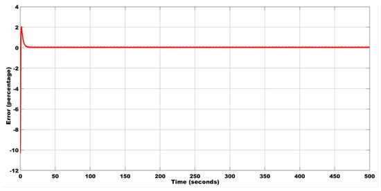
Figure 11.
Error estimation between the plant and the Lorenz estimator with the initial condition (0.025, 0.15, 0.15) using the Lorenz estimator.
To check the system’s robustness to noise, a disturbance signal of amplitude 10−6 is added, and the estimation of the liquid level and error are plotted in Figure 12 and Figure 13, respectively. Using the Rossler estimator, with the initial conditions of x(0) = 0.02, y(0) = 0.1, and z(0) = 0.1, the estimation of the liquid level for the inlet velocity = 0.6 m/s, temperature = 50 °C, density = 900 kg/m3, and having the sensor placed 20 inches from the inlet is shown in Figure 14. The error between the system and the estimator response is plotted in Figure 15.
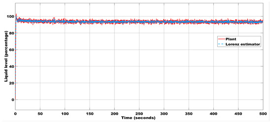
Figure 12.
Liquid level estimation with the initial condition (0.02, 0.1, 0.1) using the Lorenz estimator with a noise magnitude of 10−6.
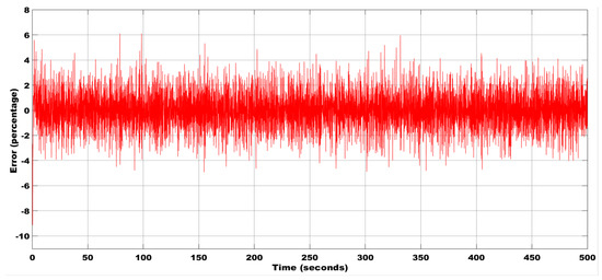
Figure 13.
Error estimation between the plant and the Lorenz estimator with the initial condition (0.02, 0.1, 0.1) using the Lorenz estimator.
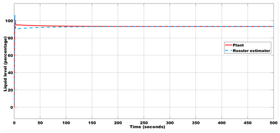
Figure 14.
Liquid level estimation with the initial condition (0.02, 0.1, 0.1) using the Rossler estimator.
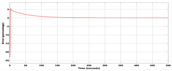
Figure 15.
Error estimation between the plant and the estimator with the initial condition (0.02, 0.1, 0.1) using the Rossler estimator.
To incorporate the effect of initial conditions, the response is obtained by having a slight change in the initial condition, i.e., x(0) = 0.025, y(0) = 0.15, and z(0) = 0.15. The corresponding liquid level and error estimations are plotted in Figure 16 and Figure 17, respectively. To check the system’s robustness to noise, a disturbance signal of amplitude 10−6 is added, and the estimation of the liquid level and error are plotted in Figure 18 and Figure 19, respectively.
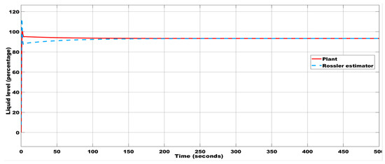
Figure 16.
The liquid level estimation with the initial condition (0.025, 0.15, 0.15) using the Rossler estimator.
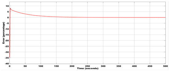
Figure 17.
Error estimation between the plant and the estimator with the initial condition (0.025, 0.15, 0.15) using the Rossler estimator.
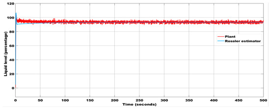
Figure 18.
Liquid level estimation with the initial condition (0.02, 0.1, 0.1) using the Rossler estimator with a noise magnitude of 10−6.
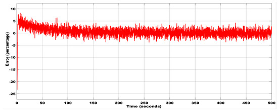
Figure 19.
The noise between the plant and the estimator with the initial condition (0.02, 0.1, 0.1) using the Rossler estimator.
For these different initial conditions and parameter values, with inlet velocity = 0.6 m/s, temperature = 50 °C, density = 900 kg/m3, and sensor placement at 20 inches from the pipe inlet, the MSEs are computed. They are found to be less, as shown in Table 3.

Table 3.
Calculation of the mean squared error.
In general, density can be altered by adjusting the pressure or the temperature. Constantly increasing the pressure causes a material’s density to rise. In most circumstances, increasing the temperature causes the density to decrease. To decrease the density below water, i.e., below 998 kg/m3, acetone, a chemical substance, is used as a low-density liquid. The acetone density is 0.788 g/mL, or 780 kg/m3, at room temperature. Since it dissolves in water, mixing it with the water can alter the density to the needed amount. The density is kept at approximately 900 kg/m3 for validation purposes. Since it evaporates quickly and is flammable, experimentation is conducted at room temperature, i.e., 28 °C, and the results are as expected. The physical system estimation method in Table 4 was performed for acetone, keeping density at 900 kg/m3 and temperature at approximately 50 °C since the boiling point of acetone is 56 °C.

Table 4.
Comparison of the liquid level in the tank using various methods for given input parameters.
For the observed data, the prediction model is generated using an ANN. The observed data are preprocessed and imported using the ‘Pandas’ data frame. As the independent variables have different ranges, they are normalized using conventional scaling before being subdivided into test and train data. The ANN model has four input layers and one output layer. The activation function is a rectified linear activation function known as ReLU. The performance metric, mean squared error, is calculated using several optimization strategies. Figure 20 depicts the prediction result after running the model for 50 epochs and testing it with test data.
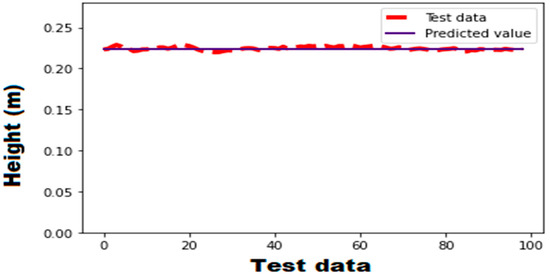
Figure 20.
Prediction for inlet velocity, y = 0.6 m/s, temperature = 50 °C, density = 900 kg/m3, and placement of the sensor at 20 inches from the pipe inlet using an ANN.
Likewise, the model is used for various optimization functions. The loss functions are plotted for 50 epochs, as shown in Figure 21. Since the Adam optimizer results in the least MSE, the same is chosen for prediction.
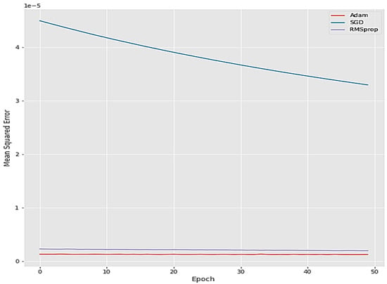
Figure 21.
Loss functions for 50 epochs.
6. Conclusions
This paper discusses how to estimate the fluid level in a tank. The laminar type of water flow through an orifice meter with a fixed pipe length and orifice diameter is investigated using a CFD simulation. The flow rate is calculated for various inflow velocities, temperatures, densities, and sensor locations. The Lorenz and Rossler estimators are both designed for the same system. The results obtained are additionally verified using an ANN prediction model. The height of the liquid is expected to be correct for an input velocity of 0.6 m/s, a temperature of 50 °C, a liquid density of 900 kg/m3, and a sensor situated 20 inches from the intake of the pipe, as shown in Table 3. To reduce the inaccuracy, many optimization strategies are applied. Table 2 shows that the computed MSE is the smallest. Actual data, simulated values, and estimated values are compared using the experimental setup, and the liquid level is shown to be correct. The error percentage is estimated depending on whether or not there are problems in the system and is lower than 6%. These virtual sensors are computational algorithms that estimate or predict process variables or conditions using available measurements and models. They find applications in various industries due to their ability to provide valuable information in situations where direct measurements may be challenging or expensive. They contribute to increased efficiency, reduced costs, and improved process control across various industries, making them valuable tools in complex and dynamic systems. These chaotic observers can be used in synchronization schemes, where the observer synchronizes its chaotic behavior with the target system. This is employed in secure communication, cryptography, and certain control applications.
Author Contributions
Conceptualization, V.S. and S.K.V.; methodology, V.S. and P.S.; software, V.S. and P.S.; validation, S.K.V., V.S. and P.S.; formal analysis, V.S. and P.S.; investigation, S.K.V.; resources, V.S.; data curation, V.S.; writing—original draft preparation, V.S.; writing—review and editing, S.K.V. and P.S.; visualization, V.S.; supervision, S.K.V.; project administration, S.K.V. All authors have read and agreed to the published version of the manuscript.
Funding
This research received no external funding.
Data Availability Statement
All data generated or analyzed during this study are included in this article.
Conflicts of Interest
The authors declare no conflicts of interest.
References
- Shah, M.S.; Joshi, J.B.; Kalsi, A.S.; Prasad, C.; Shukla, D.S. Analysis of flow through an orifice meter: CFD simulation. Chem. Eng. Sci. 2012, 71, 300–309. [Google Scholar] [CrossRef]
- Xu, H.; Ding, F.; Sheng, J. On some parameter estimation algorithms for the nonlinear exponential autoregressive model. Int. J. Adapt. Control Signal Process. 2019, 33, 999–1015. [Google Scholar] [CrossRef]
- Gershenson, C. Artificial Neural Networks for Beginners. arXiv 2003. [Google Scholar] [CrossRef]
- Kv, S.; Nair, N.; Nayak, S. Analysis of Propagation of Errors Due to Sensor Faults in a Flow Process for Design of Fault Isolation. In Proceedings of the 2018 2nd International Conference on Power, Energy and Environment: Towards Smart Technology (ICEPE), Shillong, India, 1–2 June 2018; pp. 1–5. [Google Scholar] [CrossRef]
- Singh, P.P. A Chaotic System with Large Lyapunov Exponent: Nonlinear Observer Design and Circuit Implementation. In Proceedings of the 2020 3rd International Conference on Energy, Power and Environment: Towards Clean Energy Technologies, Shillong, Meghalaya, India, 5–7 March 2021; pp. 1–6. [Google Scholar] [CrossRef]
- Wiggins, S. (Ed.) Hamiltonian Vector Fields. In Introduction to Applied Nonlinear Dynamical Systems and Chaos, in Texts in Applied Mathematics; Springer: New York, NY, USA, 2003; pp. 197–230. [Google Scholar] [CrossRef]
- Ann, N.Q.; Pebrianti, D.; Abas, M.F.; Bayuaji, L.; Syafrullah, M. Parameter Prediction for Lorenz Attractor by using Deep Neural Network. Indones. J. Electr. Eng. Inform. (IJEEI) 2020, 8, 532–540. [Google Scholar] [CrossRef]
- Li, Y. A Kind of Nonlinear Observer Design. In Proceedings of the 2020 Chinese Automation Congress (CAC), Shanghai, China, 6–8 November 2020; pp. 2014–2016. [Google Scholar] [CrossRef]
- Aksoy, A.; Zhang, F.; Nielsen-Gammon, J.W. Ensemble-Based Simultaneous State and Parameter Estimation in a Two-Dimensional Sea-Breeze Model. Mon. Weather. Rev. 2006, 134, 2951–2970. [Google Scholar] [CrossRef][Green Version]
- Nathasarma, R.; Roy, B.K. Physics-Informed Long-Short-Term Memory Neural Network for Parameters Estimation of Nonlinear Systems. IEEE Trans. Ind. Appl. 2023, 59, 5376–5384. [Google Scholar] [CrossRef]
- Kvarda, P. Identifying the Deterministic Chaos by Using the Lyapunov Exponents. June 2001. Available online: http://dspace.vutbr.cz/handle/11012/58190 (accessed on 27 November 2023).
- Kaplan, J.L.; Yorke, J.A. Preturbulence: A regime observed in a fluid flow model of Lorenz. Commun. Math. Phys. 1979, 67, 93–108. [Google Scholar] [CrossRef]
- Kutz, J.N. Data-Driven Modeling & Scientific Computation: Methods for Complex Systems & Big Data; OUP Oxford: Oxford, UK, 2013. [Google Scholar]
- Brunton, S.L.; Noack, B.R.; Koumoutsakos, P. Machine Learning for Fluid Mechanics. Annu. Rev. Fluid Mech. 2020, 52, 477–508. [Google Scholar] [CrossRef]
- Erichson, N.B.; Mathelin, L.; Yao, Z.; Brunton, S.L.; Mahoney, M.W.; Kutz, J.N. Shallow neural networks for fluid flow reconstruction with limited sensors. Proc. R. Soc. A Math. Phys. Eng. Sci. 2020, 476, 20200097. [Google Scholar] [CrossRef] [PubMed]
- Mata-Machuca, J.L.; Martínez-Guerra, R.; Aguilar-López, R. Chaotic Systems Synchronization Via High Order Observer Design. J. Appl. Res. Technol. 2011, 9, 57–68. [Google Scholar] [CrossRef]
- Hato, E.; Shihab, D. Lorenz and Rossler Chaotic System for Speech Signal Encryption. Int. J. Comput. Appl. 2015, 128, 25–33. [Google Scholar] [CrossRef]
- Liu, Y.; Davis, P. Dual synchronization of chaos. Phys. Rev. E 2000, 61, R2176–R2179. [Google Scholar] [CrossRef]
- Ning, D.; Lu, J.-A.; Han, X. Dual synchronization based on two different chaotic systems: Lorenz systems and Rössler systems. J. Comput. Appl. Math. 2007, 206, 1046–1050. [Google Scholar] [CrossRef]
- Alsafasfeh, Q.H.; Al-Arni, M.S. A New Chaotic Behavior from Lorenz and Rossler Systems and Its Electronic Circuit Implementation. Circuits Syst. 2011, 2, 101–105. [Google Scholar] [CrossRef]
- Liang, X.; Zhang, J.; Xia, X. Adaptive synchronization for generalized Lorenz systems. IEEE Trans. Autom. Control 2008, 53, 1740–1746. [Google Scholar] [CrossRef][Green Version]
- Wang, X.; Jiang, F.; Yin, J. Existence and Uniqueness of the Solution of Lorentz-Rössler Systems with Random Perturbations. Abstr. Appl. Anal. 2013, 2013, e480259. [Google Scholar] [CrossRef]
- Ibrahim, K.M.; Jamal, R.K.; Ali, F.H. Chaotic behaviour of the Rossler model and its analysis by using bifurcations of limit cycles and chaotic attractors. J. Phys. Conf. Ser. 2018, 1003, 012099. [Google Scholar] [CrossRef]
- Morgül, Ö.; Solak, E. Observer based synchronization of chaotic systems. Phys. Rev. E 1996, 54, 4803–4811. [Google Scholar] [CrossRef] [PubMed]
- Awodele, O.; Jegede, O. Neural Networks and Its Application in Engineering. In Proceedings of the InSITE 2009: Informing Science + IT Education Conference, Macon, GA, USA, 12–15 June 2009; Volume 9. Available online: https://www.informingscience.org/Publications/3317 (accessed on 27 November 2023).
- Dubois, P.; Gomez, T.; Planckaert, L.; Perret, L. Data-driven predictions of the Lorenz system. Phys. D Nonlinear Phenom. 2020, 408, 132495. [Google Scholar] [CrossRef]
- Morgül, Ö.; Solak, E. On the Synchronization of Chaos Systems by Using State Observers. Int. J. Bifurc. Chaos 1997, 7, 1307–1322. [Google Scholar] [CrossRef]
- Shenoy, V.; Santhosh, K.V. Design Of Estimator For Level Monitoring Using Data Driven Model. In Proceedings of the 2021 2nd International Conference on Computation, Automation and Knowledge Management (ICCAKM), Dubai, United Arab Emirate, 19–21 January 2021; pp. 81–86. [Google Scholar] [CrossRef]
- Sun, Y.-J. A simple observer design of the generalized Lorenz chaotic systems. Phys. Lett. A 2010, 374, 933–937. [Google Scholar] [CrossRef]
- Barrio, R.; Serrano, S. A three-parametric study of the Lorenz model. Phys. D Nonlinear Phenom. 2007, 229, 43–51. [Google Scholar] [CrossRef]
- Barrio, R.; Serrano, S. Bounds for the chaotic region in the Lorenz model. Phys. D Nonlinear Phenom. 2009, 238, 1615–1624. [Google Scholar] [CrossRef]
- Torres-Treviño, L.; Rodriguez, A. Parameter Estimation Based on Evolutionary Computation for P-Class Chaotic Systems. IFAC Proc. Vol. 2012, 45, 170–174. [Google Scholar] [CrossRef]
- He, W.-P.; Wang, L.; Jiang, Y.-D.; Wan, S.-Q. An improved method for nonlinear parameter estimation: A case study of the Rössler model. Theor. Appl. Clim. 2016, 125, 521–528. [Google Scholar] [CrossRef]
- Annan, J.D.; Hargreaves, J.C. Efficient parameter estimation for a highly chaotic system. Tellus A Dyn. Meteorol. Oceanogr. 2004, 56, 520–526. [Google Scholar] [CrossRef]
- Liao, T.-L.; Huang, N.-S. An observer-based approach for chaotic synchronization with applications to secure communications. IEEE Trans. Circuits Syst. I Regul. Pap. 1999, 46, 1144–1150. [Google Scholar] [CrossRef]
- Zhang, L. Artificial Neural Network Architecture Design for EEG Time Series Simulation Using Chaotic System. In Proceedings of the 2018 Joint 7th International Conference on Informatics, Electronics & Vision (ICIEV) and 2018 2nd International Conference on Imaging, Vision & Pattern Recognition (icIVPR), Kitakyushu, Japan, 25–29 June 2018; pp. 388–393. [Google Scholar] [CrossRef]
- Ukpaka, C.P.; Ukpaka, C. Model prediction for constant area, variable pressure drop in orifice plate characteristics in flow system. Chem. Int. 2022, 2, 80–88. [Google Scholar]
- Monjardin, C.E.F.; Uy, F.A.A.; Tan, F.J.; Cruz, F.R.G. Automated Real-time Monitoring System (ARMS) of hydrological parameters for Ambuklao, Binga and San Roque dams cascade in Luzon Island, Philippines. In Proceedings of the 2017 IEEE Conference on Technologies for Sustainability (SusTech), Phoenix, AZ, USA, 12–14 November 2017; pp. 1–7. [Google Scholar] [CrossRef]
- Cruz, F.R.G.; Binag, M.G.; Ga, M.R.G.; Uy, F.A.A. Flood Prediction Using Multi-Layer Artificial Neural Network in Monitoring System with Rain Gauge, Water Level, Soil Moisture Sensors. In Proceedings of the TENCON 2018—2018 IEEE Region 10 Conference, Jeju, Republic of Korea, 28–31 October 2018; pp. 2499–2503. [Google Scholar] [CrossRef]
- Bhar, K.K.; Bakshi, S. Application of artificial neural network for predicting water levels in Hooghly estuary, India. H2Open J. 2020, 3, 401–415. [Google Scholar] [CrossRef]
- Bustami, R. Artificial neural network for precipitation and water level predictions of bedup river. IAENG Int. J. Comput. Sci. 2007, 34, 2. Available online: https://www.academia.edu/24753916/Artificial_neural_network_for_precipitation_and_water_level_predictions_of_bedup_river (accessed on 27 November 2023).
- Chegini, H.G.; Zarepour, G. Utilizing Artificial Neural Network for Load Prediction Caused by Fluid Sloshing in Tanks. Geofluids 2021, 2021, e3537542. [Google Scholar] [CrossRef]
- Liu, C.-H.; Yang, T.-H.; Wijaya, O.T. Development of an Artificial Neural Network Algorithm Embedded in an On-Site Sensor for Water Level Forecasting. Sensors 2022, 22, 8532. [Google Scholar] [CrossRef]
- Nathasarma, R.; Roy, B.K. Parameter estimation of nonlinear systems with stable, chaotic and periodic behaviours at different initial conditions—A new approach. In Proceedings of the 2022 4th International Conference on Energy, Power and Environment (ICEPE), Shillong, India, 29 April–1 May 2022; pp. 1–6. [Google Scholar] [CrossRef]
- Shenoy, V.; Kv, S. Characterization of orifice performance using Computational Fluid Dynamics. In Proceedings of the 2021 IEEE Mysore Sub Section International Conference (MysuruCon), Hassan, India, 24–25 October 2021; pp. 87–91. [Google Scholar] [CrossRef]
- Kojasoy, G.; Landis, F.; Kwame-Mensah, P.; Chang, C. Two-phase pressure drop in multiple thick- and thin-orifice plates. Exp. Therm. Fluid Sci. 1997, 15, 347–358. [Google Scholar] [CrossRef]
- Tukiman, M.M.; Ghazali, M.N.M.; Sadikin, A.; Nasir, N.F.; Nordin, N.; Sapit, A.; Razali, M.A. CFD simulation of flow through an orifice plate. IOP Conf. Ser. Mater. Sci. Eng. 2017, 243, 012036. [Google Scholar] [CrossRef]
- Reader-Harris, M.J. Computation of Flow through Orifice Plates. 1989, Volume 6, pp. 1907–1917. Available online: https://ui.adsabs.harvard.edu/abs/1989nmlt.conf.1907R (accessed on 27 November 2023).
- Peng, C.-C.; Li, Y.-R. Parameters identification of nonlinear Lorenz chaotic system for high-precision model reference synchronization. Nonlinear Dyn. 2022, 108, 1733–1754. [Google Scholar] [CrossRef]
- Lorenz, E.N. Deterministic Nonperiodic Flow. J. Atmos. Sci. 1963, 20, 130–141. [Google Scholar] [CrossRef]
- Barrio, R.; Blesa, F.; Dena, A.; Serrano, S. Qualitative and numerical analysis of the Rössler model: Bifurcations of equilibria. Comput. Math. Appl. 2011, 62, 4140–4150. [Google Scholar] [CrossRef][Green Version]
- Rössler, O. An equation for continuous chaos. Phys. Lett. A 1976, 57, 397–398. [Google Scholar] [CrossRef]
- Sahoo, A.K.; Udgata, S.K. A Novel ANN-Based Adaptive Ultrasonic Measurement System for Accurate Water Level Monitoring. IEEE Trans. Instrum. Meas. 2020, 69, 3359–3369. [Google Scholar] [CrossRef]
- Chen, L.; Zhu, Y.; Ahn, C.K. Adaptive Neural Network-Based Observer Design for Switched Systems with Quantized Measurements. IEEE Trans. Neural Netw. Learn. Syst. 2023, 34, 5897–5910. [Google Scholar] [CrossRef]
Disclaimer/Publisher’s Note: The statements, opinions and data contained in all publications are solely those of the individual author(s) and contributor(s) and not of MDPI and/or the editor(s). MDPI and/or the editor(s) disclaim responsibility for any injury to people or property resulting from any ideas, methods, instructions or products referred to in the content. |
© 2024 by the authors. Licensee MDPI, Basel, Switzerland. This article is an open access article distributed under the terms and conditions of the Creative Commons Attribution (CC BY) license (https://creativecommons.org/licenses/by/4.0/).