Assessing the Impact of Psyllid Pesticide Resistance on the Spread of Citrus Huanglongbing and Its Ecological Paradox

Abstract

Excessive use of pesticides can lead to pesticide resistance in citrus psyllids, and studies have shown that this resistance is related to population genetics. This article proposes a dynamic model of Huanglongbing (HLB) that integrates the population genetics of the citrus psyllid vector and considers the fitness cost associated with pesticide resistance to study how pesticide use affects the development of pesticide resistance at the population level. The basic reproduction number is introduced as a metric to assess whether HLB can be effectively controlled. Additionally, this article explores the impact of different parameters on the spread of HLB. Numerical simulations illustrate that the basic reproduction number decreases as the fitness cost of resistance increases, while an increase in the resistance index leads to an increase in the basic reproduction number. However, when the fitness cost is sufficiently high, a larger resistance index may result in a basic reproduction number less than 1, leading to the extinction of Asian citrus psyllid (ACP), thus causing a paradox effect.

1. Introduction

Citrus Huanglongbing (HLB), caused by the bacterium Candidatus Liberibacter asiaticus, is a devastating disease that affects citrus plants. HLB leads to irregular yellowing of leaves, reduced fruit production, uneven fruit coloring, and damage to the plant’s root system. In severe cases, it can even result in the death of the trees. When the incidence of HLB in an orchard exceeds 5%, the disease can rapidly spread through transmission by the Asian citrus psyllid, often leading to the destruction of all citrus trees in the orchard within 8 to 10 years.

The Asian citrus psyllid is the sole natural vector for the transmission of HLB [1]. Infected psyllids carry the HLB pathogen and transmit it to healthy citrus trees by feeding on their sap, resulting in the healthy trees becoming infected. Conversely, healthy psyllids can become carriers of the pathogen by feeding on infected citrus trees [2]. Consequently, the infection between citrus trees and psyllids is mutual, and once a citrus tree is infected with HLB, it cannot be cured [3].

To date, due to the absence of resistant varieties and curative methods, the primary focus in managing HLB is controlling the Asian citrus psyllid (ACP). Among the various control measures, chemical control—specifically spraying insecticides—is the most commonly employed method [4]. While chemical methods are effective in preventing and controlling the spread of HLB, prolonged and extensive use of insecticides can result in numerous issues, such as excessive pesticide residues, environmental harm, and loss of biodiversity. Recent studies have revealed that the ACP has developed varying degrees of resistance to different insecticides, complicating the control of HLB even further [5,6]. Tian et al. [5] assessed the resistance of four field populations to nine different insecticides using a leaf-dip method. The results indicated that, compared to laboratory-susceptible populations, the resistance ratio of the psyllid population in Zengcheng District, Guangzhou, China, was 15.12, with the highest resistance level to imidacloprid. Similarly, Tiwari et al. [6] investigated the insecticide resistance of adult and nymph psyllids in Florida field populations. Their findings showed that ACP populations across Florida’s citrus-growing areas exhibited varying levels of resistance to multiple insecticides. This suggests that without effective resistance management, insecticide resistance could become a significant new challenge in controlling the Asian citrus psyllid.

Research on insecticide resistance is typically divided into three main stages. The first stage involves studying physiological resistance, the second focuses on biochemical mechanisms, and the third examines genetic mechanisms, including genes, chromosomes, and other genetic materials. At the genetic level, resistance development is governed by three primary mechanisms: (1) gene amplification; (2) changes in gene expression; and (3) alterations in gene structure [7]. Tiwari et al. [6,8,9] studied the differences in cytochrome $P_{450}$ (general oxidase) and glutathione transferase (GST) levels in ACPs infected and uninfected with the HLB pathogen, confirming that the sensitivity of psyllids to insecticides is related to the levels of detoxification enzymes in the body. Their results showed that the activity of cytochrome $P_{450}$ oxidase and GST was significantly lower in infected psyllid adults compared to uninfected ones. Additionally, infection with the HLB pathogen alters certain physiological mechanisms within the psyllid, leading to changes in enzyme activity, which further increases the psyllid’s sensitivity to insecticides. Yu and Killiny [10] analyzed the expression levels of three GST genes in psyllids treated with chlorpyrifos, fenpropathrin, and thiamethoxam. The results indicated that the expression of DcGSTd1 and DcGSTe2 genes significantly increased in psyllids treated with cyfluthrin and thiamethoxam, demonstrating that GST genes play an important role in the development of resistance in psyllids.

In recent years, in response to pest resistance, many experts and scholars from various fields have conducted research. Among these efforts, the use of mathematical models to qualitatively and quantitatively study the transmission dynamics under resistance development conditions has received widespread attention from scholars both domestically and internationally. Many scholars have proposed various mathematical models to explore the impact of pest resistance on the control of disease transmission. Liang et al. [11] simulated three pesticide switching methods to determine the most effective spraying frequencies and optimal strategies for pesticide switching across various scenarios. Tang et al. [12] considered an SI model in which the ACP population was divided into susceptible and resistant types, with a focus on graft transmission and the impact of ACP resistance on the spread of HLB. Luo et al. [13] also studied populations consisting of both susceptible and resistant ACP and investigated the optimal control problems of the HLB model by using optimal control theory. As research progresses, the resistance of ACP has increasingly been linked to genetics, with population genetics emerging as a key area of study. This biological field investigates allele and genotype frequencies within populations [14]. Additionally, several models combining population genetics with epidemiological dynamics have been developed. Freeman et al. [15] introduced the Hardy–Weinberg equilibrium, which posits that allele frequencies remain constant over time. Kuniyoshi et al. [16] employed an SIR model to examine a population with a pair of alleles exhibiting complete dominance, influencing mortality rates induced by insecticides. Jemal et al. [17] integrated epidemiology with vector population genetics to evaluate the impact of insecticide resistance in mosquito populations on the dynamics and control of malaria transmission.

The primary objective of this paper is to develop a dynamical model of HLB that incorporates citrus psyllid resistance and integrates the genetic resistance of the psyllid population to insecticides with the infectious disease model. This model aims to investigate the impact of insecticide resistance in psyllids on the overall dynamics of disease transmission. The paper divides the carrier population into three groups based on genotype, each with distinct characteristics represented by different biological parameter values and varying mortality rates. The structure of the paper is as follows: Section 2 describes the construction of the model. Section 3 analyzes the local stability of the disease-free equilibrium point and the global stability of the citrus trees, assuming no disease-induced mortality or removal of infected trees. Section 4 provides a sensitivity analysis of the basic reproduction number. Section 5 focuses on numerical simulations.

2. Materials and Methods

In this paper, the model analyzes the transmission dynamics of HLB between citrus trees and ACPs. Consequently, the citrus tree population, denoted as $N_h\left(t\right)$, is categorized into susceptible citrus trees ($S_h\left(t\right)$) and infected citrus trees ($I_h\left(t\right)$) at any time t. Therefore, $N_h\left(t\right)$ can be expressed as $N_h\left(t\right)=$ $S_h\left(t\right)+$ $I_h\left(t\right)$.

It is noted that insecticide resistance in the Asian citrus psyllid (ACP) is governed by a single gene with two alleles: resistant $\left(R\right)$ and susceptible $\left(S\right)$. This results in three distinct genotypes: homozygous resistant $\left(RR\right)$, homozygous susceptible $\left(SS\right)$, and heterozygous $\left(RS\right)$. Each genotype exhibits varying levels of sensitivity to chemical insecticides [18]. Consequently, the ACP population, denoted as $N_v\left(t\right)$, is subdivided into sub-populations of homozygous resistant $\left(N_{rr}^v\left(t\right)\right)$, homozygous sensitive $\left(N_{ss}^v\left(t\right)\right)$, and heterozygous $\left(N_{rs}^v\left(t\right)\right)$ psyllids. The population of homozygous resistant ACP is divided into susceptible $\left(S_{rr}^v\left(t\right)\right)$ and infectious $\left(I_{rr}^v\left(t\right)\right)$ individuals. Similarly, the homozygous sensitive ACP population is categorized into susceptible $\left(S_{ss}^v\left(t\right)\right)$ and infectious $\left(I_{ss}^v\left(t\right)\right)$ individuals. The heterozygous ACP population is also split into susceptible $\left(S_{rs}^v\left(t\right)\right)$ and infectious $\left(I_{rs}^v\left(t\right)\right)$ individuals. Thus, the total number of each genotype is given by $N_{rr}^v\left(t\right)=S_{rr}^v\left(t\right)+I_{rr}^v\left(t\right),$ $N_{rs}^v\left(t\right)=S_{rs}^v\left(t\right)+I_{rs}^v\left(t\right)$, and $N_{ss}^v\left(t\right)=S_{ss}^v\left(t\right)+I_{ss}^v\left(t\right)$. The overall ACP population is then $Nv\left(t\right)=N_{rr}^v\left(t\right)+N_{rs}^v\left(t\right)+N_{ss}^v\left(t\right)$.

To outline how HLB is transmitted between trees and psyllids, we provide details and assumptions of the model, along with the corresponding equations.

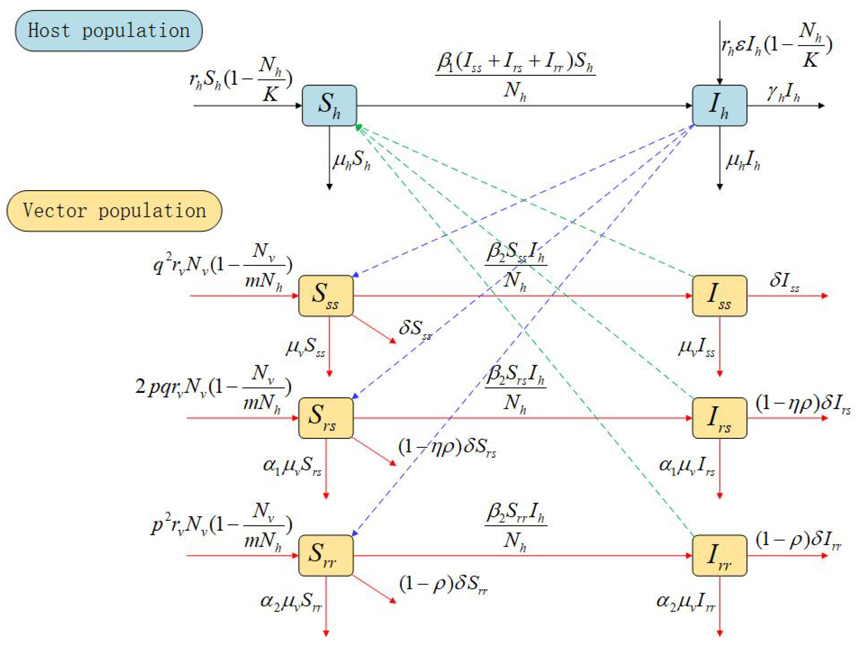
• We assume that the replanting rate is determined by the abundance or density of plants, using $r_h{S}_h(1-{\displaystyle \frac{N_h}{K}})$ and $ϵr_h{I}_h(1-{\displaystyle \frac{N_h}{K}})$ to describe the logistic growth of healthy and infected plants, respectively. In these equations, r represents the intrinsic growth rate of healthy plants, $ϵ$ ($0\le ϵ<1$) denotes the proportional reduction in the replacement rate for infected plants, and K is the maximum capacity for planting citrus trees in the orchard;
• The forces of infection for HLB transmission, namely the infection rates, are defined as follows: ${\displaystyle \frac{{\beta }_1(I_{ss}+I_{rs}+I_{rr})}{N_h}}$ represents the vector-to-host transmission rate, while ${\displaystyle \frac{{\beta }_2{I}_h}{N_h}}$ represents the host-to-vector transmission rate, where ${\beta }_1$ is the transmission probability from infectious ACP to susceptible citrus trees, and ${\beta }_2$ is the transmission probability from infectious citrus trees to susceptible ACP. Additionally, the natural mortality rate of citrus trees is given by ${\mu }_h$, and the roguing rate of infected citrus trees is represented by ${\gamma }_h$;
• It is assumed that mating among adult ACPs (between individuals of opposite sexes) occurs randomly [16]. In other words, all adult ACPs have an equal chance of reproducing and mate with any other adult ACP of the opposite sex with the same probability. The presence or absence of insecticide resistance is determined by a pair of alleles in the ACP population, which in turn affects the parameters for ACP mortality and growth rates. The insecticide-sensitive allele is denoted by S, and the insecticide-resistant allele by R. Thus, following the idea outlined in [16,19], we take the frequency of each allele using the following formulas:

  $$q\left(t\right)={\displaystyle \frac{N_{ss}^v\left(t\right)+\frac{1}{2}{N}_{rs}^v\left(t\right)}{N_v\left(t\right)}}\mathrm{and}p\left(t\right)={\displaystyle \frac{N_{rr}^v\left(t\right)+\frac{1}{2}{N}_{rs}^v\left(t\right)}{N_v\left(t\right)}},$$

  where $q\left(t\right)$ and $p\left(t\right)$ represent the frequencies of S and R alleles at time t, respectively. Therefore, the probability of forming an $SS$ genotype is given $q\left(t\right)\times q\left(t\right)=q^2\left(t\right)$. Similarly, the probability of forming an $RS$-genotype is $2p\left(t\right)\times q\left(t\right)=2p\left(t\right)q\left(t\right)$ (which accounts for $p\left(t\right)\times q\left(t\right)$ for $RS$ plus $q\left(t\right)\times p\left(t\right)$ for $SR$), while the probability of forming an $RR$-genotype is $p\left(t\right)\times p\left(t\right)=p^2\left(t\right)$. Consequently, the proportions of the $SS$, $RS$, and $RR$ genotypes in the next generation can be calculated as $q^2\left(t\right)$, $2p\left(t\right)q\left(t\right)$, and $p{\left(t\right)}^2$, respectively, [16]. It is important to note that $q\left(t\right)+p\left(t\right)=1$, and $q^2\left(t\right)+2p\left(t\right)q\left(t\right)+p^2\left(t\right)=1$ for all time $t\ge 0$ (which reflects the Hardy–Weinberg principle in population genetics [16,19]). The following Verhulst–Pearl logistic birth functions for the $SS$, $RS$, and $RR$ genotypes (denoted as $B_{ss}$, $B_{rs}$, and $B_{rr}$, respectively) are adopted:

  $$\begin{array}{c}{B}_{ss}=q^2{r}_v{N}_v\left(1-{\displaystyle \frac{N_v}{m{N}_h}}\right),B_{rs}=2pq{r}_v{N}_v\left(1-{\displaystyle \frac{N_v}{m{N}_h}}\right),B_{rr}=p^2{r}_v{N}_v\left(1-{\displaystyle \frac{N_v}{m{N}_h}}\right),\hfill \end{array}$$

  where $r_v$ is the oviposition rate of adult ACP, and m is the average carrying capacity of ACPs per citrus tree;
• Note that ACP insecticide resistance is inherited (vertically) [16,20]; that is, an insecticide-resistant adult ACP produces insecticide-resistant offspring. Susceptible ACPs of all genotypes ($S_{ss}$, $S_{rs}$, and $S_{rr}$) acquire HLB infection at a rate of ${\displaystyle \frac{{\beta }_2{I}_h}{N_h}}$. ACPs of the $SS$-genotype ($S_{ss}$ and $I_{ss}$) experience natural mortality at a rate of ${\mu }_v$, as well as additional mortality due to insecticide use at a rate of $\delta$;
• It is further assumed that there is a mortality fitness cost associated with both homozygous resistant and heterozygous ACPs [21,22,23]. Specifically, ACPs of the $RR$ genotype experience natural mortality at a rate of ${\alpha }_2{\mu }_v$ (with ${\alpha }_2\ge 1$ reflecting the increased mortality rate of $RR$ genotype ACPs due to the fitness cost, compared to the natural mortality rate of $SS$ genotype ACPs). ACPs of the $RS$ genotype suffer natural mortality at a rate of ${\alpha }_1{\mu }_v$ (where $1\le {\alpha }_1\le {\alpha }_2$ represents the increased mortality rate of $RS$ genotype ACPs due to the fitness cost, compared to $SS$ genotype ACPs). Note that ${\alpha }_1={\alpha }_2$ if the resistant allele (R) is dominant, and ${\alpha }_1=1$ if the R allele is recessive;
• The population of ACPs with the $SS$ genotype decreases due to insecticide use at a rate of $\delta$. Similarly, the population of $RR$ genotype decreases at a rate of $(1-\rho )\delta$, where $0\le \rho \le 1$ is a modification parameter that accounts for the assumed decrease in mortality rate of $RR$ genotype vectors due to insecticides, compared to $SS$ genotype vectors (due to the mortality fitness cost). Additionally, $RS$ genotype vectors experience mortality from insecticide use at a rate of $(1-\eta \rho )\delta$, where $0\le \eta \le 1$ is a modification parameter that reflects the degree of dominance of the resistant allele (i.e., $\eta =1$ models the case where the resistant allele is dominant, while $\eta =0$ represents the scenario when it is recessive). The parameter $\eta$ of the resistant allele measures the relative impact of the $RS$ heterozygote compared to the two corresponding homozygote genotypes, $SS$ and $RR$ (see [18]).

Based on the above assumptions, we establish the HLB model incorporating resistance for ACP population as a system of first-order nonlinear ordinary differential equations as follows:

$$\left\{\begin{array}{c}{\displaystyle \frac{\mathrm{d}{S}_h}{\mathrm{d}t}}=r_h{S}_h\left(1-{\displaystyle \frac{N_h}{K}}\right)-{\displaystyle \frac{{\beta }_1(I_{ss}+I_{rs}+I_{rr})S_h}{N_h}}-{\mu }_h{S}_h,\hfill \\ {\displaystyle \frac{\mathrm{d}{I}_h}{\mathrm{d}t}}=r_hϵI_h\left(1-{\displaystyle \frac{N_h}{K}}\right)+{\displaystyle \frac{{\beta }_1(I_{ss}+I_{rs}+I_{rr})S_h}{N_h}}-({\gamma }_h+{\mu }_h)I_h,\hfill \\ {\displaystyle \frac{\mathrm{d}{S}_{ss}}{\mathrm{d}t}}=q^2{r}_v{N}_v\left(1-{\displaystyle \frac{N_v}{m{N}_h}}\right)-{\displaystyle \frac{{\beta }_2{S}_{ss}{I}_h}{N_h}}-({\mu }_v+\delta )S_{ss},\hfill \\ {\displaystyle \frac{\mathrm{d}{I}_{ss}}{\mathrm{d}t}}={\displaystyle \frac{{\beta }_2{S}_{ss}{I}_h}{N_h}}-({\mu }_v+\delta )I_{ss},\hfill \\ {\displaystyle \frac{\mathrm{d}{S}_{rs}}{\mathrm{d}t}}=2pq{r}_v{N}_v\left(1-{\displaystyle \frac{N_v}{m{N}_h}}\right)-{\displaystyle \frac{{\beta }_2{S}_{rs}{I}_h}{N_h}}-({\alpha }_1{\mu }_v+(1-\eta \rho )\delta )S_{rs},\hfill \\ {\displaystyle \frac{\mathrm{d}{I}_{rs}}{\mathrm{d}t}}={\displaystyle \frac{{\beta }_2{S}_{rs}{I}_h}{N_h}}-({\alpha }_1{\mu }_v+(1-\eta \rho )\delta )I_{rs},\hfill \\ {\displaystyle \frac{\mathrm{d}{S}_{rr}}{\mathrm{d}t}}=p^2{r}_v{N}_v\left(1-{\displaystyle \frac{N_v}{m{N}_h}}\right)-{\displaystyle \frac{{\beta }_2{S}_{rr}{I}_h}{N_h}}-({\alpha }_2{\mu }_v+(1-\rho )\delta )S_{rr},\hfill \\ {\displaystyle \frac{\mathrm{d}{I}_{rr}}{\mathrm{d}t}}={\displaystyle \frac{{\beta }_2{S}_{rr}{I}_h}{N_h}}-({\alpha }_2{\mu }_v+(1-\rho )\delta )I_{rr}.\hfill \end{array}\right.$$

(1)

A schematic diagram of the model is depicted in Figure 1, and the state variables and the parameters are described in

Table 1. Description of the variables and parameters for the HLB model (1).

Variable	Description
$S_h$	Population of susceptible citrus trees
$I_h$	Population of infected citrus trees
$S_{ss}$	Population of susceptible sensitive ACP
$I_{ss}$	Population of infected sensitive ACP
$S_{rs}$	Population of susceptible resistant ACP
$I_{rs}$	Population of infected sensitive ACP
$S_{rr}$	Population of susceptible sensitive ACP
$I_{rr}$	Population of infected resistant ACP
Parameter	Description
K	Environmental carrying capacity of citrus trees
$r_h$	Recruitment rate of citrus trees
${\beta }_1$	Transmission probability from infected ACP to susceptible citrus trees
${\mu }_h$	Natural mortality rate in citrus trees
$ϵ$	Probability that a diseased citrus trees sapling is not removed
${\gamma }_h$	The roguing rate of infected citrus trees
$r_v$	Recruitment rate of ACP
m	Average carrying capacity of ACP per citrus tree
${\beta }_2$	Transmission probability from infected citrus trees to susceptible ACP
${\mu }_v$	Natural mortality rate of ACP
$\delta$	Death rate due to the (encounter with) insecticides for $SS$ genotype ACP
${\alpha }_1$	Modification parameter in natural mortality rate of $RS$ genotype ACP due to fitness cost in comparison to the natural mortality rate of $SS$ genotype ACP
${\alpha }_2$	Modification parameter in natural mortality rate of $RR$ genotype ACP due to fitness cost in comparison to the natural mortality rate of $SS$ genotype ACP
$\rho$	Modification parameter in death rate of $RR$ genotype ACP due to the insecticides in comparison to the death rate of $SS$ genotype ACP
$\eta$	Modification parameter in death rate of $RS$ genotype ACP due to the insecticides in comparison to the death rate of $RR$ genotype ACP

.

The basic qualitative properties of the model (1) will be explored in the subsequent section.

3. Model Analysis

3.1. Basic Properties

To better organize the analysis, we simplify certain terms in the model by defining $d_1={\gamma }_h+{\mu }_h,$ $d_2={\mu }_v+\delta ,$ $d_3={\alpha }_1{\mu }_v+(1-\eta \rho )\delta ,$ $d_4={\alpha }_2{\mu }_v+(1-\rho )\delta$. Consequently, the model (1) can be rewritten as follows:

$$\left\{\begin{array}{c}{\displaystyle \frac{\mathrm{d}{S}_h}{\mathrm{d}t}}=r_h{S}_h\left(1-{\displaystyle \frac{N_h}{K}}\right)-{\displaystyle \frac{{\beta }_1(I_{ss}+I_{rs}+I_{rr})S_h}{N_h}}-{\mu }_h{S}_h,\hfill \\ {\displaystyle \frac{\mathrm{d}{I}_h}{\mathrm{d}t}}=r_hϵI_h\left(1-{\displaystyle \frac{N_h}{K}}\right)+{\displaystyle \frac{{\beta }_1(I_{ss}+I_{rs}+I_{rr})S_h}{N_h}}-d_1{I}_h,\hfill \\ {\displaystyle \frac{\mathrm{d}{S}_{ss}}{\mathrm{d}t}}=q^2{r}_v{N}_v\left(1-{\displaystyle \frac{N_v}{m{N}_h}}\right)-{\displaystyle \frac{{\beta }_2{S}_{ss}{I}_h}{N_h}}-d_2{S}_{ss},\hfill \\ {\displaystyle \frac{\mathrm{d}{I}_{ss}}{\mathrm{d}t}}={\displaystyle \frac{{\beta }_2{S}_{ss}{I}_h}{N_h}}-d_2{I}_{ss},\hfill \\ {\displaystyle \frac{\mathrm{d}{S}_{rs}}{\mathrm{d}t}}=2pq{r}_v{N}_v\left(1-{\displaystyle \frac{N_v}{m{N}_h}}\right)-{\displaystyle \frac{{\beta }_2{S}_{rs}{I}_h}{N_h}}-d_3{S}_{rs},\hfill \\ {\displaystyle \frac{\mathrm{d}{I}_{rs}}{\mathrm{d}t}}={\displaystyle \frac{{\beta }_2{S}_{rs}{I}_h}{N_h}}-d_3{I}_{rs},\hfill \\ {\displaystyle \frac{\mathrm{d}{S}_{rr}}{\mathrm{d}t}}=p^2{r}_v{N}_v\left(1-{\displaystyle \frac{N_v}{m{N}_h}}\right)-{\displaystyle \frac{{\beta }_2{S}_{rr}{I}_h}{N_h}}-d_4{S}_{rr},\hfill \\ {\displaystyle \frac{\mathrm{d}{I}_{rr}}{\mathrm{d}t}}={\displaystyle \frac{{\beta }_2{S}_{rr}{I}_h}{N_h}}-d_4{I}_{rr},\hfill \end{array}\right.$$

(2)

Define $f_1=\min \{d_2,d_3,d_4\}$ and $f_2=\max \{d_2,d_3,d_4\}$. Let

$$\begin{array}{c}{G}_h=\left\{(S_h\left(t\right),I_h\left(t\right))\in R_{+}^2:0<N_h\left(t\right)\le N_h^0\right\},\hfill \end{array}$$

$$\begin{array}{c}{G}_v=\{(S_{ss}\left(t\right),I_{ss}\left(t\right),S_{rs}\left(t\right),I_{rs}\left(t\right),S_{rr}\left(t\right),I_{rr}\left(t\right))\in R_{+}^6:0<N_v\left(t\right)\le N_v^0\},\hfill \end{array}$$

where $N_h^0=(1-{\displaystyle \frac{{\mu }_h}{r_h}})K$, $N_v^0=(1-{\displaystyle \frac{f_1}{r_v}})m{N}_h^0$.

All state variables in model (2) are non-negative, as they represent populations of citrus trees and ACPs.

Lemma 1.

Denote $\Gamma \left(t\right)={(S_h\left(t\right),I_h\left(t\right),S_{ss}\left(t\right),I_{ss}\left(t\right),S_{rs}\left(t\right),I_{rs}\left(t\right),S_{rr}\left(t\right),I_{rr}\left(t\right))}^T$. Assume the initial condition $\Gamma \left(0\right)\gg 0$. Then, the solutions $\Gamma \left(t\right)$ of model (2) remain non-negative for all $t>0$. Furthermore,

$$0<\underset{t\to \infty }{\mathrm{lim\; inf}} N_h\left(t\right)\le \underset{t\to \infty }{\mathrm{lim\; sup}} N_h\left(t\right)\le N_h^0,0<\underset{t\to \infty }{\mathrm{lim\; inf}} N_v\left(t\right)\le \underset{t\to \infty }{\mathrm{lim\; sup}} N_v\left(t\right)\le N_v^0.$$

The region $G=G_h\times G_v\subset R_{+}^8$ is positively invariant for model (2) with non-negative initial conditions.

Proof of Lemma 1.

Assume the initial data of model (2) are $\Gamma \left(0\right)\gg 0$. Suppose that the solution components of the model equation are not positive, then there exists a first time $\overline{t}>0$ defined as follows:

$$\overline{t}=\inf \left\{t|S_h\left(t\right)=0\mathrm{or}{I}_h\left(t\right)=0\mathrm{or}{S}_{ss}\left(t\right)=0\mathrm{or}{I}_{ss}\left(t\right)=0\mathrm{or}{S}_{rs}\left(t\right)=0\mathrm{or}{S}_{rr}\left(t\right)=0\mathrm{or}{I}_{rr}\left(t\right)=0\right\}.$$

Now if $I_h\left(\overline{t}\right)=0$, $S_h\left(t\right)>0,$ $S_{ss}\left(t\right)>0,$ $I_{ss}\left(t\right)>0,$ $S_{rs}\left(t\right)>0,$ $I_{rs}\left(t\right)>0,$ $S_{rr}\left(t\right)>0,$ $I_{rr}\left(t\right)>0,$ for $t\in (0,\overline{t})$, then ${\displaystyle \frac{d{I}_h\left(\overline{t}\right)}{dt}}<0.$ It follows from the second equation of model (2) that

$${\displaystyle \frac{d{I}_h\left(\overline{t}\right)}{dt}}={\displaystyle \frac{{\beta }_1(I_{ss}+I_{rs}+I_{rr})S_h}{N_h}}>0.$$

This is a contradiction. Thus, $I_h\left(t\right)>0$ for all $t>0$. In a similar manner, we can establish that all the solutions $S_{ss}\left(t\right), I_{ss}\left(t\right), S_{rs}\left(t\right), I_{rs}\left(t\right), S_{rr}\left(t\right), I_{rr}\left(t\right)$ are positive for all $t>0$.

Additionally, it is evident that

$${\displaystyle \frac{\mathrm{d}{S}_h}{\mathrm{d}t}}=\left(r_h(1-{\displaystyle \frac{N_h}{K}})-{\displaystyle \frac{{\beta }_1(I_{ss}+I_{rs}+I_{rr})}{N_h}}-{\mu }_h\right)S_h.$$

Thus,

$$S_h(t)=S_h(0)e^{{\int }_0^t(r_h(1-{\displaystyle \frac{N_h}{K}})-{\displaystyle \frac{{\beta }_1(I_{ss}+I_{rs}+I_{rr})}{N_h}}-{\mu }_h)ds}>0,\mathrm{for}\mathrm{all}t>0.$$

Adding the first and second equations of model (2), the total number of citrus trees $N_h\left(t\right)$ satisfies

$${\displaystyle \frac{\mathrm{d}{N}_h}{\mathrm{d}t}}=r_h{S}_h\left(1-{\displaystyle \frac{N_h}{K}}\right)+r_hϵI_h\left(1-{\displaystyle \frac{N_h}{K}}\right)-{\mu }_h{S}_h-d_1{I}_h\le r_h{N}_h\left(1-{\displaystyle \frac{N_h}{K}}\right)-{\mu }_h{N}_h,$$

This implies that

$${\displaystyle \underset{t\to \infty }{\mathrm{lim\; sup}} N_h\left(t\right)\le \left(1-\frac{{\mu }_h}{r_h}\right)K=N_h^0.}$$

(3)

Adding the third to eighth equations of model (2), the total number of ACP $N_v\left(t\right)$ satisfies

$$\begin{array}{cc}{\displaystyle \frac{\mathrm{d}{N}_v}{\mathrm{d}t}}\hfill & =r_v{N}_v\left(1-{\displaystyle \frac{N_v}{m{N}_h}}\right)-d_2{S}_{ss}-d_2{I}_{ss}-d_3{S}_{rs}-d_3{I}_{rs}-d_4{S}_{rr}-d_4{I}_{rr}\hfill \\ \hfill & \le r_v{N}_v\left(1-{\displaystyle \frac{N_v}{m{N}_h^0}}\right)-f_1{N}_v.\hfill \end{array}$$

Thus,

$${\displaystyle \underset{t\to \infty }{\mathrm{lim\; sup}} N_v\left(t\right)\le \left(1-\frac{f_1}{r_v}\right)m{N}_h^0=N_v^0.}$$

(4)

It follows from (3) and (4) that the region G is positively invariant. □

It should be noted that the upper bound of $N_h\left(t\right)$, given by $N_h^0=(1-{\displaystyle \frac{{\mu }_h}{r_h}})K$, is positive if $r_h>{\mu }_h$. This implies that the growth rate of the citrus trees ($r_h$) must exceed the natural death rate (${\mu }_h$) for the population to be sustainable. In a closed environment, without immigration or migration, if the death rate of citrus trees exceeds the birth rate, the citrus tree population will eventually die out. Thus, if $r_h<{\mu }_h$, the citrus tree population will eventually decline to zero. Similarly, the upper bound of $N_v\left(t\right)$, given by $N_v^0=(1-{\displaystyle \frac{f_1}{r_v}})m{N}_h^0$, is positive if $r_v>f_1$. This means that the ACP growth rate ($r_v$) must be greater than the minimum mortality rate of the three psyllid classes ($f_1$), which includes effects from both natural causes and insecticides. In a closed environment, without immigration or migration, if the minimum mortality rate exceeds the birth rate, the ACP population will eventually die out. Therefore, if $r_v<f_1$, the ACP population will eventually decline to zero (i.e., the disease will die out if $r_v<f_1$). For the remainder of this study, it is assumed that $r_h>{\mu }_h$ and $r_v>f_1$, ensuring that both citrus trees and ACP populations persist in the study area.

3.2. Existence of Disease-Free Equilibria

The disease-free equilibrium (DFE) of the model (2) is obtained by setting all infected components $(I_h,I_{ss},I_{rs},I_{rr})$ to zero. The non-infected components at the DFE, denoted by $(S_h^{*},S_{ss}^{*},S_{rs}^{*},S_{rr}^{*})$, are given by $q^{*}={\displaystyle \frac{S_{ss}^{*}+\frac{1}{2}{S}_{rs}^{*}}{N_v^{*}}},$ and $p^{*}={\displaystyle \frac{S_{rr}^{*}+\frac{1}{2}{S}_{rs}^{*}}{N_v^{*}}},$ where $N_v^{*}=S_{ss}^{*}+S_{rs}^{*}+S_{rr}^{*}.$ It can be shown at the DFE that $q^{*}$ satisfies the following equation:

$$\begin{array}{c}{q}^{*}(q^{*}-1)[g_1{q}^{*}-d_2(d_3-d_4)]=0,\hfill \end{array}$$

(5)

where $g_1=d_2(d_3-d_4)+d_4(d_3-d_2)$.

Lemma 2.

It follows from Equation (5) that at the disease-free equilibrium (DFE), $q^{*}$ and $p^{*}$ can take values from any one of the following four cases (this follows from the solution of Equation (5)) assuming a positive initial ACP population:

(i) 

$q^{*}=1$ and $p^{*}=0$;

(ii) 

$q^{*}=0$ and $p*=1$;

(iii) 

$q^{*}={\displaystyle \frac{d_2(d_3-d_4)}{g_1}}$ and $p^{*}={\displaystyle \frac{d_4(d_3-d_2)}{g_1}}$, provided that $(d_3-d_2)(d_3-d_4)>0$;

(iv) 

any value $q^{*},$ $p^{*}$ in $[0,1]$ with $p^{*}+q^{*}=1$, provided that $d_2=d_3=d_4.$

It should be noted that $q^{*}$ and $p^{*}$ under the assumption stated in Lemma 2 must satisfy the equality $p^{*}+q^{*}=1$ in all cases. Therefore, the model (2) has five disease-free equilibria as given below:

(S1) The trivial equilibrium (TE), denoted by $E_{00}$,

$$\begin{array}{cc}{E}_{00}\hfill & =\left({\left(S_h^{*}\right)}^0,{\left(I_h^{*}\right)}^0,{\left(S_{ss}^{*}\right)}^0,{\left(I_{ss}^{*}\right)}^0,{\left(S_{rs}^{*}\right)}^0,{\left(I_{rs}^{*}\right)}^0,{\left(S_{rr}^{*}\right)}^0,{\left(I_{rr}^{*}\right)}^0\right)\hfill \\ \hfill & =\left(0,0,0,0,0,0,0,0\right).\hfill \end{array}$$

(S2) The trivial disease-free equilibrium (TDFE), denoted by $E_{0T}$,

$$\begin{array}{cc}{E}_{0T}\hfill & =\left({\left(S_h^{*}\right)}^T,{\left(I_h^{*}\right)}^T,{\left(S_{ss}^{*}\right)}^T,{\left(I_{ss}^{*}\right)}^T,{\left(S_{rs}^{*}\right)}^T,{\left(I_{rs}^{*}\right)}^T,{\left(S_{rr}^{*}\right)}^T,{\left(I_{rr}^{*}\right)}^T\right)\hfill \\ \hfill & =\left(N_h^0,0,0,0,0,0,0,0\right).\hfill \end{array}$$

(S3) The non-trivial sensitive-only disease-free boundary equilibrium (NTSDFE), denoted by $E_{0S}$, occurring when $q^{*}=1$ and $p^{*}=0$,

$$\begin{array}{cc}{E}_{0S}\hfill & =\left({\left(S_h^{*}\right)}^S,{\left(I_h^{*}\right)}^S,{\left(S_{ss}^{*}\right)}^S,{\left(I_{ss}^{*}\right)}^S,{\left(S_{rs}^{*}\right)}^S,{\left(I_{rs}^{*}\right)}^S,{\left(S_{rr}^{*}\right)}^S,{\left(I_{rr}^{*}\right)}^S\right)\hfill \\ \hfill & =\left(N_h^0,0,N_{ss}^{*},0,0,0,0,0\right),\hfill \end{array}$$

where $N_{ss}^{*}={\displaystyle \frac{(r_v-d_2)}{r_v}}m{N}_h^0$.

(S4) The non-trivial resistant-only disease-free boundary equilibrium (NTRDFE), denoted by $E_{0R}$, occurring when $q^{*}=0$ and $p^{*}=1$,

$$\begin{array}{cc}{E}_{0R}\hfill & =\left({\left(S_h^{*}\right)}^R,{\left(I_h^{*}\right)}^R,{\left(S_{ss}^{*}\right)}^R,{\left(I_{ss}^{*}\right)}^R,{\left(S_{rs}^{*}\right)}^R,{\left(I_{rs}^{*}\right)}^R,{\left(S_{rr}^{*}\right)}^R,{\left(I_{rr}^{*}\right)}^R\right)\hfill \\ \hfill & =\left(N_h^0,0,0,0,0,0,N_{rr}^{*},0\right),\hfill \end{array}$$

where $N_{rr}^{*}={\displaystyle \frac{(r_v-d_4)}{r_v}}m{N}_h^0$.

(S5) The non-trivial co-existence disease-free equilibrium (NTCDFE), denoted by $E_{0C}$, occurring when $q^{*}>0$ and $p^{*}>0$,

$$\begin{array}{cc}{E}_{0C}\hfill & =\left({\left(S_h^{*}\right)}^C,{\left(I_h^{*}\right)}^C,{\left(S_{ss}^{*}\right)}^C,{\left(I_{ss}^{*}\right)}^C,{\left(S_{rs}^{*}\right)}^C,{\left(I_{rs}^{*}\right)}^C,{\left(S_{rr}^{*}\right)}^C,{\left(I_{rr}^{*}\right)}^C\right)\hfill \\ \hfill & =\left(N_h^0,0,S_{ss}^{*},0,S_{rs}^{*},0,S_{rr}^{*},0\right)\hfill \end{array}$$

where

$$S_{ss}^{*}={\displaystyle \frac{{\left(q^{*}\right)}^2{r}_v(g_2-1)}{d_2{g}_2^2}}m{N}_h^0,S_{rs}^{*}={\displaystyle \frac{2p^{*}{q}^{*}{r}_v(g_2-1)}{d_3{g}_2^2}}m{N}_h^0,S_{rr}^{*}={\displaystyle \frac{{\left(p^{*}\right)}^2{r}_v(g_2-1)}{d_4{g}_2^2}}m{N}_h^0,$$

(6)

with, $q^{*}$ and $p^{*}$ are determined by either option (iii) or (iv) of the possible solutions presented in Lemma 2 and $g_2={\displaystyle \frac{{\left(q^{*}\right)}^2{r}_v}{d_2}}+{\displaystyle \frac{2p^{*}{q}^{*}{r}_v}{d_3}}+{\displaystyle \frac{{\left(p^{*}\right)}^2{r}_v}{d_4}}$.

From Equation (6), we have

(1)

The NTSDFE ($E_{0S}$) exists if and only if $r_v>d_2$;

(2)

The NTRDFE ($E_{0R}$) exists if and only if $r_v>d_4$;

(3)

The NTCDFE ($E_{0C}$) exists if and only if $g_2>1$ and $(d_3-d_2)(d_3-d_4)>0$, or if and only if $g_2>1$ and $d_2=d_3=d_4.$

It is easy to prove that the trivial equilibrium $E_{00}$ is always unstable. The local asymptotic stability of the TDFE ($E_{0T}$), the NTSDFE ($E_{0S}$), NTRDFE ($E_{0R}$), and NTCDFE ($E_{0C}$) will be discussed in the following subsection.

For convenience, we define the following general nontrivial disease-free equilibrium of the model (2), denoted by $E_{0f}$:

$$\begin{array}{cc}{E}_{0f}\hfill & =\left({\left(S_h^{*}\right)}^f,{\left(I_h^{*}\right)}^f,{\left(S_{ss}^{*}\right)}^f,{\left(I_{ss}^{*}\right)}^f,{\left(S_{rs}^{*}\right)}^f,{\left(I_{rs}^{*}\right)}^f,{\left(S_{rr}^{*}\right)}^f,{\left(I_{rr}^{*}\right)}^f\right)\hfill \\ \hfill & =\left(N_h^0,0,S_{ss}^0,0,S_{rs}^0,0,S_{rr}^0,0\right).\hfill \end{array}$$

(7)

That is,

(i)

If $E_{0f}=E_{0T}$, then $S_{ss}^0=0$, $S_{rs}^0=0$ and $S_{rr}^0=0$;

(ii)

If $E_{0f}=E_{0S}$, then $S_{ss}^0=N_{ss}^{*}$, $S_{rs}^0=0$ and $S_{rr}^0=0$;

(iii)

If $E_{0f}=E_{0R}$, then $S_{ss}^0=0$, $S_{rs}^0=0$ and $S_{rr}^0=N_{rr}^{*}$;

(iv)

If $E_{0f}=E_{0C}$, then $S_{ss}^0=S_{ss}^{*}$, $S_{rs}^0=S_{rs}^{*}$ and $S_{rr}^0=S_{rr}^{*}$.

For the group of infected individuals, we can observe that $I_h^{*}=0$ if and only if $I_{ss}^{*}=0$, $I_{rs}^{*}=0$ and $I_{rr}^{*}=0$. Therefore, The system (2) has no other boundary equilibrium points apart from the five disease-free equilibrium points. In addition, due to the high dimensionality of the system (2), the existence and stability of the endemic equilibrium point are difficult to discuss. This paper will not address those issues.

3.3. Local Asymptotic Stability of Equilibria

The local stability of $E_{0f}$ is determined by the basic reproduction number $R_{0f}$, which can be calculated from the next-generation matrix for the system (2). The model includes four infection groups: $I_h,I_{ss},I_{rs}$, and $I_{rr}$. Using the notation of van den Driessche and Watmough [24], the new infection terms and the remaining transfer terms for these four groups are presented below in partitioned form.

Denote

$$\mathcal{F}=\left(\begin{array}{c}{r}_hϵ\left(1-{\displaystyle \frac{N_h}{K}}\right)I_h+{\displaystyle \frac{{\beta }_1\left(I_{ss}+I_{rs}+I_{rr}\right)S_h}{N_h}}\\ {\displaystyle \frac{{\beta }_2{S}_{ss}{I}_h}{N_h}}\\ {\displaystyle \frac{{\beta }_2{S}_{rs}{I}_h}{N_h}}\\ {\displaystyle \frac{{\beta }_2{S}_{rr}{I}_h}{N_h}}\end{array}\right),\mathcal{V}=\left(\begin{array}{c}{d}_1{I}_h\\ d_2{I}_{ss}\\ d_3{I}_{rs}\\ d_4{I}_{rr}\end{array}\right).$$

Thus, at point $E_0$, the Jacobian matrices of $\mathcal{F}$ and $\mathcal{V}$ with respect to the four groups yield

$$F=\left(\begin{array}{cccc}ϵr_h\left(1-{\displaystyle \frac{N_h^0}{K}}\right)& {\beta }_1& {\beta }_1& {\beta }_1\\ {\displaystyle \frac{{\beta }_2{S}_{ss}^0}{N_h^0}}& 0& 0& 0\\ {\displaystyle \frac{{\beta }_2{S}_{rs}^0}{N_h^0}}& 0& 0& 0\\ {\displaystyle \frac{{\beta }_2{S}_{rr}^0}{N_h^0}}& 0& 0& 0\end{array}\right),V=\left(\begin{array}{ccccc}{d}_1& 0& 0& 0& \\ 0& d_2& 0& 0\\ 0& 0& d_3& 0\\ 0& 0& 0& d_4\end{array}\right),$$

(8)

where F is a non-negative matrix and V is a non-singular matrix. The basic reproduction number $R_{0f}$ is given by $\rho \left(F{V}^{-1}\right)$, which is the spectral radius of the matrix $F{V}^{-1}$.

Denote

$$R_1={\displaystyle \frac{ϵr_h\left(K-N_h^0\right)}{K{d}_1}}={\displaystyle \frac{ϵ{\mu }_h}{d_1}},R_2={\displaystyle \frac{{\beta }_1{\beta }_2}{d_1{N}_h^0}}\left({\displaystyle \frac{S_{ss}^0}{d_2}}+{\displaystyle \frac{S_{rs}^0}{d_3}}+{\displaystyle \frac{S_{rr}^0}{d_4}}\right).$$

The basic reproduction number of model (2), denoted as $R_0$, is

$$R_0={\displaystyle \frac{1}{2}}\left(R_1+\sqrt{R_1^2+4R_2}\right).$$

(9)

It is convenient to define the following threshold quantities:

$$R_0^{0t}=R_0{|}_{E_{0f}=E_{0T}}={\displaystyle \frac{ϵ{\mu }_h}{d_1}},$$

(10)

$$R_0^{0s}=R_0{|}_{E_{0f}=E_{0S}}={\displaystyle \frac{1}{2}}\left({\displaystyle \frac{ϵ{\mu }_h}{d_1}}+\sqrt{{\left({\displaystyle \frac{ϵ{\mu }_h}{d_1}}\right)}^2+{\displaystyle \frac{4{\beta }_1{\beta }_2{N}_{ss}^{*}}{d_1{d}_2{N}_h^0}}}\right),$$

(11)

$$R_0^{0r}=R_0{|}_{E_{0f}=E_{0R}}={\displaystyle \frac{1}{2}}\left({\displaystyle \frac{ϵ{\mu }_h}{d_1}}+\sqrt{{\left({\displaystyle \frac{ϵ{\mu }_h}{d_1}}\right)}^2+{\displaystyle \frac{4{\beta }_1{\beta }_2{N}_{rr}^{*}}{d_1{d}_4{N}_h^0}}}\right),$$

(12)

$$R_0^{0c}=R_0{|}_{E_{0f}=E_{0C}}={\displaystyle \frac{1}{2}}\left({\displaystyle \frac{ϵ{\mu }_h}{d_1}}+\sqrt{{\left({\displaystyle \frac{ϵ{\mu }_h}{d_1}}\right)}^2+{\displaystyle \frac{4{\beta }_1{\beta }_2}{d_1{N}_h^0}}\left({\displaystyle \frac{S_{ss}^{*}}{d_2}}+{\displaystyle \frac{S_{rs}^{*}}{d_3}}+{\displaystyle \frac{S_{rr}^{*}}{d_4}}\right)}\right).$$

(13)

Therefore, based on the above analysis and Theorem 2 in [24], the following result is established.

Theorem 1.

For model (2), the following results hold.

(a) 

When $(d_3-d_2)(d_3-d_4)>0$ or $d_2=d_3=d_4$ and $g_2>1$, the NTCDFE $E_{0C}$ is locally asymptotically stable if $R_0^{0c}<1$ and unstable if $R_0^{0c}>1$.

(b) 

When $r_v>d_2$, the NTSDFE $E_{0S}$ is locally asymptotically stable if $R_0^{0s}<1$ and unstable if $R_0^{0s}>1$;

(c) 

When $r_v>d_4$, the NTRDFE $E_{0R}$ is locally asymptotically stable if $R_0^{0r}<1$ and unstable if $R_0^{0r}>1$;

(d) 

The TDFE $E_{0T}$ is always locally asymptotically stable.

It is noted that from Theorem 1, if the equilibrium point $E_{0X}$ ($X=C,S,R$) exists, then it must be locally stable provided that $R_0^{0x}<1$ ($x=c,s,r$).

3.4. Global Asymptotic Stability of Equilibria

In this section, we will explore the global asymptotic stability of the nontrivial disease-free equilibrium $E_{0f}$ for the special case of model (2), where disease-induced mortality in citrus trees is negligible (i.e., ${\gamma }_h=0$) and diseased citrus tree saplings are not removed (i.e., $ϵ=1$). These assumptions are made to simplify the mathematical analysis.

By adding the first and second equations of model (2), and noting that ${\gamma }_h=0$ and $ϵ=1$, we obtain

$${\displaystyle \frac{\mathrm{d}{N}_h}{\mathrm{d}t}}=r_h{N}_h\left(1-{\displaystyle \frac{N_h}{K}}\right)-{\mu }_h{N}_h={\displaystyle \frac{r_h{N}_h}{K}}(N_h^0-N_h).$$

(14)

It is clear that $N_h\left(t\right)\to N_h^0$, as $t\to \infty$. Therefore, from now on, we will use the limiting system with $N_h=N_h^0$. The equations for the infected components of model (2) can then be written as:

$$\left\{\begin{array}{c}{\displaystyle \frac{\mathrm{d}{S}_h}{\mathrm{d}t}}=r_h{S}_h\left(1-{\displaystyle \frac{N_h^0}{K}}\right)-{\displaystyle \frac{{\beta }_1(I_{ss}+I_{rs}+I_{rr})S_h}{N_h^0}}-{\mu }_h{S}_h,\hfill \\ {\displaystyle \frac{\mathrm{d}{I}_h}{\mathrm{d}t}}=r_h{I}_h\left(1-{\displaystyle \frac{N_h^0}{K}}\right)+{\displaystyle \frac{{\beta }_1(I_{ss}+I_{rs}+I_{rr})S_h}{N_h^0}}-{\mu }_h{I}_h,\hfill \\ {\displaystyle \frac{\mathrm{d}{S}_{ss}}{\mathrm{d}t}}=q^2{r}_v{N}_v(1-{\displaystyle \frac{N_v}{m{N}_h^0}})-{\displaystyle \frac{{\beta }_2{S}_{ss}{I}_h}{N_h^0}}-d_2{S}_{ss},\hfill \\ {\displaystyle \frac{\mathrm{d}{I}_{ss}}{\mathrm{d}t}}={\displaystyle \frac{{\beta }_2{S}_{ss}{I}_h}{N_h^0}}-d_2{I}_{ss},\hfill \\ {\displaystyle \frac{\mathrm{d}{S}_{rs}}{\mathrm{d}t}}=2pq{r}_v{N}_v\left(1-{\displaystyle \frac{N_v}{m{N}_h^0}}\right)-{\displaystyle \frac{{\beta }_2{S}_{rs}{I}_h}{N_h^0}}-d_3{S}_{rs},\hfill \\ {\displaystyle \frac{\mathrm{d}{I}_{rs}}{\mathrm{d}t}}={\displaystyle \frac{{\beta }_2{S}_{rs}{I}_h}{N_h^0}}-d_3{I}_{rs},\hfill \\ {\displaystyle \frac{\mathrm{d}{S}_{rr}}{\mathrm{d}t}}=p^2{r}_v{N}_v\left(1-{\displaystyle \frac{N_v}{m{N}_h^0}}\right)-{\displaystyle \frac{{\beta }_2{S}_{rr}{I}_h}{N_h^0}}-d_4{S}_{rr},\hfill \\ {\displaystyle \frac{\mathrm{d}{I}_{rr}}{\mathrm{d}t}}={\displaystyle \frac{{\beta }_2{S}_{rr}{I}_h}{N_h^0}}-d_4{I}_{rr}.\hfill \end{array}\right.$$

(15)

Additionally, define the following sets:

$$\begin{array}{cc}{G}_c=\hfill & \left\{(S_h\left(t\right),I_h\left(t\right),S_{ss}\left(t\right),I_{ss}\left(t\right),S_{rs}\left(t\right),I_{rs}\left(t\right),S_{rr}\left(t\right),I_{rr}\left(t\right))\in G:\right.\hfill \\ \hfill & \left.0<N_h\left(t\right)\le N_h^0,S_{ss}\left(t\right)\le S_{ss}^{*},S_{rs}\left(t\right)\le S_{rs}^{*},S_{rr}\left(t\right)\le S_{rr}^{*}\right\},\hfill \end{array}$$

(16)

$$\begin{array}{cc}{G}_s=\hfill & \left\{(S_h\left(t\right),I_h\left(t\right),S_{ss}\left(t\right),I_{ss}\left(t\right),S_{rs}\left(t\right),I_{rs}\left(t\right),S_{rr}\left(t\right),I_{rr}\left(t\right))\in G\right.\hfill \\ \hfill & \left.0<N_h\left(t\right)\le N_h^0,S_{ss}\left(t\right)\le N_{ss}^{*},S_{rs}\left(t\right)=0,S_{rr}\left(t\right)=0\right\},\hfill \end{array}$$

(17)

$$\begin{array}{cc}{G}_r=\hfill & \{(S_h\left(t\right),I_h\left(t\right),S_{ss}\left(t\right),I_{ss}\left(t\right),S_{rs}\left(t\right),I_{rs}\left(t\right),S_{rr}\left(t\right),I_{rr}\left(t\right))\in G:\hfill \\ \hfill & 0<N_h\left(t\right)\le N_h^0,S_{ss}\left(t\right)=0,S_{rs}\left(t\right)=0,S_{rr}\left(t\right)\le N_{rr}^{*}\}.\hfill \end{array}$$

(18)

Lemma 3.

For model (15), the following results hold.

(a) 

If $(d_3-d_2)(d_3-d_4)>0$ or $d_2=d_3=d_4$, then the set $G_c$ is positively invariant provided that $g_2>1$ and $\min \{{\displaystyle \frac{{\left(q^{*}\right)}^2(g_2-1)}{g_2^2}},{\displaystyle \frac{2p^{*}{q}^{*}(g_2-1)}{g_2^2}},{\displaystyle \frac{{\left(p^{*}\right)}^2(g_2-1)}{g_2^2}}\}>{\displaystyle \frac{1}{4}}$.

(b) 

If $r_v>d_2$ and ${\displaystyle \frac{r_v-d_2}{r_v}}>{\displaystyle \frac{1}{4}}$, then the set $G_s$ is positively invariant.

(c) 

If $r_v>d_4$ and ${\displaystyle \frac{r_v-d_4}{r_v}}>{\displaystyle \frac{1}{4}}$, then the set $G_r$ is positively invariant.

Proof. 

First, we proof the first case. Solving Equation (14), we have

$${\displaystyle N_h\left(t\right)=\frac{N_h\left(0\right)}{(N_h^0-N_h\left(0\right))\exp (-\frac{r_h{N}_h^{0}t}{K})+N_h\left(0\right)}{N}_h^0.}$$

Consequently, if $N_h\left(0\right)\le N_h^0$, then $N_h\left(t\right)\le N_h^0$ for all $t\ge 0$. Further, it follows from the third equation of model (15) that

$$\begin{array}{cc}{\displaystyle \frac{\mathrm{d}{S}_{ss}}{\mathrm{d}t}}\hfill & =q^2{r}_v{N}_v\left(1-{\displaystyle \frac{N_v}{m{N}_h^0}}\right)-{\displaystyle \frac{{\beta }_2{S}_{ss}{I}_h}{N_h^0}}-d_2{S}_{ss},\hfill \\ \hfill & \le r_v{N}_v\left(1-{\displaystyle \frac{N_v}{m{N}_h^0}}\right)-d_2{S}_{ss},\hfill \\ \hfill & \le r_v{\displaystyle \frac{m{N}_h^0}{4}}-d_2{S}_{ss},\hfill \\ \hfill & \le r_v{\displaystyle \frac{(q^{*2}(g_2-1)}{g_2^2}}m{N}_h^0-d_2{S}_{ss},\hfill \\ \hfill & =d_2\left({\displaystyle \frac{q^{*2}{r}_v(g_2-1)}{d_2{g}_2^2}}m{N}_h^0-S_{ss}\right),\hfill \\ \hfill & =d_2(S_{ss}^{*}-S_{ss}),\hfill \end{array}$$

Hence, ${\displaystyle S_{ss}\left(t\right)=S_{ss}^{*}-(S_{ss}^{*}-S_{ss}\left(0\right))\exp -d_{2}t.}$ Therefore, if $S_{ss}\left(0\right)\le S_{ss}^{*}$, then $S_{ss}\left(t\right)\le S_{ss}^{*}$ for all $t\ge 0$. Using similar arguments, it can be shown that $S_{rs}\left(t\right)\le S_{rs}^{*}$ and $S_{rr}\left(t\right)\le S_{rr}^{*}$ for all $t\ge 0$ if if the initial conditions are within $G_c$. Thus, the set $G_c$ is positively invariant for the special case of the model (15) with $g_2\ge 1$, $\min \left\{{\displaystyle \frac{{\left(q^{*}\right)}^2(g_2-1)}{g_2^2}},{\displaystyle \frac{2p^{*}{q}^{*}(g_2-1)}{g_2^2}},{\displaystyle \frac{{\left(p^{*}\right)}^2(g_2-1)}{g_2^2}}\right\}>{\displaystyle \frac{1}{4}}$. Cases (b) and (c) can be proved similarly and are therefore not repeated here. □

By substituting ${\gamma }_h=0$ and $ϵ=1$ into (11), (12), and (13), we obtain three thresholds for model (15): ${\overline{R}}_0^{0c}$, ${\overline{R}}_0^{0s}$, and ${\overline{R}}_0^{0r}$, where

$$\begin{array}{c}{\overline{R}}_0^{0s}={\displaystyle \frac{1}{2}}\left(1+\sqrt{1+{\displaystyle \frac{4{\beta }_1{\beta }_2{S}_{ss}^{*}}{{\mu }_h{d}_2{N}_h^0}}}\right),{\overline{R}}_0^{0r}={\displaystyle \frac{1}{2}}\left(1+\sqrt{1+{\displaystyle \frac{4{\beta }_1{\beta }_2{S}_{rr}^{*}}{{\mu }_h{d}_4{N}_h^0}}}\right),\hfill \\ {\overline{R}}_0^{0c}={\displaystyle \frac{1}{2}}\left(1+\sqrt{1+{\displaystyle \frac{4{\beta }_1{\beta }_2}{{\mu }_h{N}_h^0}}\left({\displaystyle \frac{S_{ss}^{*}}{d_2}}+{\displaystyle \frac{S_{rs}^{*}}{d_3}}+{\displaystyle \frac{S_{rr}^{*}}{d_4}}\right)}\right).\hfill \end{array}$$

Theorem 2.

For model (15), we have the following results.

(a) 

When $(d_3-d_2)(d_3-d_4)>0$ or $d_2=d_3=d_4$, the NTCDFE ($E_{0C}$) is globally asymptotically stable in $G_c$ if ${\overline{R}}_0^{0c}<1$, $g_2>1$ and $\min \left\{{\displaystyle \frac{{\left(q^{*}\right)}^2(g_2-1)}{g_2^2}},{\displaystyle \frac{2p^{*}{q}^{*}(g_2-1)}{g_2^2}},{\displaystyle \frac{{\left(p^{*}\right)}^2(g_2-1)}{g_2^2}}\right\}>{\displaystyle \frac{1}{4}}$.

(b) 

If ${\overline{R}}_0^{0s}<1$, $r_v>d_2$ and ${\displaystyle \frac{r_v-d_2}{r_v}}>{\displaystyle \frac{1}{4}}$, then the NTSDFE ($E_{0S}$) is globally asymptotically stable in $G_s$.

(c) 

If ${\overline{R}}_0^{0r}<1$, $r_v>d_4$ and ${\displaystyle \frac{r_v-d_4}{r_v}}>{\displaystyle \frac{1}{4}}$, then the NTRDFE ($E_{0R}$) is globally asymptotically stable in $G_r$.

Proof. 

We provide the proof for the first result only; the second and third conclusions can be proved in a similar manner.

From Theorem 1, one has that the NTCDFE ($E_{0C}$) is locally asymptotically stable if $g_2>1$ and $\min \{{\displaystyle \frac{{\left(q^{*}\right)}^2(g_2-1)}{g_2^2}},{\displaystyle \frac{2p^{*}{q}^{*}(g_2-1)}{g_2^2}},{\displaystyle \frac{{\left(p^{*}\right)}^2(g_2-1)}{g_2^2}}\}>{\displaystyle \frac{1}{4}}$. Therefore, one only needs to show the global attractivity of the NTCDFE ($E_{0C}$) if ${\overline{R}}_0^{0c}<1$.

The equations for the infected components of the model (15) can be written in the form:

$$\begin{array}{c}{\displaystyle \frac{\mathrm{d}}{\mathrm{d}t}}\left(\begin{array}{c}{I}_h\\ I_{ss}\\ I_{rs}\\ I_{rr}\end{array}\right)=(F-V-M)\left(\begin{array}{c}{I}_h\\ I_{ss}\\ I_{rs}\\ I_{rr}\end{array}\right),\hfill \end{array}$$

(19)

where the next-generation matrices F and V are given in (8) with ${\gamma }_h=0$ and $ϵ=1$, and the matrix M is given by

$$\begin{array}{c}M=\left(\begin{array}{c}{\beta }_1(I_{ss}+I_{rs}+I_{rr})\left(1-{\displaystyle \frac{S_h}{N_h^0}}\right)\\ {\displaystyle \frac{{\beta }_2(S_{ss}^{*}-S_{ss})I_h}{N_h^0}}\\ {\displaystyle \frac{{\beta }_2(S_{rs}^{*}-S_{rs})I_h}{N_h^0}}\\ {\displaystyle \frac{{\beta }_2(S_{rr}^{*}-S_{rr})I_h}{N_h^0}}\end{array}\right).\hfill \end{array}$$

(20)

Since $S_{ss}\left(t\right)\le S_{ss}^{*}$, $S_{rs}\left(t\right)\le S_{rs}^{*}$, $S_{rr}\left(t\right)\le S_{rr}^{*}$ in $G_c$ (which follows from Lemma 3), then the matrix M is non-negative. From Equation (19), we obtain the following linear inequality:

$$\begin{array}{c}{\displaystyle \frac{\mathrm{d}}{\mathrm{d}t}}\left(\begin{array}{c}{I}_h\\ I_{ss}\\ I_{rs}\\ I_{rr}\end{array}\right)\le (F-V)\left(\begin{array}{c}{I}_h\\ I_{ss}\\ I_{rs}\\ I_{rr}\end{array}\right)\hfill \end{array}$$

(21)

Consider the following comparison system:

$$\begin{array}{c}{\displaystyle \frac{\mathrm{d}}{\mathrm{d}t}}\left(\begin{array}{c}{\overline{I}}_h\\ {\overline{I}}_{ss}\\ {\overline{I}}_{rs}\\ {\overline{I}}_{rr}\end{array}\right)=(F-V)\left(\begin{array}{c}{\overline{I}}_h\\ {\overline{I}}_{ss}\\ {\overline{I}}_{rs}\\ {\overline{I}}_{rr}\end{array}\right)\hfill \end{array}$$

(22)

Clearly, all the eigenvalues of $F-V$ have a negative real part if ${\overline{R}}_0^{0c}<1$. Hence the trivial solution of linearized system (22) is globally asymptotically stable if ${\overline{R}}_0^{0c}<1$. By the comparison principle of differential equations and non-negativity of solution, we have for (19),

$$\underset{t\to }{\lim }{I}_h\left(t\right)=0,\underset{t\to }{\lim }{I}_{ss}\left(t\right)=0,\underset{t\to }{\lim }{I}_{rs}\left(t\right)=0,\underset{t\to }{\lim }{I}_{rr}\left(t\right)=0.$$

Substituting $I_h=0$, $I_{ss}=0$, $I_{rs}=0$, $I_{rr}=0$ into model (15), we can easily obtain

$$\underset{t\to }{\lim }{S}_h\left(t\right)=N_h^0,\underset{t\to }{\lim }{S}_{ss}\left(t\right)=S_{ss}^{*},\underset{t\to }{\lim }{S}_{rs}\left(t\right)=S_{rs}^{*},\underset{t\to }{\lim }{S}_{rr}\left(t\right)=S_{rr}^{*}.$$

Hence, for the case where $(d_3-d_2)(d_3-d_4)>0$ or $d_2=d_3=d_4$, the NTCDFE ($E_{0C}$) of model (15) is globally asymptotically stable $G_c$ if ${\overline{R}}_0^{0c}<1$, $g_2>1$, and

$\min \{{\displaystyle \frac{{\left(q^{*}\right)}^2(g_2-1)}{g_2^2}},{\displaystyle \frac{2p^{*}{q}^{*}(g_2-1)}{g_2^2}},{\displaystyle \frac{{\left(p^{*}\right)}^2(g_2-1)}{g_2^2}}\}>{\displaystyle \frac{1}{4}}$. □

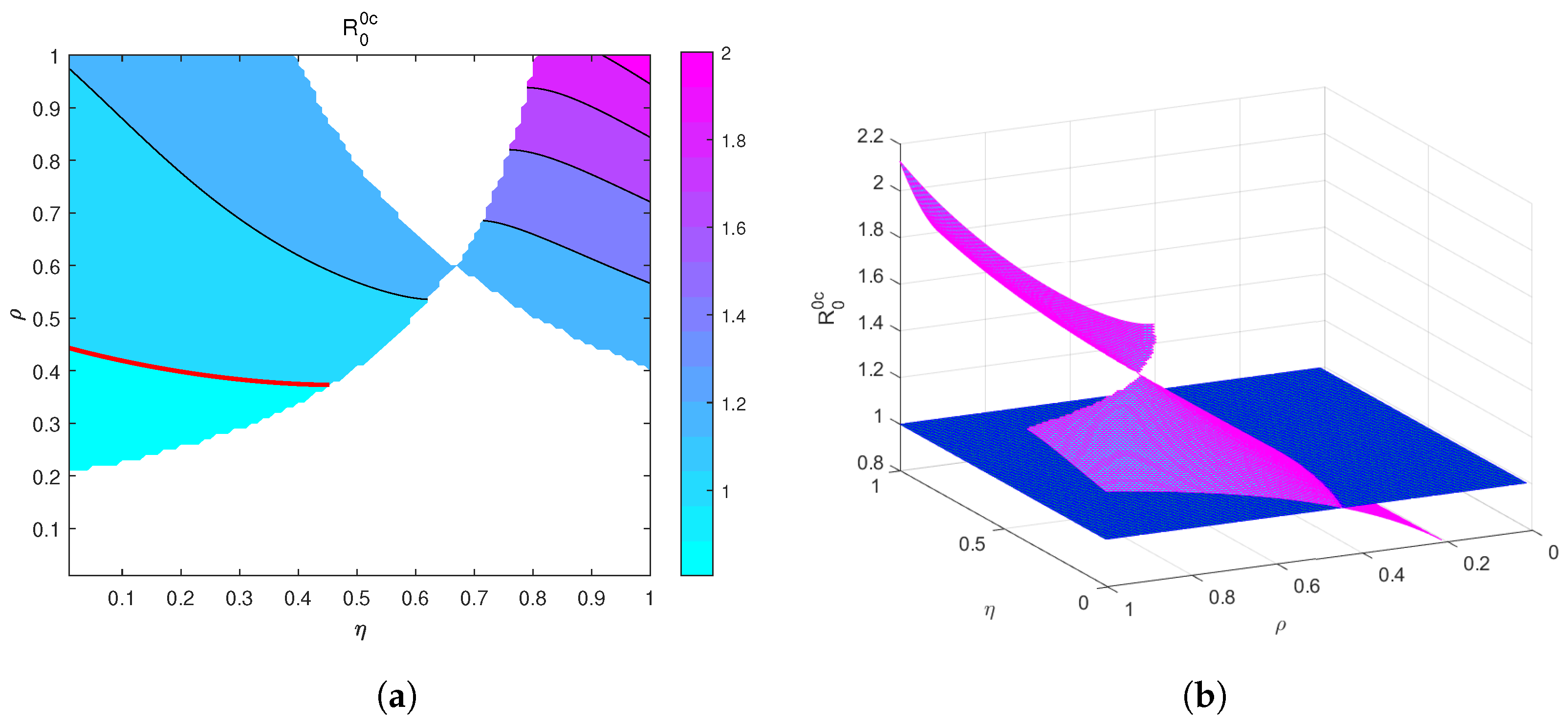
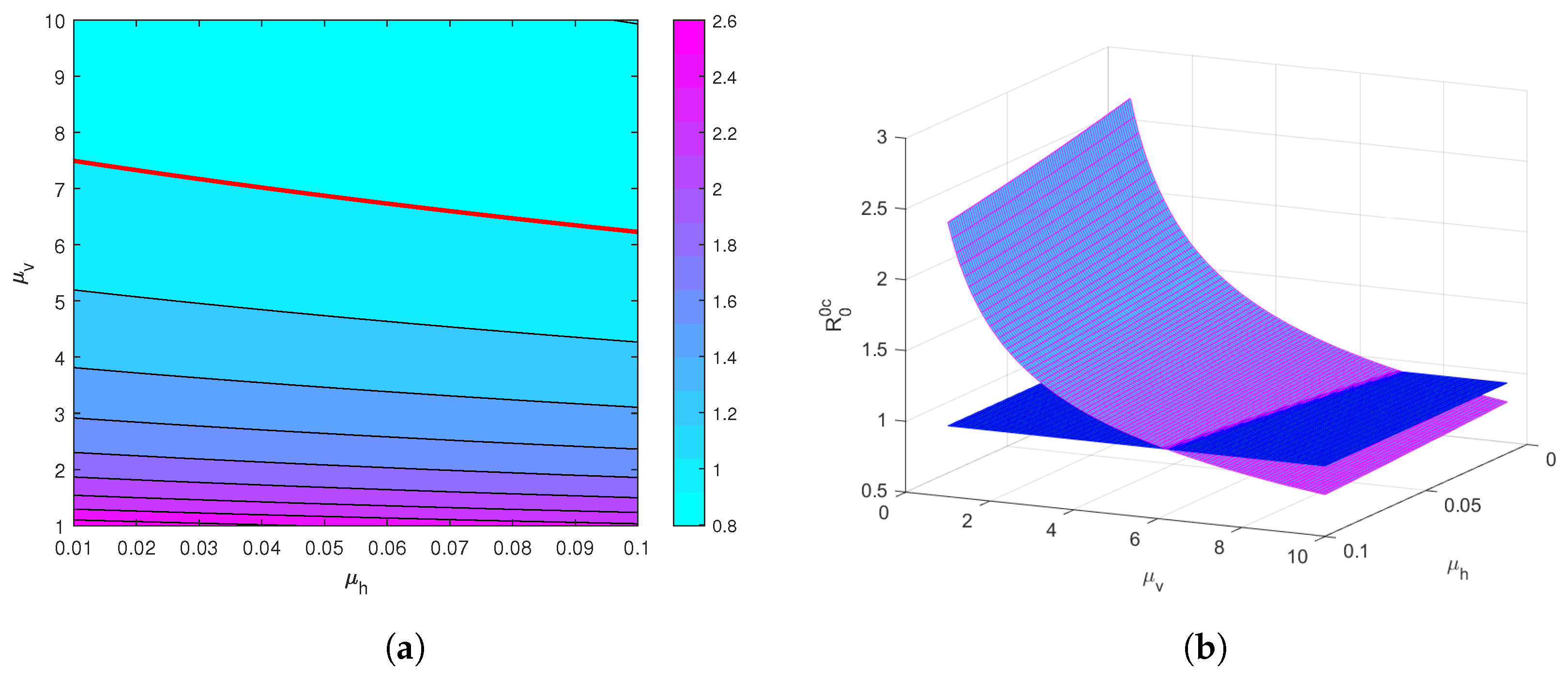
4. Global Sensitivity Analysis of the Reproduction Threshold ${\mathit{R}}_{\mathbf{0}}^{\mathbf{0}\mathit{f}}$

Given the structural complexity of the model and the high degree of uncertainty in estimating many of the input parameters, sensitivity analysis is essential for exploring the behavior of complex models [25]. In this section, we present a sensitivity analysis to evaluate the impact of uncertainty and assess how variations in each parameter of model (2) affect the outcomes of numerical simulations. The analysis employs Latin Hypercube Sampling (LHS) and the Partial Rank Correlation Coefficient (PRCC).

LHS is a statistical technique that employs stratified sampling without replacement. It is particularly effective for analyzing parameter variations across multiple uncertainty ranges for each individual parameter [26]. To generate the LHS matrices, we assumed that all model parameters follow a uniform distribution. We then performed a total of 1000 simulations of the models for each LHS run, using parameter values derived from

Table 2. Parameter values for the HLB model (1).

Parameter	Baseline Values	Unit	Reference
K	1000	−	[27]
$r_h$	$0.6$	0–1	[27]
${\beta }_1$	$0.43$	year−1	[27]
${\mu }_h$	$0.04$	year−1	[27]
$ϵ$	$0.3$	0–1	[12]
${\gamma }_h$	$0.30295$	year−1	[28]
${\mu }_v$	$5.9441$	year−1	[27]
$r_v$	$10{\mu }_v$	year−1	Assumed
m	200	year−1	Assumed
${\beta }_2$	$0.57$	year−1	[27]
$\delta$	$5{\mu }_v$	year−1	Assumed
${\alpha }_1$	3	−	Assumed
${\alpha }_2$	4	−	Assumed
$\rho$	$0.25$	0–1	Assumed
$\eta$	$0.4$	0–1	Assumed

and varying each parameter by $\pm 10\%$ of its value. The Partial Rank Correlation Coefficient (PRCC) measures the strength of the relationship between the model outcomes and the parameters, quantifying the extent to which each parameter influences the outcome [26]. The sensitivity and uncertainty analysis are illustrated in Figure 2, which shows the PRCC values for the parameters of model (2), using the reproduction numbers $R_0^{0c}$ as the function. As depicted in Figure 2a, the parameters negatively affecting the environmental carrying capacity of citrus trees K, the recruitment rate of citrus trees $r_h$, the natural mortality rate of citrus trees ${\mu }_h$, the natural mortality rate of ACP ${\mu }_v$, the roguing rate of infected citrus trees ${\gamma }_h$, the death rate due to insecticides for $SS$ genotype ACP $\delta$, the modification parameter in the natural mortality rate of $RS$ genotype ACP due to fitness cost compared to the natural mortality rate of $SS$ genotype ACP ${\alpha }_1$, and the modification parameter in the natural mortality rate of $RR$ genotype ACP due to fitness cost compared to the natural mortality rate of $SS$ genotype ACP ${\alpha }_2$. Additionally, the recruitment rate of ACP $r_v$, the transmission probability from infected ACP to susceptible citrus tree ${\beta }_1$, the transmission probability from infected citrus trees to susceptible ACP ${\beta }_2$, the probability that a diseased citrus tree sapling is not removed $ϵ$, the average carrying capacity of ACP per citrus tree m, the modification parameter in the death rate of $RS$ genotype ACP due to insecticides compared to the death rate of $RR$ genotype ACP $\eta$, and the modification parameter in the death rate of $RR$ genotype ACP due to insecticides compared to the death rate of $SS$ genotype ACP $\rho$ all positively impact the reproduction number $R_0^{0c}$. For instance, increasing the death rate of ACP can reduce HLB infection, whereas a decrease in parameters such as ${\beta }_1$, ${\beta }_2$, and $r_v$ will lead to a decrease in $R_0^{0c}$. As Figure 2a also shows, the most sensitive parameters are $r_v$, ${\mu }_v$ and $\delta$, followed by the less sensitive parameters such as ${\beta }_1$, ${\beta }_2$, ${\alpha }_1$, ${\alpha }_2$, ${\gamma }_h$, m, and $\rho$. Conversely, $R_0^{0c}$ demonstrates a degree of insensitivity to the parameters K, $r_h$, ${\mu }_h$, $ϵ$, and $\eta$. The identification of these critical parameters is pivotal for formulating effective control strategies that are essential for decreasing the disease prevalence in the grove. Based on the outcomes of the sensitivity analysis, we understand that enhancing the death rate of ACP through insecticide spraying and increasing the removal rate through the roguing of infected trees are two efficient control measures. Regarding the uncertainty analysis, Figure 2b reveals that approximately 72.1% of $R_0^{0c}$ distribution exceeds 1, suggesting a high likelihood of the persistent presence of HLB bacterial infection.

5. Numerical Simulation

In this section, we present numerical simulation results to verify and extend our findings. We explore the impact of insecticide resistance on the transmission of HLB between citrus tree populations and ACP populations and evaluate the effects of various control strategies against HLB. Table 2 provides the parameter values used in these numerical simulations.

We first examine the influence of two model parameters, ${\alpha }_1$ and $\rho$, on the basic reproduction number $R_0^{0c}$ as illustrated in Figure 3. This figure shows how $R_0^{0c}$ varies with the parameters ${\alpha }_1$ and $\rho$. The white areas in Figure 3a indicate that the conditions $g_2>1$ and $(d_3-d_2)(d_3-d_4)>0$ are not satisfied, meaning that $E_{0C}$ does not exist. We observe that $R_0^{0c}$ decreases as ${\alpha }_1$ increases and increases as $\rho$ increases. Figure 3 shows that if the fitness costs of resistance are sufficiently high, it is possible for a large resistance index $\rho$ to result in the basic reproduction number $R_0^{0c}$ less than 1, which could lead to the extinction of ACP. We refer to this phenomenon as the emergence of the paradox.

Figure 4 illustrates how $R_0^{0c}$ varies with parameters ${\alpha }_2$ and $\rho$. The white areas in Figure 4a indicate that the conditions $g_2>1$ and $(d_3-d_2)(d_3-d_4)>0$ are not satisfied, meaning $E_{0C}$ does not exist. We observe that $R_0^{0c}$ decreases as ${\alpha }_2$ increases, while $R_0^{0c}$ increases as $\rho$ increases. As shown in Figure 4, if the fitness cost of resistance is sufficiently high, it is possible for the resistance index $\rho$ to be large while $R_0^{0c}$ remains below 1, leading to the extinction of ACPs. This phenomenon is referred to as the emergence of the paradox.

We analyze the impact of two model parameters, ${\beta }_1$ and ${\beta }_2$ (transmission probabilities between ACP and citrus tree), on the basic reproduction number $R_0^{0c}$ as shown in Figure 5. This figure illustrates how $R_0^{0c}$ changes with variations in ${\beta }_1$ and ${\beta }_2$. It is clear that $R_0^{0c}$ increases with both ${\beta }_1$ and ${\beta }_2$. This implies that a lower transmission probability can help control HLB disease, which is consistent with actual observations.

Figure 6 illustrates how the basic reproduction number $R_0^{0c}$ varies with changes in $\eta$ and $\rho$, where $\rho$ is the parameter that determines the level of dominance of the resistance allele. When $\rho =1$, resistance is dominant, and when $\rho =0$, resistance is recessive. It is evident that $R_0^{0c}$ increases as both $\eta$ and $\rho$ increase. The white areas in Figure 6a indicate the regions where $E_{0C}$ does not exist. Regardless of whether resistance is dominant or recessive, $R_0^{0c}$ increases as the resistance index $\rho$ increases. From Figure 6, it can be seen that when $\rho =1$ (i.e., resistance is is dominant), $R_0^{0c}$ is larger than 1, which means that ACP’s resistance to pesticides is detrimental to HLB control.

Figure 7 illustrates the effect of two model parameters, m and $\delta$, on the basic reproduction number $R_0^{0c}$, where m represents the average carrying capacity of ACP per citrus tree, and $\delta$ represents the additional death rate of ACP due to pesticide exposure. The results show that $R_0^{0c}$ decreases as $\delta$ increases and increases as m increases. Therefore, higher additional mortality due to pesticides and lower carrying capacity of citrus trees are more favorable for the control of HLB.

Figure 8 shows the effect of two model parameters, ${\mu }_h$ (death rate of tree) and ${\mu }_v$ (death rate of ACP), on the basic reproduction number $R_0^{0c}$. From the figure, it is evident that changes in the natural mortality rate of ACP have a more significant impact on $R_0^{0c}$ than changes in the natural mortality rate of citrus trees. Therefore, higher mortality rates of ACP are more favorable for the HLB control.

6. Conclusions

In this paper, we propose a model for HLB dynamics that integrates the population genetics of citrus psyllid vectors to investigate how insecticide use influences the evolution of insecticide resistance at the population level. The model incorporates several features related to HLB transmission dynamics and their correlations: (i) fitness costs associated with insecticide resistance (${\alpha }_1$ and ${\alpha }_2$), including reduced growth rates and increased natural mortality (comparing heterozygous versus homozygous resistant citrus psyllids), and (ii) the dominance of resistance alleles ($\eta$ and $\rho$), which measures the relative sensitivity of heterozygous genotypes to insecticides compared to recessive and dominant genotypes. The main objective of this study is to use mathematical models to understand the impact of insecticide resistance on HLB transmission, particularly to assess whether insecticides can effectively control HLB in epidemic environments.

The epidemiology–genetic model, formulated as a system of nonlinear differential equations, has four disease-free equilibria: a trivial disease-free equilibrium, denoted by $E_{0T}$, where all ACPs are eradicated; a non-trivial sensitive-only disease-free boundary equilibrium, denoted by $E_{0S}$, where $q^{*}=1$ and $p^{*}=0$; a non-trivial resistant-only disease-free boundary equilibrium, denoted by $E_{0R}$, where $q^{*}=0$ and $p^{*}=1$; and a non-trivial co-existence disease-free equilibrium, denoted by $E_{0C}$, where $q^{*}>0$ and $p^{*}>0$. Analysis of the model indicates that the three non-trivial disease-free equilibrium points are locally asymptotically stable when $R_0<1$. In the special case where disease-induced mortality in citrus trees is negligible (i.e., $r_h=0$) and diseased citrus tree saplings are not removed (i.e., $ϵ=1$), the sufficient conditions for the global asymptotical stability of the non-trivial co-existence disease-free equilibrium $E_{0C}$ are established.

We conducted a sensitivity analysis of the model, examining the influence of each parameter on the basic reproduction number using Latin Hypercube Sampling (LHS) and Partial Rank Correlation Coefficient (PRCC). The results indicate that $r_v,{\mu }_v$ and $\delta$ have the most significant impact on the basic reproduction number $R_0^{0c}$. Based on the sensitivity analysis, it is clear that increasing the death rate of Asian citrus psyllids (ACP) through insecticide spraying and enhancing the removal rate of infected trees are two effective control measures.

Finally, numerical simulations were performed to explore the impact of various parameters on HLB transmission between the citrus tree population and the ACP population. The results show that as the fitness cost of resistance increases, the basic reproduction number decreases. Conversely, an increase in the resistance index leads to a higher basic reproduction number. However, if the fitness cost is sufficiently high, a larger resistance index can cause the basic reproduction number to drop below 1, potentially leading to the extinction of the ACP and resulting in a paradoxical effect.

References

1. Batool, A.; Iftikhar, Y.; Mughal, S.; Khan, M.; Jaskani, M.; Abbas, M.; Khan, I. Citrus greening disease-a major cause of citrus decline in the world—A review. Hort. Sci. 2007, 34, 159–166. [Google Scholar] [CrossRef]
2. Inoue, H.; Ohnishi, J.; Ito, T.; Tomimura, K.; Miyata, S.; Iwanami, T.; Ashihara, W. Enhanced proliferation and efficient transmission of Candidatus Liberibacter asiaticus by adult Diaphorina citri after acquisition feeding in the nymphal stage. Ann. Appl. Biol. 2009, 155, 29–36. [Google Scholar] [CrossRef]
3. Marutani-Hert, M.; Hunter, W.B.; Hall, D.G. Establishment of Asian citrus psyllid (Diaphorina citri) primary cultures. Vitr. Cell. Dev. Biol.-Anim. 2009, 45, 317–320. [Google Scholar] [CrossRef] [PubMed]
4. Zhou, C. The status of citrus Huanglongbing in China. Trop. Plant Pathol. 2020, 45, 279–284. [Google Scholar] [CrossRef]
5. Tian, F.; Mo, X.; Rizvi, S.A.H.; Li, C.; Zeng, X. Detection and biochemical characterization of insecticide resistance in field populations of Asian citrus psyllid in Guangdong of China. Sci. Rep. 2018, 8, 12587. [Google Scholar] [CrossRef]
6. Tiwari, S.; Mann, R.S.; Rogers, M.E.; Stelinski, L.L. Insecticide resistance in field populations of Asian citrus psyllid in Florida. Pest Manag. Sci. 2011, 67, 1258–1268. [Google Scholar] [CrossRef]
7. Feyereisen, R. Molecular biology of insecticide resistance. Toxicol. Lett. 1995, 82, 83–90. [Google Scholar] [CrossRef]
8. Tiwari, S.; Gondhalekar, A.; Mann, R.; Scharf, M.; Stelinski, L. Characterization of five CYP4 genes from Asian citrus psyllid and their expression levels in Candidatus Liberibacter asiaticus-infected and uninfected psyllids. Insect Mol. Biol. 2011, 20, 733–744. [Google Scholar] [CrossRef]
9. Tiwari, S.; Pelz-Stelinski, K.; Mann, R.S.; Stelinski, L.L. Glutathione transferase and cytochrome P450 (general oxidase) activity levels in Candidatus Liberibacter asiaticus-infected and uninfected Asian citrus psyllid (Hemiptera: Psyllidae). Ann. Entomol. Soc. Am. 2011, 104, 297–305. [Google Scholar] [CrossRef]
10. Yu, X.; Killiny, N. RNA interference of two glutathione S-transferase genes, Diaphorina citri DcGSTe2 and DcGSTd1, increases the susceptibility of Asian citrus psyllid (Hemiptera: Liviidae) to the pesticides fenpropathrin and thiamethoxam. Pest Manag. Sci. 2018, 74, 638–647. [Google Scholar] [CrossRef]
11. Liang, J.; Tang, S.; Nieto, J.J.; Cheke, R.A. Analytical methods for detecting pesticide switches with evolution of pesticide resistance. Math. Biosci. 2013, 245, 249–257. [Google Scholar] [CrossRef] [PubMed]
12. Tang, S.; Gao, S.; Zhang, F.; Liu, Y. Role of vector resistance and grafting infection in Huanglongbing control models. Infect. Dis. Model. 2023, 8, 491–513. [Google Scholar] [CrossRef]
13. Luo, Y.; Zhang, F.; Liu, Y.; Gao, S. Analysis and optimal control of a Huanglongbing mathematical model with resistant vector. Infect. Dis. Model. 2021, 6, 782–804. [Google Scholar] [CrossRef] [PubMed]
14. Griffiths, A.J.; Wessler, S.R.; Lewontin, R.C.; Carroll, S.B. Introduction to Genetic Analysis (Loose-Leaf); Macmillan: New York, NY, USA, 2008. [Google Scholar]
15. Freeman, S.; Herron, J.C. Evolutionary Analysis; Pearson Prentice Hall: Upper Saddle River, NJ, USA, 2007. [Google Scholar]
16. Kuniyoshi, M.L.G.; Santos, F.L.P.d. Mathematical modelling of vector-borne diseases and insecticide resistance evolution. J. Venom. Anim. Toxins Incl. Trop. Dis. 2017, 23, 34. [Google Scholar] [CrossRef]
17. Mohammed-Awel, J.; Gumel, A.B. Mathematics of an epidemiology-genetics model for assessing the role of insecticides resistance on malaria transmission dynamics. Math. Biosci. 2019, 312, 33–49. [Google Scholar] [CrossRef]
18. Bourguet, D.; Genissel, A.; Raymond, M. Insecticide resistance and dominance levels. J. Econ. Entomol. 2000, 93, 1588–1595. [Google Scholar] [CrossRef]
19. Hastings, A. Population Biology: Concepts and Models; Springer Science & Business Media: Berlin/Heidelberg, Germany, 2013. [Google Scholar]
20. Luz, P.; Codeco, C.; Medlock, J.; Struchiner, C.; Valle, D.; Galvani, A. Impact of insecticide interventions on the abundance and resistance profile of Aedes aegypti. Epidemiol. Infect. 2009, 137, 1203–1215. [Google Scholar] [CrossRef] [PubMed]
21. Alout, H.; Dabiré, R.K.; Djogbénou, L.S.; Abate, L.; Corbel, V.; Chandre, F.; Cohuet, A. Interactive cost of Plasmodium infection and insecticide resistance in the malaria vector Anopheles gambiae. Sci. Rep. 2016, 6, 29755. [Google Scholar] [CrossRef]
22. Anderson, R.A.; Knols, B.; Koella, J. Plasmodium falciparum sporozoites increase feeding-associated mortality of their mosquito hosts Anopheles gambiae sl. Parasitology 2000, 120, 329–333. [Google Scholar] [CrossRef]
23. Barbosa, S.; Hastings, I.M. The importance of modelling the spread of insecticide resistance in a heterogeneous environment: The example of adding synergists to bed nets. Malar. J. 2012, 11, 258. [Google Scholar] [CrossRef]
24. Van den Driessche, P.; Watmough, J. Reproduction numbers and sub-threshold endemic equilibria for compartmental models of disease transmission. Math. Biosci. 2002, 180, 29–48. [Google Scholar] [CrossRef] [PubMed]
25. Blower, S.M.; Dowlatabadi, H. Sensitivity and uncertainty analysis of complex models of disease transmission: An HIV model, as an example. Int. Stat. Rev./Rev. Int. Stat. 1994, 62, 229–243. [Google Scholar] [CrossRef]
26. Agusto, F.; Khan, M. Optimal control strategies for dengue transmission in Pakistan. Math. Biosci. 2018, 305, 102–121. [Google Scholar] [CrossRef] [PubMed]
27. Zhang, F.; Qiu, Z.; Zhong, B.; Feng, T.; Huang, A. Modeling Citrus Huanglongbing transmission within an orchard and its optimal control. Math. Biosci. Eng. 2020, 17, 2048–2069. [Google Scholar] [CrossRef]
28. Taylor, R.A.; Mordecai, E.A.; Gilligan, C.A.; Rohr, J.R.; Johnson, L.R. Mathematical models are a powerful method to understand and control the spread of Huanglongbing. PeerJ 2016, 4, 2642–2660. [Google Scholar] [CrossRef]
Figure 1. Schematic diagram of the HLB model (1).
Computation 12 00242 g001
Figure 2. Sensitivity analysis and uncertainty analysis of the basic reproduction number R 0 0 c . (a) shows the sensitivity indices of R 0 0 c , and (b) shows the histogram obtained from LHS using a sample size of 1000 for R 0 0 c .
Computation 12 00242 g002
Figure 3. The relationship graphs between R 0 0 c and parameters α 1 and ρ : (a) contour map, (b) three-dimensional map. The red curve indicates that the basic regeneration number R 0 0 c is equal to one.
Computation 12 00242 g003
Figure 4. The relationship graphs between R 0 0 c and parameters α 2 and ρ : (a) contour map, (b) three-dimensional map. The red curve indicates that the basic regeneration number R 0 0 c is equal to one.
Computation 12 00242 g004
Figure 5. The relationship graphs between R 0 0 c and parameters β 1 and β 2 : (a) contour map, (b) three-dimensional map. The red curve indicates that the basic regeneration number R 0 0 c is equal to one.
Computation 12 00242 g005
Figure 6. The relationship graphs between R 0 0 c and parameters η and ρ : (a) contour map, (b) three-dimensional map. The red curve indicates that the basic regeneration number R 0 0 c is equal to one.
Computation 12 00242 g006
Figure 7. The relationship graphs between R 0 0 c and parameters m and δ : (a) contour map, (b) three-dimensional map. The red curve indicates that the basic regeneration number R 0 0 c is equal to one.
Computation 12 00242 g007
Figure 8. The relationship graphs between R 0 0 c and parameters μ h and μ v : (a) contour map, (b) three-dimensional map. The red curve indicates that the basic regeneration number R 0 0 c is equal to one.
Computation 12 00242 g008