Abstract
The fusion process considers the boundary between correct and conflict records. It has been a fundamental component in ensuring the accuracy of many mathematical algorithms that utilize multiple input sources. Fusion techniques give priority and high weight to reliable and qualified sources since their information is most likely to be trustworthy. This study stochastically investigates the three most common fusion techniques: Kalman filtering, particle filtering and Bayesian probability (which is the basis of other techniques). The paper focuses on using fusion techniques in the context of state estimation for dynamic systems to improve reliability and accuracy. The fusion methods are investigated using different types of datasets to find out their performance and accuracy in state estimation.
1. Introduction
Obtaining knowledge from a single source may or may not be precise depending on the quality of the source. Therefore, gathering information from different sources is more beneficial to find the accurate result, and this process is called data fusion. Data fusion is a specific type of data integration that merges various sources to obtain a comprehensive and trustworthy result [1,2]. It is more specific than data integration in that it does not just bring all the information together; instead, it enhances and obtains a clear conception of the required data. There are many types of fusion, such as data fusion, which is defined by Dong et al. (2014) as gathering information from different websites, posts, blogs, or databases to obtain a highly reliable outcome [3]. On the other hand, sensor fusion, as discovered by Hall and Llinas in 1997, involves the integration of data from multiple sensors, such as cameras, radar, or LIDAR, which typically exhibit significant conflicts and high levels of noise [4]. Thus, sensor fusion aims to enhance the quality of data by filtering out noise and errors [5]. The goal of both types is to produce complete and error-free recorders, which cannot be achieved by using only a single source or sensor. Sensor and data fusion have been applied intensively in recent years. Many fields, such as education, military, medicine, and even emergency cases, rely on fusion techniques to make the final decision. For instance, to save people’s lives in emergencies, such as earthquakes or floods, real-time image fusion considers the best way to rescue people as fast as possible. Also, in medical cases using multisensors along with image fusion brings a great benefit in retrieving information autonomously, especially the data that is difficult to be seen by humans [6]. Currently, even robot state estimation relies completely on fusion techniques to derive the accurate estimation of variables [7]. These dynamic robots need fusion techniques to move smoothly, avoiding all the obstacles that are in their path. Therefore, intensive research has been performed in recent years to find the best fusion algorithm for state estimation.
In this work, we have focused on using fusion techniques to estimate the state of a dynamic system using different types of experiments. In Section 2, we studied fusion algorithms stochastically and compared their accuracy, consistency, robustness, and scalability. Section 3 contains information about the datasets that we used. In Section 4, we showed the results of the fusion after applying the algorithms using different datasets. Section 5 shows the evaluation of the used algorithms using MAE and RMSE metrics. Finally, the last section contains the conclusion and future work.
2. Fusion Algorithms
There are different types of data fusion algorithms and their popularity changes depending on the problem domain and requirements. However, some of the algorithms are widely known and can be used in many fields, as described below.
2.1. Particle Filtering
Particle filtering (PF), which is also known as the sequential Monte Carlo algorithm, is used to solve complex nonlinear filtering problems [8,9,10]. It is considered to be the alternative to extended Kalman filtering and the unscented Kalman filter. It was first developed by Genshiro Kitagawa in 1993 to fuse dynamic system data [11]. It is called particle filtering since it uses particles or samples for estimation processes, based on a series of observations. The work of PF can be summarized as a method to estimate the system’s state over time. If we assign the variable k to the time step, then, for the estimated state, we assign at k time step. Thus, the change in the state estimation in each time step can be represented by using the following probability equation:
Each time the calculation of the measurements takes place, it is denoted as . So, to model these measurements, the probability distribution can be represented by
where means the likelihood or probability density of observing , given . After that, we generate n particles at each time step k, by sampling from prior state distribution P(Xk|Xk−1). For each particle, we calculate the weight by the likelihood of the observed data. So, a particle’s weight can be computed by
That means the particles obtains higher weights if they are more consistent with the observed measurement . The particle that gains a high weight is usually transferred to the next time step, and this step is called the resampling step. This aids in focusing on the high weight particles representing the state of the system. Finally, the final state estimation is performed by using the following model in time step k:
The continuous iteration process, using particle filtering, updates particles in each time step k, which shows the estimated state for the dynamic system. This is what makes particle filtering effective in dealing with complex nonlinear systems.
2.2. Kalman Filtering
Kalman filtering (KF) is one of the best fusion techniques nowadays, especially for fusing noisy sensors. KF was defined in 1960 by the Hungarian scientist Rudolf E. Kalman [12]. In simple terms, KF uses a noisy and inconsistent input and produces a clear and consistent output. The fusion process starts by defining a mathematical model that describes how the system evolves over time. Then, the filtering process takes place depending on the initial state and some measurements. Those measurements are provided by different sensors to describe the relationship between them and the state of the system, which is predominantly noisy and conflicting. Afterwards, the prediction for the new state estimation and evolution over time is established using the system model and the estimated state. It also involves updating the covariance matrix of the associated states. The final step includes updating the state estimation by combining the sensor measurement and the predicted state estimation and updating the state covariance matrix as well. During the update process, Kalman filtering assigns weights to each sensor measurement depending on its reliability and certainty. Thus, the best sensor obtains the highest weight, and the worst sensor obtains the lowest weight. To decompose KF into its component stochastically, we then describe the state as the probabilistic variable X. Thus, at time step k it is represented as . The mean is represented as and the covariance is represented as to represent the probability distribution. Thus, the state transition can be written as
where A and B are used to represent the system dynamics, U(k) represents the control input, and represents the noise.
Now, we come to the representation of the measurement stochastically at time step k as . In this case, the mean can be symbolized as and the covariance matrix of the measurement noise as to show the uncertainty in the measurement. Thus, the measurement model can be written as
where H is the measurement matrix, while is the noise. In the prediction step, the state estimation is stochastically represented as and the covariance is represented as . In the update step, as mentioned above, the predicted state estimation is combined with the actual measurement. So, the representation of the updated state estimation is described as and the covariance is described as which can be calculated as follows:
where I is the identical matrix and is the Kalman gain, which can be calculated as follows:
At each time step, this model helps in providing probabilistic estimation to get rid of the noise and uncertainty problems. The main objective of Kalman filtering is to minimize the MSE between the true state and the estimated one. However, it has one drawback of working only with a linear system and Gaussian noise. Therefore, other types of Kalman filtering, such as extended Kalman filtering (EKF) and unscented Kalman filtering (UKF) were developed to deal with non-linear systems [13].
2.2.1. Extended Kalman Filtering
Extended Kalman filtering is a subset of Kalman filtering but works mostly with non-linear systems [14,15,16,17]. It works perfectly for fusion sensors, providing highly reliable records. The EKF procedure consists of similar stages as KF. In the beginning, the state X and its covariance P are supposed to be determined. After that, the algorithm defines the process model with the noise P and the measurement matrix of noise with R. The prediction of each event state , using the process model and random noise , can be calculated by
where f represents the nonlinear state transition, and A and B represents the system dynamics. Now, to represent the measurement at time step k as , then
where h represents nonlinear measurement model, H represents measurement matrix, and represents the measurement noise. Note that EKF uses Jacobian matrices to linearize f and h.
In the update step as it mentioned above, the predicted state estimation combines with the actual measurement. So, the representation of the updated state estimation can be calculated as
where K is the Kalman gain that can be obtained from Equation (9), while the covariance can be calculated using Equation (8).
Lastly, the algorithm repeatedly predicts and updates the state estimation for each time step. The outcome from the iteration process considers the best state estimation of the required event.
2.2.2. Unscented Kalman Filtering
UKF is also a subset of KF, used as a standard technique for estimating states in nonlinear cases. It was defined for the first time by the robotics research group Simon J. Julior and Jeffery K. Uhlmann in 1997 [18]. This algorithm has many advantages compared to the standard KF and EKF in performing high accurate outcomes and reducing computational complexity. In the stochastic sensor and data fusion context, the steps using UKF start by initializing the state vector X and the covariance matrix P. After that, the algorithm defines the process model with the noise Q and the measurements with the noise R. To capture the nonlinearity, UKF uses a set of sigma points [19,20]. Those points are selected depending on the mean of X and the covariance of P. To begin with the prediction process, the algorithm calculates the prediction of the state sigma point in the advance suing process model F, with the control input U, and the process noise W:
while, to represent the measurement at time step k as , then
In the update step as mentioned above, the predicted state estimation combines with the actual measurement. So, the representation of the updated state estimation described as can be calculated using Equation (12), and covariance can be calculated by Equation (8).
The algorithm repeatedly predicts and updates the state estimation for each time step. The final decided state estimation considers the best prediction of the required event. To get rid of the explicit linearization, UKF uses sigma points to obtain the state and measurement distributions.
The main difference between KF, EKF, and UKF, is that each one of them addresses the limitation of the previous version. For more details, KF is an optimal algorithm to estimate the state only when the system is linear, and the noise is Gaussian. However, the EKF deals with non-linear systems by linearizing them around the current state using the Jacobian matrix. This is why EKF is more effective than KF. But it still has some limitations, especially that the linearization process introduces errors and using the Jacobian matrix increases the computational complexity. These limitations can be addressed using UKF, which deals with non-linear systems without linearizing them; instead, it uses sigma points. Also, it reduces computational complexity by using sigma points rather than the Jacobian matrix in estimating the state.
2.3. Bayesian Probability
Bayesian probability is based on Bayes’s theorem. It explains the relationship between the prior probability distribution and the posterior probability distribution of an event or belief using evidence [21]. BP has been used widely in data and sensor fusion to obtain more robust and accurate decisions. Since each source provides data with a potential noise, BP helps in getting rid of uncertainty by fusing those sources. The steps of fusion using BP start by defining the system model at a given time k which is denoted as . If the state of the object changes by time, then it can be described by a probability distribution as . Each of these sources provide measurements with inherent noise. The relationship between those measurements and the real state of the object described as . The two essential steps in BP are predict and update processes. In predict process, the state at time k can be predict by:
The update step involves a state estimation update using the recent measurements:
The steps for predicting and updating are iterated in each time step, and the state estimation updates whenever new measurements show during the iteration. The final process is to estimate the next state using either Kalman filtering for linear systems or particle filtering for nonlinear and non-Gaussian systems. To rephrase, we could use BP alone, but combining it with KF or PF can bring many advantages. Using BP alone poses challenges when the system is complexly dynamic and when the noise is non-Gaussian. So, we use KF to handle non-Gaussian noise and PF when the system is non-linear. This combination leads to more accurate state estimation.
In short, Bayesian filtering is a probabilistic approach that is used often nowadays for object tracking and computer vision cases in stochastic environments. It has a great ability to deal with noises and treat them, while combining data from different sources. Bayesian probability usually works to predict and update individual probabilities. However, there is an extended version of this theory that deals with more complex dependencies between the variables called the Bayesian network.
Bayesian Network
The Bayesian network, also called the probabilistic graphical model, is defined by Judea Pearl (1988) as showing the relationship between a set of variables using directed acyclic graphs [22]. It constitutes a subset of Bayesian probability. It has been used widely in the last few years to solve uncertainty problems in many fields, like artificial intelligence and data fusion [23]. It has a great ability for fusing information coming from different sources to distinguish between correct and incorrect data. A BN consists of nodes and edges. Nodes are the inserted variables that can be discrete or continuous, while the edges are the probabilistic relationships between those variables [24]. After defining the variables, conditional distribution is specified for each node. Since the source has various degrees of accuracy, then each source must have a different conditional probabilistic table (CPT). In a BN, each node X has specific CPT given by its parent . The CPT can be described as . On the other hand, the joint probability distribution for all the nodes can be described as
After constructing the BN, Bayesian inference is performed to calculate the posterior probability of each variable. Given the evidence from the source, the calculation of posterior probability performed by Bayesian theorem is as follows:
where is the posterior probability of X given E (evidence) and is the prior probability of X, while is the marginal probability of all evidence.
After these steps, updating the probability distribution for each variable should be carried out. This helps in building models to fuse data from uncertainty and ambiguity.
3. Datasets
In our experiments, we used two types of datasets to simulate the position of a dynamic object, such as a robot. Initially, we utilized a toy dataset, which took the positions [2.0, 3.0, 4.0, 5.0, 6.0, 7.0, 8.0], consecutively. Then, we used a synthetic dataset of 1000 positions. The reason for using a synthetic dataset was to figure out the performance of the estimation algorithms that we used. We applied a sequence of values starting at 0 and ending at 20, with 1000 positions between them, as shown in the following one-dimensional array:
True position: [0, 0.02002002, 0.04004004, 0.06006006, 0.08008008, 0.1001001, ……, 19.93993994, 19.95995996, 19.97997998, 20].
This considers the ground truth of dynamic objects from 0 to 20 having 1000 time steps.
4. State Estimation
In this paper, we applied the algorithms PF, KF, EKF, UKF, and BP, which are mentioned above, to estimate the state of a dynamic object. Firstly, we used a toy dataset of a moving object like a robot, then we used a synthetic dataset. Secondly, we applied fusion algorithms to estimate those positions correctly without having conflicts. We applied a particle filtering algorithm by using 100 particles. We added 0.5 noise to the measurements of the true position, and we used a constant velocity model to see the particles evolve over time. Accordingly, the calculation of the particle’s weight depending on the estimation of its measurements, as mentioned in Section 2.3, took place. At the end, we resampled to retain only the best particles, which helped in obtaining the final estimated state values, as shown in Figure 1, where the blue line represents the true position, and the orange one represents the estimated positions.
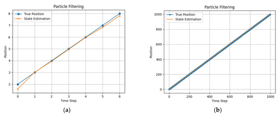
Figure 1.
The true position and the state estimation with PF (a) using a toy dataset and (b) using a large dataset.
Secondly, we applied the Kalman filtering algorithm using the same datasets. We added 0.5 noise to the measurement of the true positions. Then, we configured Kalman filtering, with its parameters and conditions. Performing a KF iteration with each measurement is necessary to obtain good state estimation. The performance of KF is shown in Figure 2. Additionally, we applied EKF and UKF using the same datasets to estimate the state of the dynamic system, as shown in Figure 3 and Figure 4. Figure 5 illustrates the estimation using BP, with the same datasets
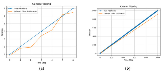
Figure 2.
The true position and the state estimation with KF (a) using a toy dataset and (b) using a large dataset.
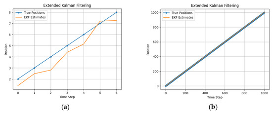
Figure 3.
The true position and the state estimation with EKF (a) using a toy dataset and (b) using a large dataset.
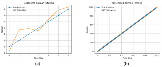
Figure 4.
The true position and the state estimation with UKF (a) using a toy dataset and (b) using a large dataset.
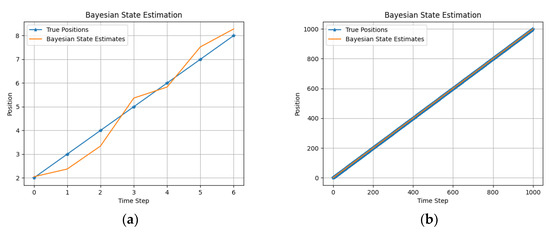
Figure 5.
The true position and the state estimation with BP (a) using a toy dataset and (b) using a large dataset.
5. Experiments and Evaluation
To validate the models, we used the mean absolute error (MAE), which is the absolute value of the difference between the true position of the object and the estimated one [25], and the root mean square error (RMSE), which is the average measurement of the square differences between the true position of the object and the estimated state. Table 1 shows the result of the RMSE and MAE of PF, KF, EKF, UKF, and BP using a toy dataset and a synthetic dataset.

Table 1.
The result of MAE and RMSE using fusion algorithms.
In the case of the toy dataset, PF showed the best result in contrast to other algorithms as shown in Table 2. But, while using a large dataset, the UKF performed significantly better. Using a large dataset showed a higher accuracy for all the algorithms. However, UKF showed superior results compared to other algorithms, even while using higher noise rates.

Table 2.
Estimated states for toy dataset using fusion algorithms.
6. Conclusions
Autonomous state estimation has become a center of attention for many scientists since it is essential in many robust cases. Fusion algorithms have the efficient ability to estimate the state of dynamic systems. In this paper, we evaluated the performance of fusion algorithms, such as Kalman filtering, which works with mostly linear systems. Also, we used extended Kalman filtering and unscented Kalman filtering to deal with non-linear systems and address the limitations of KF. Moreover, we used particle filters, which showed superior results when working with toy datasets. Lastly, we used Bayesian probability which is the basis of fusion algorithms. Then, we presented the outcomes using two experiments: the first one used a toy dataset and the second one used a synthetic dataset. For the evaluation, we used MAE and RMSE to see the difference between the true position and the estimated one. The evaluation of the algorithms showed a high accuracy with lowest error rate, especially while using a large dataset. The UKF outperformed all the other algorithms, particularly when applied to a large dataset. It obtained the lowest MAE of 0.2751082709 and an RMSE of 0.3431953125. This study represents the initial phase of our research. We intend to extend this research, using these algorithms to track drones in real-world experiments.
Author Contributions
Conceptualization, A.H.A. and H.T.; methodology, A.H.A.; software, A.H.A.; validation, A.H.A. and H.T.; formal analysis, A.H.A.; investigation, A.H.A.; resources, A.H.A. and H.T.; data curation, A.H.A.; writing—original draft preparation, A.H.A.; writing—review and editing, A.H.A. and H.T.; visualization, A.H.A. and H.T.; supervision, H.T.; funding acquisition, H.T. All authors have read and agreed to the published version of the manuscript.
Funding
This work was supported by the University of Debrecen Program for Scientific Publication.
Data Availability Statement
Dataset available upon request to the authors.
Conflicts of Interest
The authors declare no conflicts of interest.
Nomenclature
| Symbols | Description |
| PF | Particle filtering |
| K | Time step |
| Xk | Estimated state at k time step |
| Zk | Measurements at k time step |
| Particle’s weight at k time step | |
| KF, EKF, UKF | Kalman filtering, extended Kalman filtering, unscented Kalman filtering |
| A, B | Representors of system dynamic |
| U(K) | The control input |
| W(K), V(K) | Random noise |
| H, I | Measurement matrix, identical matrix |
| f | Nonlinear state transition |
| h | Nonlinear measurement model |
| K | Kalman gain |
| P | Covariance matrix |
| BP, BN | Bayesian probability, Bayesian network |
| CPT | Conditional probabilistic table |
| Posterior probability of X given E | |
| P(x) | Prior probability of X |
| Marginal probability of all evidence |
References
- Ahmed, A.H.; Sadri, F. Datafusion: Taking source confidences into account. In Proceedings of the 8th International Conference on Information Systems and Technologies, Istanbul, Turkey, 16–18 March 2018. [Google Scholar] [CrossRef]
- Pochampally, R.; Das Sarma, A.; Dong, X.L.; Meliou, A.; Srivastava, D. Fusing data with correlations. In Proceedings of the SIGMOD ’14: Proceedings of the 2014 ACM SIGMOD International Conference on Management of Data, Snowbird, UT, USA, 22–27 June 2014. [Google Scholar] [CrossRef]
- Dong, X.L.; Gabrilovich, E.; Heitz, G.; Horn, W.; Murphy, K.; Sun, S.; Zhang, W. From data fusion to knowledge fusion. Proc. Vldb Endow. 2014, 7, 881–892. [Google Scholar] [CrossRef]
- Hall, D.; Llinas, J. An introduction to multisensor data fusion. Proc. IEEE 1997, 85, 6–23. [Google Scholar] [CrossRef]
- Yeong, D.J.; Velasco-Hernandez, G.; Barry, J.; Walsh, J. Sensor and sensor fusion technology in autonomous vehicles: A review. Sensors 2021, 21, 2140. [Google Scholar] [CrossRef]
- Canalle, G.K.; Salgado, A.C.; Loscio, B.F. A survey on data fusion: What for? in what form? what is next? J. Intell. Inf. Syst. 2020, 57, 25–50. [Google Scholar] [CrossRef]
- Doumbia, M.; Cheng, X. State Estimation and localization based on sensor fusion for autonomous robots in indoor environment. Computers 2020, 9, 84. [Google Scholar] [CrossRef]
- Wills, A.G.; Schön, T.B. Sequential Monte Carlo: A unified review. Annu. Rev. Control. Robot. Auton. Syst. 2023, 6, 159–182. [Google Scholar] [CrossRef]
- Djuric, P.; Kotecha, J.; Zhang, J.; Huang, Y.; Ghirmai, T.; Bugallo, M.; Miguez, J. Particle filtering. IEEE Signal Process. Mag. 2003, 20, 19–38. [Google Scholar] [CrossRef]
- Sekehravani, E.A.; Babulak, E.; Masoodi, M. Flying object tracking and classification of military versus nonmilitary aircraft. Bull. Electr. Eng. Inform. 2020, 9, 1394–1403. [Google Scholar] [CrossRef]
- Kitagawa, G. Monte Carlo Filtering and smoothing for nonlinear NON-Gaussian state space model. In Proceedings of the ISCIE International Symposium on Stochastic Systems Theory and Its Applications, Online, 28 May 1998; Volume 1998, pp. 1–6. [Google Scholar] [CrossRef]
- Urrea, C.; Agramonte, R. Kalman Filter: Historical Overview and Review of Its Use in Robotics 60 Years after Its Creation. J. Sensors 2021, 2021, 9674015. [Google Scholar] [CrossRef]
- Goh, S.T.; Zekavat, S.A.; Abdelkhalik, O. An introduction to Kalman filtering implementation for localization and tracking applications. In Handbook of Position Location; Wiley: Hoboken, NJ, USA, 2018; pp. 143–195. [Google Scholar]
- Chadha, H.S. Extended Kalman Filter: Why do we need an Extended Version? Medium. 16 December 2019. Available online: https://towardsdatascience.com/extended-kalman-filter-43e52b16757d (accessed on 7 April 2018).
- Lagraoui, M.; Nejmi, A.; Rayhane, H.; Taouni, A. Estimation of lithium-ion battery state-of-charge using an extended kalman filter. Bull. Electr. Eng. Inform. 2021, 10, 1759–1768. [Google Scholar] [CrossRef]
- Kamarposhti, M.A.; Solyman, A.A.A. The estimate of amplitude and phase of harmonics in power system using the extended kalman filter. Bull. Electr. Eng. Inform. 2021, 10, 1785–1792. [Google Scholar] [CrossRef]
- Kirad, A.; Groini, S.; Soufi, Y. Improved sensorless backstepping controller using extended Kalman filter of a permanent magnet synchronous machine. Bull. Electr. Eng. Inform. 2022, 11, 658–671. [Google Scholar] [CrossRef]
- Julier, S.; Uhlmann, J. New extension of the Kalman filter to nonlinear systems. In Signal Processing, Sensor Fusion, and Target Recognition VI; SPIE: Weinheim, Germany, 1997. [Google Scholar] [CrossRef]
- György, K.; Kelemen, A.; Dávid, L. Unscented kalman filters and particle filter methods for nonlinear state estimation. Procedia Technol. 2014, 12, 65–74. [Google Scholar] [CrossRef]
- Wan, E.A.; Van Der Merwe, R. The unscented Kalman filter for nonlinear estimation. In Proceedings of the IEEE 2000 Adaptive Systems for Signal Processing, Communications, and Control Symposium (Cat. No.00EX373), Lake Louise, AB, Canada, 4 October 2000; pp. 153–158. [Google Scholar]
- van de Schoot, R.; Depaoli, S.; King, R.; Kramer, B.; Märtens, K.; Tadesse, M.G.; Vannucci, M.; Gelman, A.; Veen, D.; Willemsen, J.; et al. Bayesian statistics and modelling. Nat. Rev. Methods Prim. 2021, 1, 1–26. [Google Scholar] [CrossRef]
- Imoto, S.; Matsuo, H.; Miyano, S. Gene Networks: Estimation, Modeling, and Simulation; Elsevier: Amsterdam, The Netherlands, 2014; pp. 89–112. [Google Scholar] [CrossRef]
- Bielza, C.; Larraã±Aga, P. Bayesian networks in neuroscience: A survey. Front. Comput. Neurosci. 2014, 8, 131. [Google Scholar] [CrossRef]
- Ibeni, W.N.L.W.H.; Salikon, M.Z.M.; Mustapha, A.; Daud, S.A.; Salleh, M.N.M. Comparative analysis on bayesian classification for breast cancer problem. Bull. Electr. Eng. Inform. 2019, 8. [Google Scholar] [CrossRef]
- Chollet, F. Deep Learning with Python, 2nd ed.; Simon and Schuster: New York, NY, USA, 2021. [Google Scholar]
Disclaimer/Publisher’s Note: The statements, opinions and data contained in all publications are solely those of the individual author(s) and contributor(s) and not of MDPI and/or the editor(s). MDPI and/or the editor(s) disclaim responsibility for any injury to people or property resulting from any ideas, methods, instructions or products referred to in the content. |
© 2024 by the authors. Licensee MDPI, Basel, Switzerland. This article is an open access article distributed under the terms and conditions of the Creative Commons Attribution (CC BY) license (https://creativecommons.org/licenses/by/4.0/).