The Efficacy of Multi-Period Long-Term Power Transmission Network Expansion Model with Penetration of Renewable Sources

Abstract

The electrical energy demand increase does evolve rapidly due to several socioeconomic factors such as industrialisation, population growth, urbanisation and, of course, the evolution of modern technologies in this 4th industrial revolution era. Such a rapid increase in energy demand introduces a huge challenge into the power system, which has paved way for network operators to seek alternative energy resources other than the conventional fossil fuel system. Hence, the penetration of renewable energy into the electricity supply mix has evolved rapidly in the past three decades. However, the grid system has to be well planned ahead to accommodate such an increase in energy demand in the long run. Transmission Network Expansion Planning (TNEP) is a well ordered and profitable expansion of power facilities that meets the expected electric energy demand with an allowable degree of reliability. This paper proposes a DC TNEP model that minimises the capital costs of additional transmission lines, network reinforcements, generator operation costs and the costs of renewable energy penetration, while satisfying the increase in demand. The problem is formulated as a mixed integer linear programming (MILP) problem. The developed model was tested in several IEEE test systems in multi-period scenarios. We also carried out a detailed derivation of the new non-negative variables in terms of the power flow magnitudes, the bus voltage phase angles and the lines’ phase angles for proper mixed integer variable decomposition techniques. Moreover, we intend to provide additional recommendations in terms of in which particular year (within a 20 year planning period) can the network operators install new line(s), new corridor(s) and/or additional generation capacity to the respective existing power networks. This is achieved by running incremental period simulations from the base year through the planning horizon. The results show the efficacy of the developed model in solving the TNEP problem with a reduced and acceptable computation time, even for large power grid system.

1. Introduction

1.1. Motivation

Transmission network expansion planning (TNEP) is one of the major strategic decisions in power system planning and optimisation, where the expansion of the existing network is the primary purpose. The act is carried out by integrating new generation units, reinforcing the existing power lines, creating new transmission corridors and/or adding new power lines to prepare for the increasing future energy demands, in view of maintaining the system’s reliability and efficiency [1,2,3,4]. However, the improved reliability in the high quality energy supply must correlate with the available funds [5,6,7].

TNEP also has a crucial aspect, which is the integration of renewable energy generation units to form a large-scale grid system to satisfy the high demand in energy [8,9]. The integration of renewable energy sources to the grid is crucial due to the clean energy needs to meet the emission reduction targets [10]. However, the renewable energy intermittent behaviour and its stochastic nature introduce uncertainties in TNEP, which necessitates the use of a smart mathematical algorithm that can eliminate or at-least mitigate such uncertainties [9,11].

According to [8,9], the core purpose of transmission system expansion is to accommodate renewable energy generations to meet the energy demand targets and increase cross-border transmission activities for economic development. However, ref. [12] stated that additional transmission capacities are usually needed to link renewable generations to the power grid because of the remote locations of the renewable sources.

1.2. Related Literature

The need for a sustainable energy supply in the modern society has led to numerous research approaches to improve electric energy system reliability. In this regard, the author Hamam [13] applied a partitioning algorithm based on Benders’ decomposition technique for the solution of a long-term power system problem. The algorithm is capable of yielding an optimal solution to a large problem in a limited computer memory.

A multi-agent double deep Q network (DDQN) based on deep learning for solving the TNEP problem with high penetration of renewable energy under uncertainty is proposed in [14]. An algorithm termed as “K-means” is used to enhance the extraction quality of the variable of load power and wind uncertain characteristics. The built bi-level TNEP model tends to evaluate the stability and economy of the network by solving the comprehensive cost, wind curtailment and load shedding.

Dynamic generation and transmission expansion planning considering switched capacitor bank allocation and demand response program is presented in [15]. The model is formulated in the form of a four-objective optimisation to supply flexible, secure and reliable energy to the grid. The model aims to minimise the planning costs, expected pollution, expected energy not-supplied and the voltage security index in separate objective functions.

A stochastic optimisation model applied to the transmission network in India to identify the optimal expansion strategy in the period from 2020 until 2060, considering conventional network reinforcements and energy storage investments, is proposed in [16]. An advanced nested Benders decomposition algorithm is used to overcome the complexity of the multistage stochastic optimisation problem with the consideration of the uncertainty around the future investment cost of energy storage.

Li, Can, et al., in [17], extended the TNEP model that was proposed in [18] by introducing three different formulations, i.e., a big-M formulation, a hull formulation, and an alternative big-M formulation. The proposed model typically involves millions or tens of millions of variables, which makes the model not directly solvable by the commercial solvers. However, such computational challenge are tackled by using a nested Benders decomposition algorithm and a tailored Benders decomposition algorithm that exploit the structure of the problem, where a case study from the Electric Reliability Council of Texas (ERCOT) shows that the proposed tailored Benders decomposition outperforms the nested Benders decomposition.

The increase in uncertainty when combining a significant share of renewable energy sources in large grid planning and finding the optimal design of a large grid, along with its modular development plan over a long period of time, are the major issues addressed in [19].

A multi-dimensional generation expansion with distributed generation resources, demand response and load management is proposed in [20]. The difficulties in handling hybrid and non-convergent mixed integer problems are alleviated using the popular nature-inspired adaptive particle swarm optimisation. The classification of the proposed is in two levels, the first and the second levels. In the first level, the generation and transmission model developments are based on large-scale power plants, as well as solar and wind farms, whereas the second level tends to reduce the power fluctuations caused by the distributed and the non-stochastic power generation units such as micro turbines, gas turbines and combined heat and power [21].

Moreover, a novel approach to obtaining an optimal multi-period generation expansion with the penetration of renewable and non-renewable energy sources is proposed in [22]. The proposed model incorporates the multi-objective mathematical modeling approach, where an auto-regressive integrated moving average (ARIMA) econometric method is adopted to forecast the network’s demand during the course of the planning process.

In terms of the solution algorithms, the optimisation solution algorithms, compared to their heuristic and nature inspired counterparts, produce the best possible solution to various planning and scheduling problems. Planners may easily make optimised decisions and achieve higher levels of productivity and performance using optimisation solution algorithms. The generation of optimal solutions that outperform their heuristic counterparts and enable businesses to maximise cost and operational-efficiency is eminent [23]. Morquech et al. [3] proposed an improved differential evolution (DE) and continuous population-based incremental learning (PBILc) hybrid solution method (IDE-PBILc) that drastically improves calculation time and robustness. They compared the results with two different state-of-the-art meta-heuristics. Despite the fact that uncertainties are not considered in the work, the proposed approach could be of particular use when studying systems with high renewable energy penetration scenarios, due to its computational efficiency.

Furthermore, the major benefit of optimisation models is their flexibility; they may automatically adapt and adjust to accommodate the myriad decision variables and changing objectives, constraints, and complexities in any proposed problem and yield the best possible planning and scheduling solutions. However, optimisation algorithms normally take more time to execute, as they are mathematically difficult to solve [23].

Moreover, Mahdavi et al. [4], evaluates lines repair and maintenance impacts on generation–transmission expansion planning (GTEP), considering the transmission and generation reliability. The objective is to form a balance between the transmission and generation expansion and operational costs and reliability, as well as lines repair and maintenance costs. For this purpose, the transmission system reliability is represented by the value of loss of load (LOL) and load shedding owing to line outages, and generation reliability is formulated by the LOL and load shedding indices because of transmission congestion and outage of generating units. The implementation results of the model on the IEEE RTS show that including line repair and maintenance, as well as line loading, in GTEP leads to generation and transmission plans and significant savings in the expansion and operational costs.

1.3. Scope and Contribution

This paper presents an optimisation approach to a DC TNEP model that minimises the capital costs of new transmission lines, network reinforcements, generator operation costs and costs of renewable energy penetrations while satisfying the increase in demand. The problem is formulated as a mixed integer linear programming (MILP) problem, and the developed model was tested in several IEEE test systems in multi-period scenarios. It is quite difficult and time consuming to express different network sizes in a matrix form. Hence, the usefulness of the model is demonstrated by showcasing how a small network size can be used as a benchmark to build a generic model, which can be used in any network size (see Appendix A).

The novelty of this paper is the incremental period simulation approach, which provides additional information in terms of in which particular year (within the 20 years of the planning period) can the network operators install new line(s), new corridor(s) and/or additional generation capacity to the respective existing power networks.

In other words, for each simulation, the program outputs the recommendations to be undertaken for reinforcing the elements of the network such as lines, new corridors, fossil fuel and renewable energy generators. The addition of such elements is suggested at appropriate times during the planning period with their corresponding investments and operation costs.

Furthermore, the core purpose of TNEP is to carry out the expansion of the existing network by injecting new power plants and new transmission links to prepare for the increasing future energy demands while maintaining the system’s reliability and efficiency. A well-planned transmission network’s expansion has to satisfy the above-mentioned expectations [24,25].

Moreover, the paper showcases that the proposed model can handle large power grid systems within relatively acceptable finite computation times.

1.4. The Paper Structure

The rest of the sections of the paper are organised as follows: Section 2 introduces the TNEP problem formulation; the AC and DC TNEP problem formulations are presented in Section 2.1 and Section 2.2, respectively. The matrix expansion of the DC TNEP Model is presented in Section 2.3. Section 3 contains the results and discussions of the test cases, followed by conclusion, acknowledgements, appendices and references.

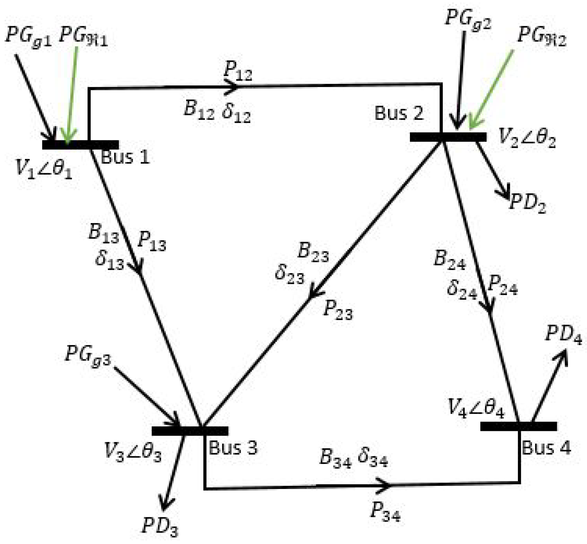
2. Transmission Network Expansion Problem Formulation

2.1. AC TNEP Problem Formulation

The formulation of AC TNEP takes into account the exact power flow equations. The description of the problem entails the incorporation of the real and reactive components of the fossil fuel and the renewable energy generations, voltage magnitude and phase information at each bus for a particular load scenario with regards to the voltage level of each generator, the line conductance, the line susceptance, the phase angle of the line and the real and reactive components of the available loads.

The active and reactive AC power flows in each node of the transmission system are best obtained by searching for the feasible solution to a set of nonlinear nodal balance equations [26].

The available generator capacities are assumed to be constant in the steady state, hence, the unit commitment problem is not considered in the model.

2.2. DC TNEP Problem Formulation

The advantage of the AC grid system has always been that it is more convenient to step-up and step-down the voltage levels using power transformers across the grid system. However, the DC system requires several power converters, which attract extra losses in the system [27].

However, the DC transmission system is gaining more popularity than the AC system because of economical feasibility considerations, the absence of a phase matching problem, the non-skin effect and high power delivery at longer distances [28,29,30].

Hence, this paper considers a DC TNEP model that incorporates the active power flows as the only valuable/tradable commodity in the grid system.

The formulation of the DC TNEP takes into account the linearised version of AC TNEP with some key assumptions, as follows:

• The bus voltage magnitudes must be set to 1.0 p.u. (assuming a uniform bus voltage level for all buses);
• The phase angle difference of the bus voltage is so small that $sin{\delta }_k\approx {\delta }_k$;
• The algebraic sum of the branch flow has to be zero ($P_k^{+}+P_k^{-}=0$);
• The reactive power flow has to be zero;
• The reactive generation has to be zero.

Considering the above assumptions, the active power flow per branch in the DC power network may be simplified as shown in ((1) and (2)).

$$P_k^{+}+B_k{\delta }_k=0$$

(1)

$$P_k^{-}-B_k{\delta }_k=0$$

(2)

where $P_k^{+}$ and $P_k^{-}$ are the respective power flows in and out of the transmission line k. ${\delta }_k$ is the phase angle of transmission line k, and $B_k$ is the susceptance of transmission line k.

The DC power flow nodal balance equation is as follows:

$$\sum _{g=1}^G{P}_g+\sum _{\Re =1}^R{P}_{\Re }-\sum _{k=1}^K{P}_k^{+}+\sum _{k=1}^K{P}_k^{-}=\sum _{d=1}^D{P}_d$$

(3)

where $P_g$ is the fossil fuel generation capacity of generator g. $P_{\Re }$ is the renewable generation capacity of renewable source ℜ, and $P_d$ is the energy demand at load bus d.

Hence, the complete linearised DC TNEP problem is formulated as shown below.

$$Min.\sum _{k=1}^K\sum _{\tau =1}^T\frac{c_z{z}_{k\tau }}{{(1+\lambda )}^{\tau }}+\sum _{g=1}^G\sum _{\tau =1}^T\frac{c_g{P}_{g\tau }}{{(1+\lambda )}^{\tau }}+\sum _{\Re =1}^R\sum _{\tau =1}^T\frac{c_{\Re }{P}_{\Re \tau }}{{(1+\lambda )}^{\tau }}$$

(4)

$$\mathrm{Subject}\mathrm{to}:$$

$$\sum _{g=1}^G{P}_g+\sum _{\Re =1}^R{P}_{\Re }-\sum _{k=1}^K{P}_k^{+}+\sum _{k=1}^K{P}_k^{-}=\sum _{d=1}^D{P}_d$$

(5)

$$P_k^{+}+B_k{\delta }_k=0$$

(6)

$$P_k^{-}-B_k{\delta }_k=0$$

(7)

$$-(1-z_k)M\le (P_k-B_k{\delta }_k)\le M(1-z_k)$$

(8)

$$-P_k^{max}\le P_k\le P_k^{max}$$

(9)

$$-z_k{P}_k^{max}\le P_k\le z_k{P}_k^{max}$$

(10)

$$-{\delta }^{min}\le {\delta }_k\le {\delta }^{max}$$

(11)

$$P_g\le P_g^{max}$$

(12)

$$P_{\Re }\le P_{\Re }^{max}$$

(13)

$$z_k\in [0, 1]$$

(14)

where $z_{k\tau }$, $P_{g\tau }$ and $P_{\Re \tau }$ are the prospective line, fossil fuel generation capacity and the renewable capacity decision variables over the planning period $\tau$, respectively. The fraction, $\frac{1}{{(1+\lambda )}^{\tau }}$ is the discount factor. $c_z$, $c_g$ and $c_{\Re }$ are transmission line investment costs, the costs of fossil fuel generation capacity and the costs of renewable generation capacity over the planning period, respectively. $P_g^{max}$ is the maximum fossil fuel generation capacity at generator bus g, $P_{\Re }^{max}$ is the maximum renewable generation capacity of generator ℜ, $-{\delta }^{min}$ and ${\delta }^{max}$ are the minimum and maximum phase angles of the prospective transmission lines, respectively. M is the disjunctive big-M. The value of M should be large enough to relax the constraint, but it should not be too large, to avoid infeasible solutions [31,32]. The integer variable $z_k\in [0,1]$ returns one if a new line or a new corridor is to be constructed and zero if otherwise.

The DC TNEP model represents only the linear term of the original quadratic model of the AC TNEP and that brings convexity, which allows for faster computation time [33].

2.3. Explicit Expansion of the DC TNEP Model in Matrix Form

The developed model is further represented in the matrix form (represented from (15) to (30), and the summary is shown in

Table 1. The summary of the DC TNEP Matrix Model.

${\mathit{z}}_{\mathit{k}}$	${\mathit{P}}_{\mathit{k}}^{\mathit{e}}$	${\mathit{P}}_{\mathit{k}}^{\mathit{z}}$	${\mathit{\delta }}_{\mathit{k}}^{\mathit{e}}$	${\mathit{\delta }}_{\mathit{k}}^{\mathit{z}}$	$\mathit{\theta }$	${\mathit{P}}_{\mathit{g}}$	${\mathit{P}}_{\mathit{\Re }}$	b
0	$-C_e^t$	$-C_z^t$	0	0	0	$I_g$	$I_{\Re }$	Pd
0	$I_k^e$	0	$-B_k^e$	0	0	0	0	0
0	0	0	0	$-I_k^e$	$C_e$	0	0	0
0	0	0	$-I_k^z$	0	$C_z$	0	0	0
M	$-I_k^z$	0	0	$B_k$	0	0	0	M
M	$I_k^z$	0	0	$-B_k$	0	0	0	M
$-P_z^{max}$	$-I_k^z$	0	0	0	0	0	0	0
$-P_z^{max}$	$I_k^z$	0	0	0	0	0	0	0

where $I_g$ is the identity matrix of the set of fossil fuel generators. $I_{\Re }$ is the identity matrix of the set of renewable energy generators. $I_k^e$ is the identity matrix of the set of existing lines in k right of way. $I_k^z$ is the identity matrix of the set of prospective lines in k right of way. The right hand side of the constraints is denoted as b.

), as follows.

$$Min.\frac{c_z{z}_{k\tau }}{{(1+\lambda )}^{\tau }}+\frac{c_g{P}_{g\tau }}{{(1+\lambda )}^{\tau }}+\frac{c_{\Re }{P}_{\Re \tau }}{{(1+\lambda )}^{\tau }}$$

(15)

$$\mathrm{Subject}\mathrm{to}:$$

$$P_g+P_{\Re }-C_e^t{P}_k^e-C_z^t{P}_k^z=P_d$$

(16)

$$P_k^e-B_k^e{\delta }_k^e=0$$

(17)

$$-{\delta }_k^z+C_z\theta =0$$

(18)

$$-{\delta }_k^e+C_e\theta =0$$

(19)

$$P_k^z-B_k^z{\delta }_k^z+M{z}_k\le M$$

(20)

$$-P_k^z+B_k^z{\delta }_k^z+M{z}_k\le M$$

(21)

$$-z_k{P}_z^{max}-P_k^z\le 0$$

(22)

$$-z_k{P}_z^{max}+P_k^z\le 0$$

(23)

$$-P_e^{max}\le P_k^e\le P_e^{max}$$

(24)

$$-2\pi \le {\delta }_k^e\le 2\pi$$

(25)

$$-2\pi \le {\delta }_k^z\le 2\pi$$

(26)

$$-\pi \le \theta \le \pi$$

(27)

$$P_g\le P_g^{max}$$

(28)

$$P_{\Re }\le P_{\Re }^{max}$$

(29)

$$z_k\in [0, 1]$$

(30)

where $C_e^t$ is the branch–node incidence matrix of the existing lines, $C_z^t$ is the branch–node incidence matrix of the prospective lines, $C_e$ is the node–branch incidence matrix of the existing lines, $C_z$ is the node–branch incidence matrix of the prospective lines, ${\delta }_k^e$ is the existing line k phase angle, ${\delta }_k^z$ is the prospective line k phase angle, $\theta$ is the bus phase angle, $B_k^e$ is the susceptance of the existing transmission line k, $B_k^z$ is the susceptance of the prospective transmission line k, $P_e^{max}$ is the maximum power flow in the existing transmission line k, and $P_z^{max}$ is the maximum power flow in the prospective transmission line k.

2.4. Relaxation of the Negative Variables

In order to carry out the multi-period simulation of the developed model, it is necessary to derive new non-negative variables that can avoid negative variables in terms of the power flow of the lines, line phase angles and the bus phase angles.

The derivation for new non-negative variables may be established by rearranging the respective limits of the mentioned negative variables of the respective constraints of the already developed TNEP model (refer to (15)–(30)), as follows;

$$0\le P_k^z+z_k{P}_z^{max}\le 2z_k{P}_z^{max}$$

(31)

$$0\le P_k^e+P_e^{max}\le 2P_e^{max}$$

(32)

$$0\le {\delta }_k^e+2\pi \le 4\pi$$

(33)

$$0\le {\delta }_k^z+2\pi \le 4\pi$$

(34)

$$0\le \theta +\pi \le 2\pi$$

(35)

Let the new variables for existing and new power flows, line angle and bus angle, respectively, be ${\Psi }_k^e$, ${\Psi }_k^z$, ${\Delta }_k^e$ and $\Theta$.

Hence,

$${\Psi }_k^e=P^e+P_e^{max}$$

$${\Psi }_k^z=P^z+z{P}_z^{max}$$

$${\Delta }_k^e={\delta }_k^e+2\pi$$

$$\Theta =\theta +\pi$$

The reformulations of the problem with respect to the new variables are as follows:

$$Min.\frac{c_z{z}_{\tau }}{{(1+\lambda )}^{\tau }}+\frac{c_g{P}_{g\tau }}{{(1+\lambda )}^{\tau }}+\frac{c_{\Re }{P}_{\Re \tau }}{{(1+\lambda )}^{\tau }}$$

(36)

$$\mathrm{Subject}\mathrm{to}:$$

$$z_k{C}_z^t{P}_z^{max}+P_g+P_{\Re }-C_e^t{\Psi }_k^e-C_z^t{\Psi }_k^z=P_d-C_e^t{P}_e^{max}$$

(37)

$${\Psi }_k^e-B_k^e{\delta }_k^e=P_e^{max}-2\pi B_k^e$$

(38)

$$-{\Delta }_k^e+C_e\Theta =C_e\pi -2\pi$$

(39)

$$-{\Delta }_k^z+C_z\Theta =C_z\pi -2\pi$$

(40)

$$M{z}_k-z_k{P}_z^{max}+{\Psi }_k^z-B_k^z({\Delta }_k^z-2\pi )\le M$$

(41)

$$M{z}_k+z_k{P}_z^{max}-{\Psi }_k^z+B_k^z({\Delta }_k^z-2\pi )\le M$$

(42)

$$0\le {\Psi }_k^z\le 2z_k{P}_z^{max}$$

(43)

$$0\le {\Psi }_k^e\le 2P_e^{max}$$

(44)

$$0\le {\delta }_k^e\le 4\pi$$

(45)

$$0\le {\Delta }_k^z\le 4\pi$$

(46)

$$0\le \Theta \le 2\pi$$

(47)

$$P_g\le P_g^{max}$$

(48)

$$P_{\Re }\le P_{\Re }^{max}$$

(49)

$$z_k\in [0, 1]$$

(50)

From (41) and (42), let $M+P_z^{max}=N_z$ and $M-P_z^{max}=n_z$, respectively.

Equations (41) to (49) are then reformulated as equality constraints by adding slack variables, as follows:

$$z_k{n}_z+{\Psi }_k^z-B_k^z{\Delta }^z+s_0=M-2\pi B_k^z$$

(51)

$$z_k{N}_z-{\Psi }_k^z+B_k^z{\Delta }^z+s_1=M+2\pi B_k^z$$

(52)

$${\Psi }_k^z-2z_k{P}_z^{max}+s_2=0$$

(53)

$${\Psi }_k^e+s_3=2P_e^{max}$$

(54)

$${\Delta }_k^e+s_4=4\pi$$

(55)

$${\Delta }_k^z+s_5=4\pi$$

(56)

$$\Theta +s_6=2\pi$$

(57)

$$P_g+s_7=P_g^{max}$$

(58)

$$P_{\Re }+s_8=P_{\Re }^{max}$$

(59)

3. Results and Discussions of the Test Cases

This section presents the simulation results of the proposed model. The models are being tested with four test cases from the IEEE test systems.

The planning horizon for the period of the increase in energy demand is assumed to be from 2024 to 2045.

The simulations is carried in two scenarios. The first scenario is the simulation of the initial state of the networks’ base year, which aims to obtain the present state of the network, and the second scenario is the simulation of the network with a compound increment demand factor of $\lambda$ per-annum for the 20 year planning horizon, which varies according to the nature of the demands of each network test system.

Hence, the future value, $P_d^h$ of the load at the end of the planning horizon is related to base value $P_d^b$, as follows:

$$P_d^h=P_d^b{(1+\lambda )}^{\tau }$$

(60)

where, the reciprocal of the ${(1+\lambda )}^{\tau }$ expression is the discount factor of the overall demand cost.

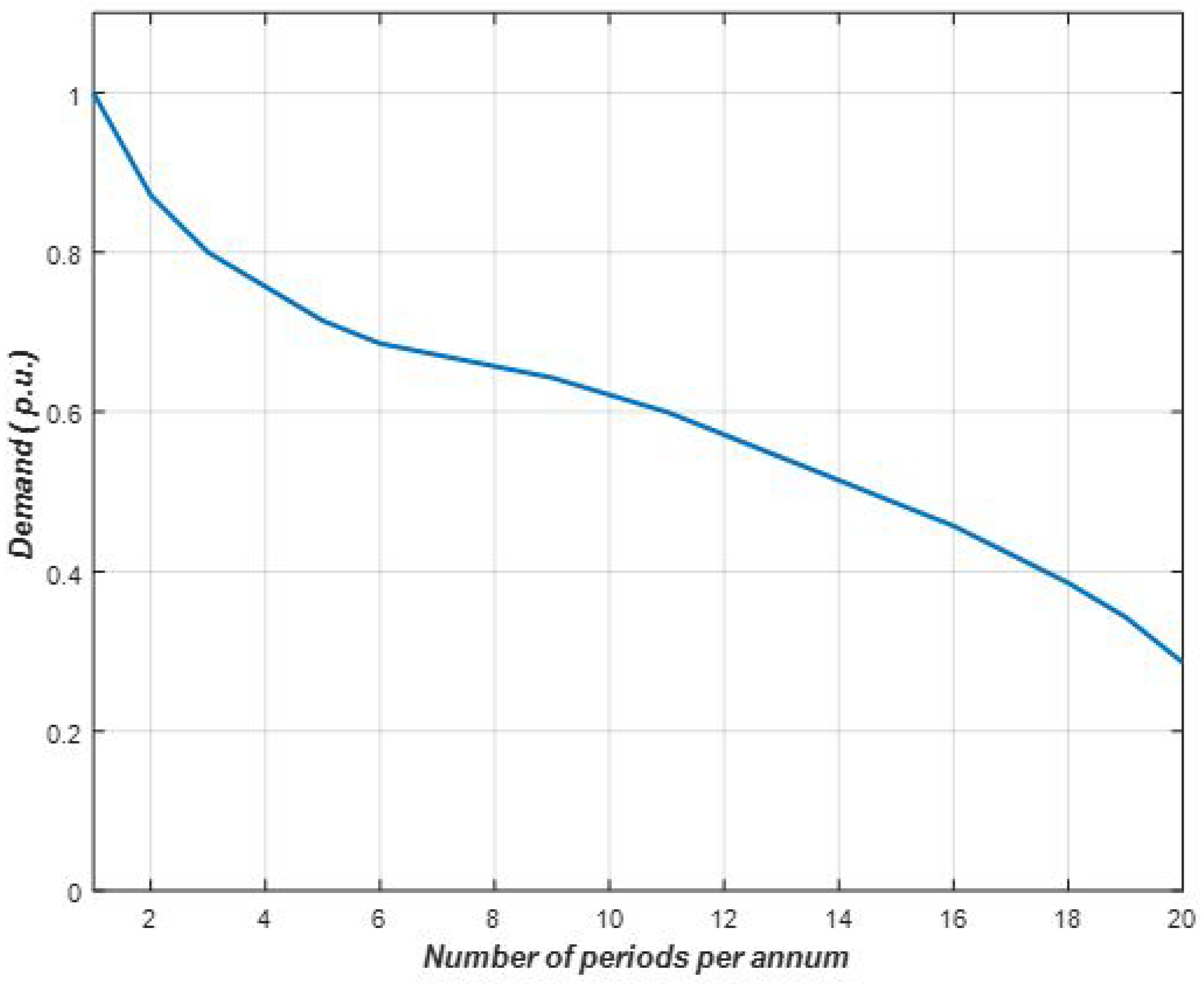
The adopted annual load duration curve (similar to that in [34]) for the study, has an assumed 20 periods per annum with randomised different demand states at different times of the year, as shown in Figure 1.

The obtained results in terms of network reinforcements, new corridors and generations sources represent the recommendation for the long term investment and operation of the power system. However, that may be reviewed annually should there be a new development that may incur additional energy demand that was not included in the previous planning.

Moreover, the approach taken in this paper also provides an additional recommendation in terms of in which particular year (within the 20 year planning period) can the network operators install new line(s), new corridor(s) and/or additional generation capacity to the respective existing power networks. This may be achieved by running incremental period simulations from the base year through the planning horizon and that can aid the power network operators in predicting viable expansion for the optimal operation of the network.

A MATLAB 2022b installed in an Intel(R) Core(TM) i5-2400 CPU @ 3.10 GHz 3.10 GHz 8.00 GB RAM Computer with a 64-bit operating system was used in conducting the simulations. The MATLAB inbuilt solver uses cut generation and a classical linear programming technique to solve the mixed integer linear problem.

The results were recorded and analysed as shown in the next subsections.

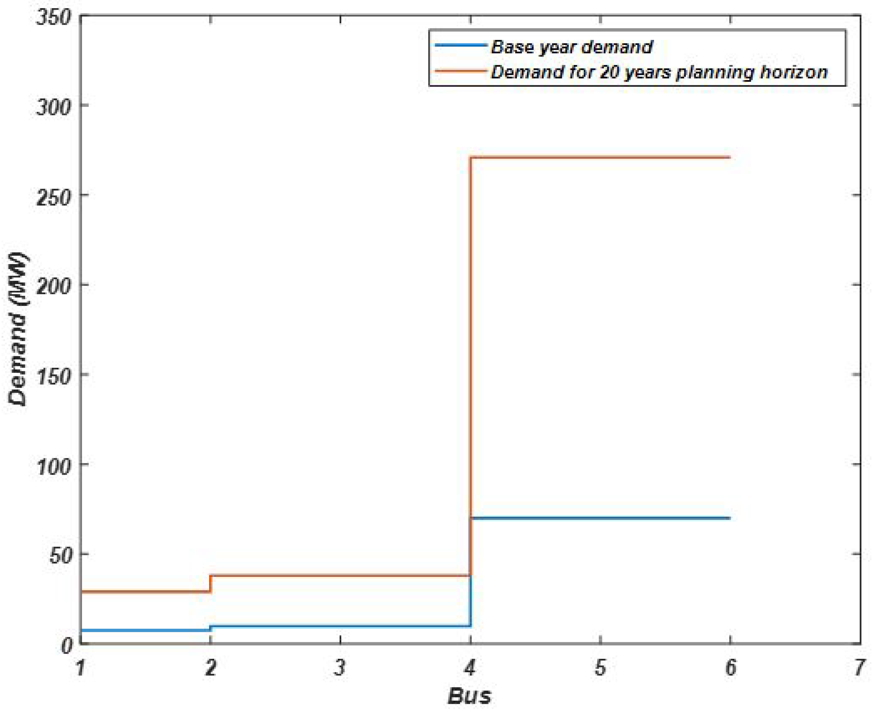
3.1. The IEEE 6-Bus System

The IEEE 6-bus test case system has a total base year energy demand of 241 MW, and the total expected rise in demand over the horizon is based on an annual compounded increase factor of 7%.

The base year demand and the planning horizon demand at each bus are plotted and compared, as shown in Figure 2.

The optimal solution in

Table 2. The optimal results of the line expansions of the IEEE 6-bus system’s expansion over the planning horizon.

fb-tb	OPF (MW)	New Lines	New Corridors
2-5	14.81	1	-
5-4	3.29	-	1

shows that the system needs one new corridor (5-4) and one new line (2-5), along with the rest of the 9 existing lines, to be able to satisfy the expected increase in demand over the planning horizon.

The respective generation capacities at each generator bus are shown in

Table 3. The generation capacity results in the IEEE 6-bus system over the planning horizon.

Bus	${\mathit{P}}_{\mathit{g}}$	${\mathit{P}}_{\mathit{\Re }}$	MGC (MW)
1	155.84	-	200
2	-	101.66	200
3	-	150	150
4	150	-	150
5	180	-	180
6	-	180	180

.

Moreover, the incremental period simulations of the planning horizon further predicted the early useful years of the IEEE 6-bus system’s new line and/or new corridors investments, as shown in

Table 4. The predicted early investment year of the IEEE 6-bus system’s transmission line expansion.

		18th Year	20th Year
fb-tb	OPF (MW)	New Lines	New Corridors
2-5	14.81	1	-
5-4	3.29	-	1

.

Consequently, the incremental period simulations also reveal the incremental steps of the generation capacities, as shown in

Table 5. The predicted years of expected increase in generation capacities (in MW) in the 6-bus system.

	Base Year		3rd Year		5th Year		15th Year		20th Year
Bus	${\mathit{P}}_{\mathit{g}}$	${\mathit{P}}_{\mathbf{\Re }}$	${\mathit{P}}_{\mathit{g}}$	${\mathit{P}}_{\mathbf{\Re }}$	${\mathit{P}}_{\mathit{g}}$	${\mathit{P}}_{\mathbf{\Re }}$	${\mathit{P}}_{\mathit{g}}$	${\mathit{P}}_{\mathbf{\Re }}$	${\mathit{P}}_{\mathit{g}}$	${\mathit{P}}_{\mathbf{\Re }}$
1	-	-	-	-	-	-	24.14	-	155.84	-
2	-	150	-	-	-	-	-	43.2	-	101.66
3	-	-	-	128.82	-	150	-	132.46	-	150
4	-	-	-	-	1.68	-	150	-	150	-
5	87.1	-	150	-	150	-	150	-	150	-
6	-	-	-	2.58	-	51.12	-	180	-	180

, which shows the expected different states of the generators at different periods. Moreover, it may be noticed from Table 5 that renewable energy penetration tends to grow as the time moves upwards due to the quest for global alternative renewable energy sources and the urge to move away from burning fossil fuel due to its negative impacts on global warming.

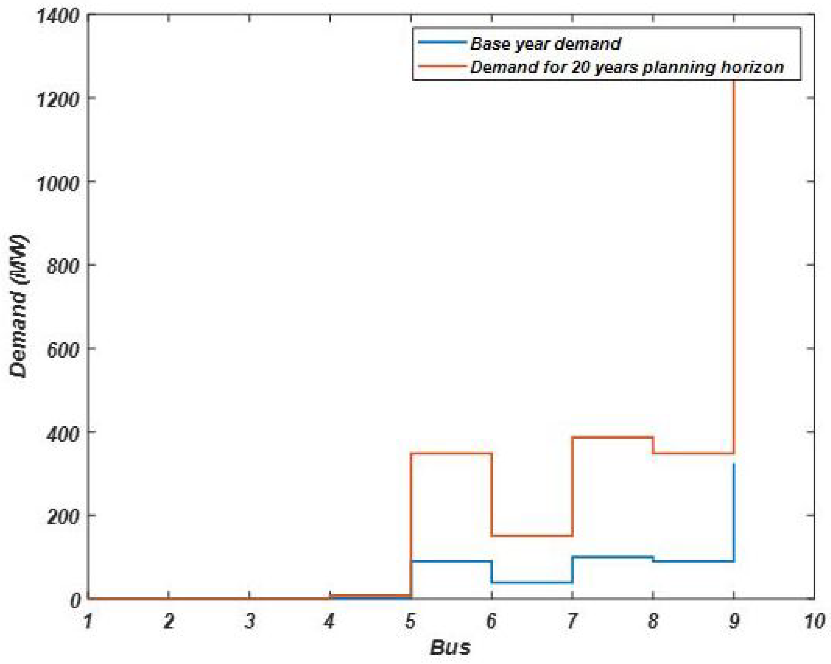
3.2. The IEEE 9-Bus System Test Case Results

The TNEP model was also tested in the IEEE 9-bus system. The system comprises nine existing transmission lines, three fossil fuel generators and three potential renewable energy sources with a total base year demand of 646 MW.

The base year demand and the planning horizon demand for each bus of the network are shown in Figure 3.

With an increment rate of 8% in energy demand per annum, the optimal results in

Table 6. The optimal results of the line expansions of the IEEE 9-bus system’s expansion over the planning period.

fb-tb	OPF (MW)	New Lines	New Corridors
4-9	245.76	1	-
4-9	129.75	1	-
6-7	142.93	1	-
6-1	110.28	-	1

suggest that three new lines and one new corridor should be constructed to satisfy the total energy demand over the planning period. The total generation capacities at each generator bus over the horizon are shown in

Table 7. The generation capacity results in the IEEE 9-bus system over the planning horizon.

Bus No	${\mathit{P}}_{\mathit{g}}$	${\mathit{P}}_{\mathit{\Re }}$	MGC (MW)
4	-	700	700
5	-	300	300
6	659.82	-	700
7	-	270	270
8	300	-	300
9	270	-	270

.

Consequently, the incremental period simulation results further reveal the exact years in which these new lines, new corridors and the generation capacities should be in optimal usable states, as shown in

Table 8. The predicted early investment year of the IEEE 9-bus system’s transmission line expansion.

		13th Year		16th Year		20th Year
fb-tb	OPF (MW)	Lines	Corridors	Lines	Corridors	Lines	Corridors
4-9	194.49	1	-	-	-	-	-
4-9	245.76	-	-	-	-	1	-
6-7	110.04	-	-	1	-	-	-
6-1	110.28	-	-	-	-	-	1

and

Table 9. The predicted years of the expected increase in generation capacities (in MW) in the 9-bus system.

	Base Year		3rd Year		5th Year		10th Year		13th Year
Bus	${\mathit{P}}_{\mathit{g}}$	${\mathit{P}}_{\mathbf{\Re }}$	${\mathit{P}}_{\mathit{g}}$	${\mathit{P}}_{\mathbf{\Re }}$	${\mathit{P}}_{\mathit{g}}$	${\mathit{P}}_{\mathbf{\Re }}$	${\mathit{P}}_{\mathit{g}}$	${\mathit{P}}_{\mathbf{\Re }}$	${\mathit{P}}_{\mathit{g}}$	${\mathit{P}}_{\mathbf{\Re }}$
4	-	-	-	-	-	-	-	-	310.68	-
5	106	-	251.38	-	300	-	300	-	300	-
6	-	-	-	-	-	-	-	130.78	-	106.08
7	270	-	270	-	270	-	270	-	270	-
8	-	-	-	-	-	66.05	-	300	-	300
9	-	270	-	270	-	270	-	270	-	270

.

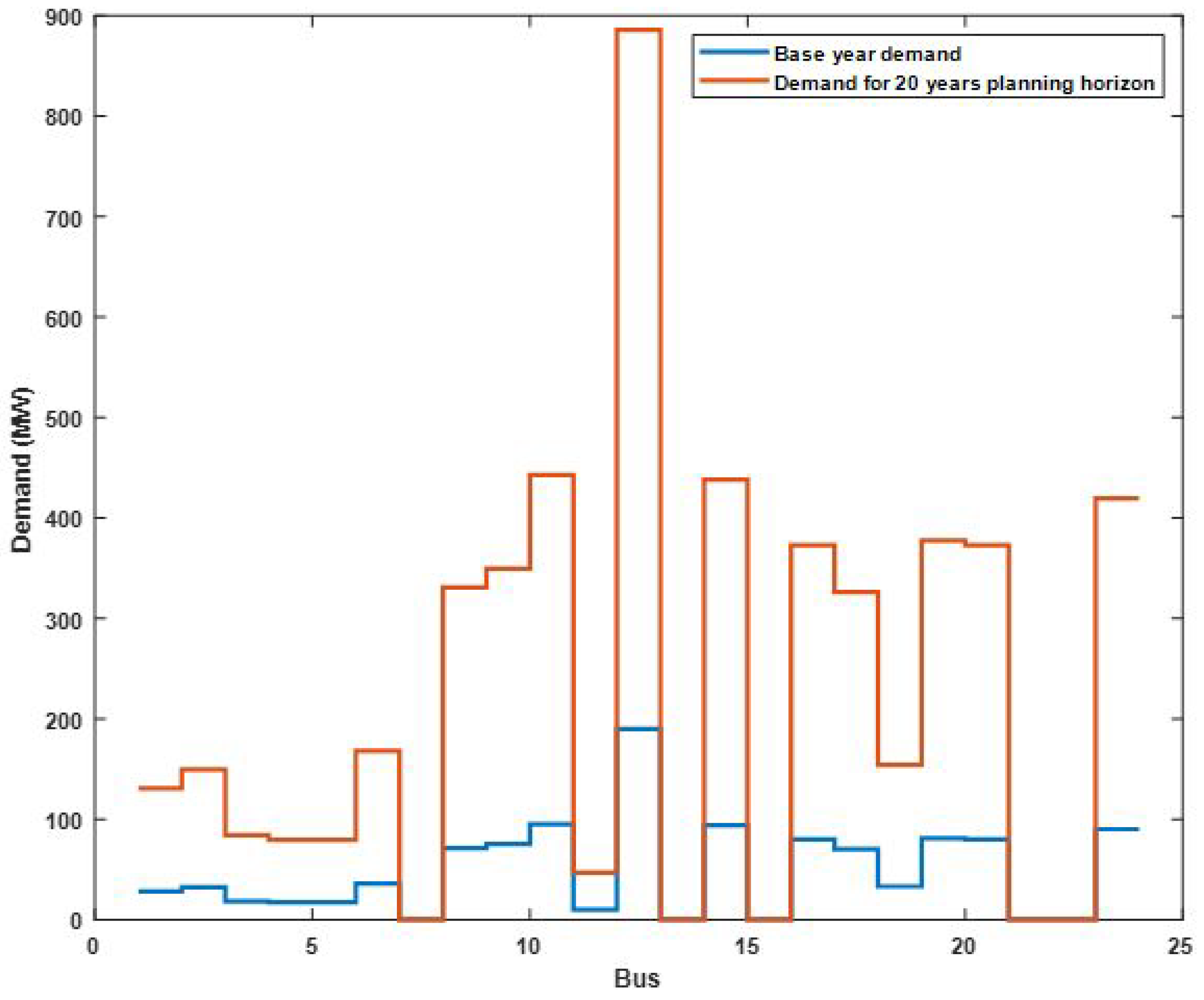
3.3. The IEEE 24-Bus System

The TNEP model was also tested in the IEEE 24-bus system. The system comprises 38 existing transmission lines, 5 fossil fuel generators and 4 potential renewable energy sources with a total base year demand of 1770 MW.

The base year demand and the planning horizon demand for each bus of the 24-bus network are shown in Figure 4.

With an increment rate of 8% in energy demand per annum, the optimal results in

Table 10. The optimal results of line expansions of the IEEE 24-bus system’s expansion over the planning horizon.

fb-tb	OPF (MW)	New Lines	New Corridors
7-8	245.76	2	-
13-12	500	1	-
15-1	175	-	1
16-19	464.16	1	-

suggest that four new lines and one new corridor should be constructed to satisfy the total energy demand over the planning period. The total generation capacities at each generator bus over the horizon are shown in

Table 11. The generation capacity results in the IEEE 24-bus system over the planning horizon.

Bus	${\mathit{P}}_{\mathit{g}}$	MGC (MW)	Bus	${\mathit{P}}_{\mathit{\Re }}$	MGC (MW)
1	24.39	980	16	980	980
2	596.42	1000	21	704.79	1002
7	525	1002	22	929.83	1970
13	1602.3	1970	-	-	-
15	263.06	1112	-	-	-

.

Consequently, the incremental period simulation results further reveal the exact years in which these new lines, new corridors and the generation capacities should be in optimal usable states, as shown in

Table 12. The predicted early investment year of the IEEE 24-bus system’s transmission line expansion.

		5th Year		14th Year		16th Year		20th Year
fb-tb	OPF (MW)	Lines	Cors	Lines	Cors	Lines	Cors	Lines	Cors
15-1	175	-	1	-	-	-	-	-	-
7-8	175	-	-	2	-	-	-	-	-
13-12	500	-	-	-	-	1	-	-	-
16-19	406.41	-	-	-	-	1	-	1	-

and

Table 13. The predicted years of expected increase in generation capacities (in MW) in the 24 bus system.

	Base Year		5th Year		10th Year		14th Year		20th Year
Bus	${\mathit{P}}_{\mathit{g}}$	${\mathit{P}}_{\mathbf{\Re }}$	${\mathit{P}}_{\mathit{g}}$	${\mathit{P}}_{\mathbf{\Re }}$	${\mathit{P}}_{\mathit{g}}$	${\mathit{P}}_{\mathbf{\Re }}$	${\mathit{P}}_{\mathit{g}}$	${\mathit{P}}_{\mathbf{\Re }}$	${\mathit{P}}_{\mathit{g}}$	${\mathit{P}}_{\mathbf{\Re }}$
1	-	-	20.04	-	-	-	-	-	24.39	-
2	-	-	-	-	95.716	-	479.67	-	596.42	-
7	-	-	175	-	175	-	350	-	525	-
13	336.48	-	533.13	-	1131.2	-	1031.2	-	1602.3
15	870.52	-	1045.30	-	1112	-	1112	-	263.06	-
16	-	-	-	-	-	68.17	-	516.38	-	980
21	-	-	-	-	-	-	-	-	-	704.79
22	-	-	-	-	-	23.78	-	55.965	-	929.83

, respectively. It may also be noticed (from Table 13) that renewable energy penetration occurred on the 10th year through buses 16 and 22.

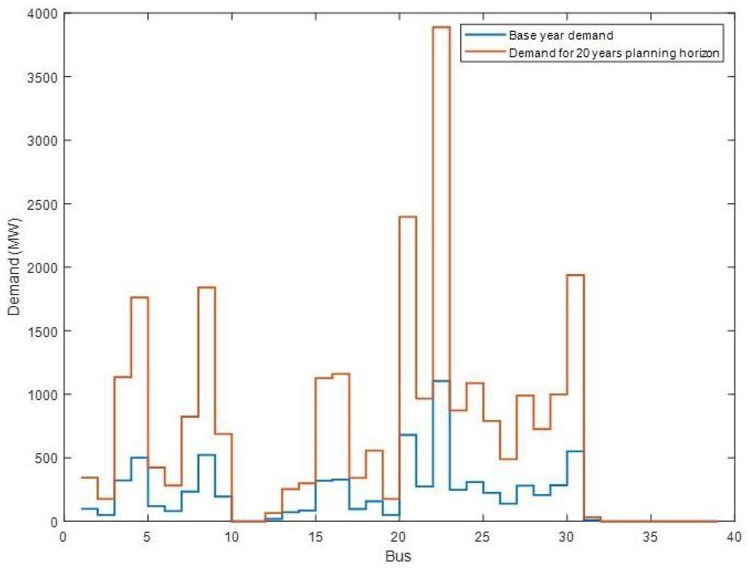
3.4. The IEEE 39-Bus System

The 39-bus system from the IEEE test case systems has a total base year energy demand of 7556.73 MW located across 29 different load buses. The system also comprises 46 existing transmission lines, 9 fossil fuel generators and 9 potential renewable energy sources.

The base year demand and the planning horizon demand for each bus of the 39-bus network are shown in Figure 5.

With the demand increment rate of 6.5% per annum, the optimal results in

Table 14. The optimal results of line expansions of the IEEE 39-bus system’s expansion over the planning period.

fb-tb	OPF (MW)	New Lines	New Corridors	fb-tb	OPF (MW)	New Lines
3-18	500	1	-	33-19	900	1
25-4	500	-	1	35-22	712.94	1
6-7	843.53	1	-	36-23	687	2
7-16	480	-	1	23-22	545.31	2
11-6	480	1	-	20-34	900	1
39-9	738.28	-	1	27-17	566.18	2
17-16	600	2	-	16-21	597.93	2
19-16	513.87	1	-

suggest that 17 new lines and 3 new corridors should be constructed to satisfy the total energy demand over the planning period. The total generation capacities at each generator bus over the horizon are shown in

Table 15. The generation capacity results in the IEEE 39-bus system over the planning horizon.

Bus	${\mathit{P}}_{\mathit{g}}$	MGC (MW)	Bus	${\mathit{P}}_{\mathit{\Re }}$	MGC (MW)
30	2557.9	3120	3	1793.5	2175
33	1800	1956	4	1956	1956
34	1524	1524	10	70.57	1524
35	2061	2061	11	1577.9	2061
36	1425.9	1740	24	1740	1740
37	900	1692	26	1692	1692
38	1200	2595	27	2121.5	2595
39	2098.5	3300	31	1832.4	2033.61

.

Consequently, the incremental period simulation results further reveal the exact years in which these new lines, new corridors and the generation capacities should be in optimal usable states, as shown in

Table 16. The predicted in-use year of the IEEE 39-bus system’s transmission line extensions.

		8th Year	12th Year		16th Year	20th Year
fb-tb	OPF (MW)	Lines	Lines	Cors	Lines	Lines	Cors
16-21	390.29	1	-	-	-	-	-
35-22	762	-	1	-	-	-	-
7-16	480	-	-	1	-	-	-
3-18	500	-	-	-	1	-	-
34-20	849.74	-	-	-	1	-	-
17-16	599.08	-	-	-	1	-	-
27-17	448.30	-	-	-	1	-	-
23-22	600	-	-	-	1	-	-
36-23	809.41	-	-	-	1	-	-
6-7	843.53	-	-	-	-	1	-
11-6	480	-	-	-	-	1	-
17-16	600	-	-	-	-	1	-
19-16	513.87	-	-	-	-	1	-
25-4	500	-	-	-	-	-	1
39-9	738.28	-	-	-	-	-	1
16-21	597.93	-	-	-	-	1	-
27-17	566.18	-	-	-	-	1	-
33-19	900	-	-	-	-	1	-
23-22	545.31	-	-	-	-	1	-
36-23	687	-	-	-	-	1	-

and

Table 17. The predicted years of expected change in generation capacities (in MW) in the 39-bus system.

	Base Year		8th Year		12th Year		16th Year		20th Year
Bus	${\mathit{P}}_{\mathit{g}}$	${\mathit{P}}_{\mathbf{\Re }}$	${\mathit{P}}_{\mathit{g}}$	${\mathit{P}}_{\mathbf{\Re }}$	${\mathit{P}}_{\mathit{g}}$	${\mathit{P}}_{\mathbf{\Re }}$	${\mathit{P}}_{\mathit{g}}$	${\mathit{P}}_{\mathbf{\Re }}$	${\mathit{P}}_{\mathit{g}}$	${\mathit{P}}_{\mathbf{\Re }}$
3	-	1075.3	-	2032.9	-	1221.4	-	1603.1	-	1793.5
4	-	-	-	726.67	-	1956	-	1956	-	1956
10	-	-	-	-	-	1027.6	-	1109.8	-	70.57
11	-	550.72	-	-	-	-	-		-	1577.9
24	-	893.21	-	1328.7	-	1460.7	-	1704.3	-	1740
26	-	-	-	-	-	-	-	-	-	1692
27	-	-	-	355.25	-	654.06	-	1066.3	-	2121.5
28	-	434.33	-	718.82	-	924.74	-	1005.6	-	-
30	-	-	290.86	-	271	-	1930.4	-	2557.9	-
31	-	383.79	-	1815.2	-	916.05	-	1270.4	-	1832.4
32	-	-	-	-	-	-	-	-	-	-
33	430	-	900	-	900	-	900	-	1800	-
34	900	-	900	-	900	-	1699.5	-	1524	-
35	577.37	-	900	-	1524	-	1524	-	2061	-
36	862.89	-	791.65	-	900	-	1618.8	-	1425.9	-
37	249.1	-	546.28	-	734.53	-	900	-	900	-
38	1200	-	1200	-	1200	-	1200	-	1200	-
39	-	-	-	-	1499	-	1209.7	-	2098.5	-

.

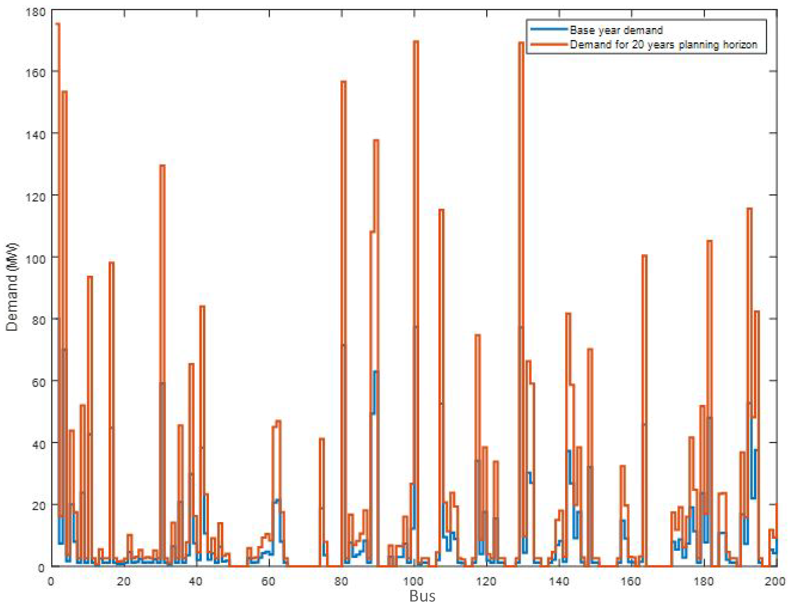
3.5. The IEEE 200-Bus System

For the purpose of reassuring robustness of the model in handling a large network system, the IEEE 200-bus system was adopted. The system comprises 246 existing transmission lines, 24 fossil fuel generators and 24 potential renewable energy sources with a total base year demand of 1802.5 MW.

The base year demand and the planning horizon demand for each bus of the 200-bus network are shown in Figure 6.

Due to the demand pattern across the 200 buses, the compounded annual demand increment rate is chosen to be 4%.

The optimal results in

Table 18. The optimal results of line expansions of the IEEE 200-bus system’s expansion over the planning period.

fb-tb	OPF (MW)	New Lines	New Corridors	fb-tb	OPF (MW)	New Lines
11-15	16.67	1	-	90-89	8.6	1
11-113	100	-	1	38-36	63.26	1
116-15	14.78	-	1	29-30	64.74	1
22-123	22.91	-	1	158-22	16.67	1
154-34	77.74	-	1	76-75	24.3	1
134-137	24.80	-	1	107-129	10.61	1
177-31	83.16	1	-	112-113	23.80	1
31-192	74.23	1	-	114-112	11.05	1
127-158	23.84	-	1	67-66	30	1
140-129	47.46	-	1	113-192	22.09	1
136-38	95.92	-	1	116-117	90.75	1
136-83	29.94	-	1	123-124	271.93	1
77-75	7.4	1	-	126-123	148.72	1
79-75	39.60	1	-	127-123	170	1
149-114	2.17	-	1	93-191	18.69	1
133-128	58.44	1	-	134-140	50.36	1
147-146	130.60	1	-	146-177	97.55	1
151-149	10.34	1	-	164-163	58.1	1
167-163	39.60	1	-	168-163	39.60	1
183-181	39.60	1	-	196-195	87.70	1

recommend 30 new lines and 10 new corridors to be constructed to satisfy the total energy demand over the planning period. The total generation capacities in each generator bus over the horizon are shown in

Table 19. The generation capacity results in the IEEE 200-bus system.

Bus	${\mathit{P}}_{\mathit{g}}$	MGC (MW)	Bus	${\mathit{P}}_{\mathit{\Re }}$	MGC (MW)
49	19.93	19.93	65	19.93	19.93
50	19.93	19.93	104	19.93	19.93
51	19.93	19.93	105	19.93	19.93
52	19.93	19.93	114	19.93	19.93
53	35.3	39.91	115	39.91	39.91
67	60	380.6	147	261.2	380.6
68	20.10	20.68	151	20.68	20.68
69	70.50	122.85	152	100	122.85
70	70.50	122.85	153	100	122.85
71	68	122.85	154	122.85	122.85
72	68	122.85	155	122.85	122.85
73	65	122.85	161	122.85	122.85
76	48.6	122.85	164	116.2	122.85
77	14.8	17.6	165	17.6	17.6
78	10.56	10.56	166	10.56	10.56
70	79.2	79.2	167	79.2	79.2
90	17.2	79.2	168	79.2	79.2
91	14.08	14.08	169	14.08	14.08
92	22	22	170	22	22
125	79.2	79.2	182	27.68	27.68
126	297.44	297.44	183	79.2	79.2
127	363.84	681.12	189	297.44	297.44
135	6.16	6.16	196	175.4	681.12
136	587.4	587.4	197	6.16	6.16

.

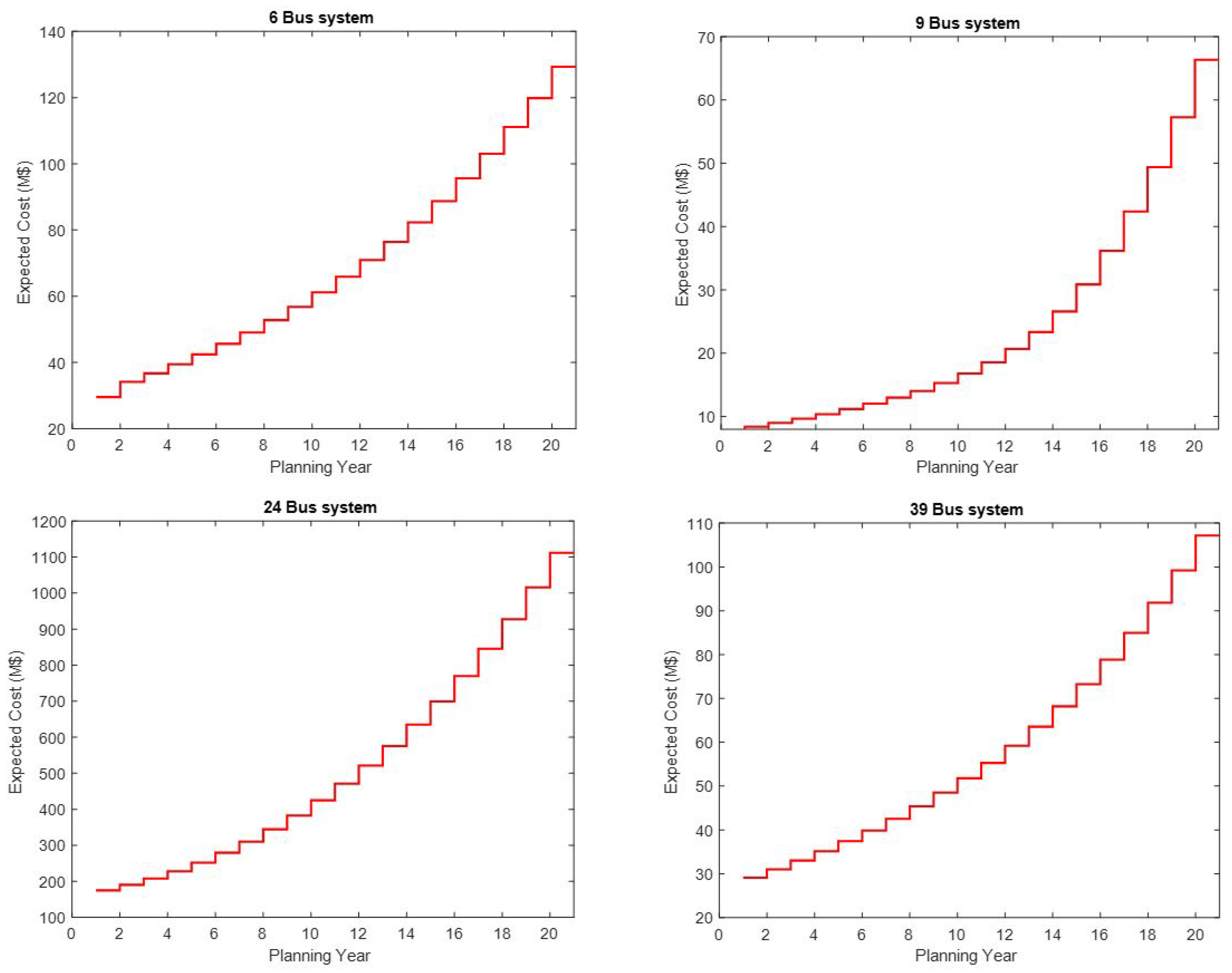
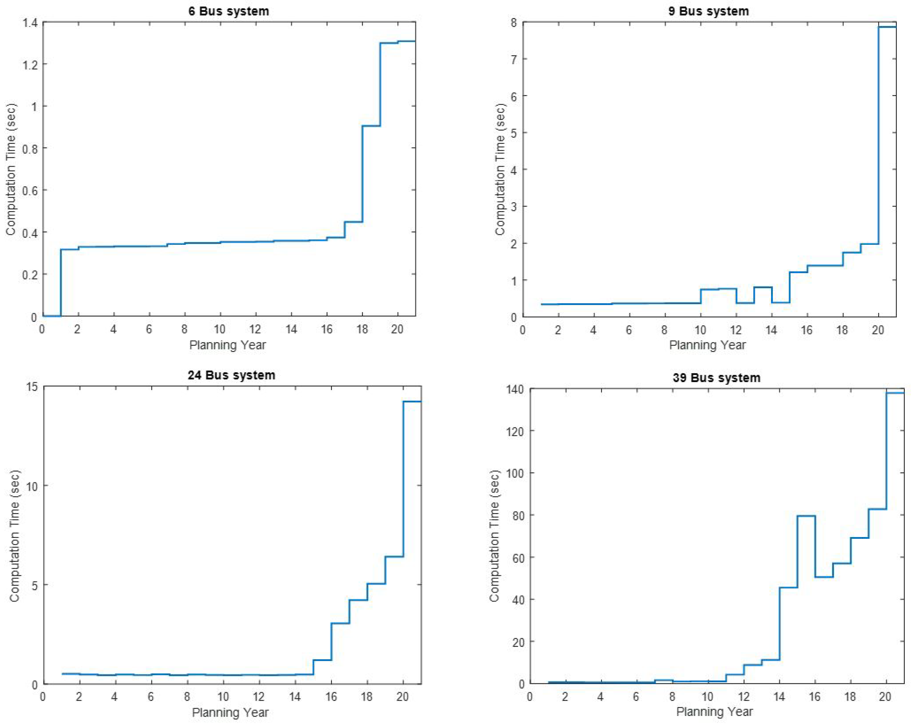
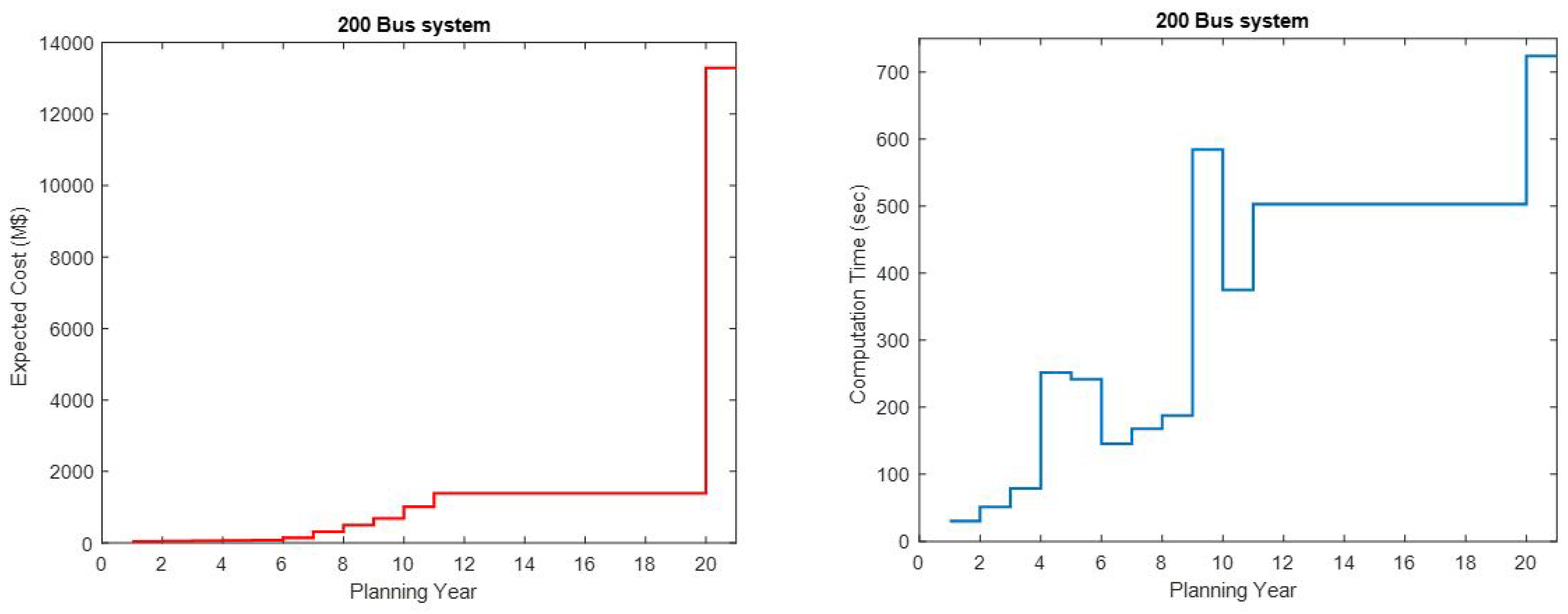
The planning horizon total costs and the computation times for the different network sizes are shown in

Table 20. The planning horizon total costs and the computation times for the different network sizes.

Network Size	Cost (M USD)	Computation Time (s)
6-bus system	67.5	1.34
9-bus system	132	7.9
24-bus system	1108	14.1
39-bus system	2208	139
200-bus system	13,255	715

. The graph of the computation times for the different tested network sizes is shown in Figure A2, and the optimal total costs of the network test systems obtained during the course of the simulation are shown in Figure A3; whereas Figure A4 shows the computation time and total cost curves for the 200-bus system.

It can be noticed in Figure A2 and Figure A4 that the computation times fall within the acceptable finite time ranges for the respective test systems.

Moreover, it was observed that a higher number of candidate integer variables increases the computation times and can lead to premature termination without reaching the optimal solution.

4. Conclusions

Power transmission network modelling plays a crucial role in the expansion planning procedure. It is of high importance to understand the fundamental behaviour of the system, which will allow the facilitation of the formulation of an appropriate mathematical optimisation model and also aid for a better decision in the planning process.

The long term planning is normally carried out in the first year of the planning horizon, and the obtained results, in terms of new transmission lines, new corridors, fossil fuel generators and renewable sources, represent the recommendation for the long term investment and operation of the power system. However, this can be reviewed annually should there be a new development that can incur additional energy demand that was not included in the previous planning.

In this paper, TNEP was tackled as a DC-TNEP problem that minimises the investment cost of adding new circuits, fossil fuel generators’ operation costs and the costs of renewable energy penetrations while satisfying the increase in demand and other constraints. It is formulated as a mixed integer linear programming (MILP) model. It was tested on IEEE 6-, 9-, 24-, 39- and 200-bus test systems within acceptable finite computation times, and the subsequent considerations are reported in Table 20.

The discussion of the obtained results is relevant and has highlighted the value of the proposed approach.

The adopted annual load duration curve has an assumed 20 periods per annum with randomised different demand states at different times of the year, which resulted in a multi-period of a 20 year TNEP horizon. The idea is to establish the information regarding the annual evolution of the generator capacities and the corresponding available demands.

The major finding in this work shows in which particular year (within the 20 years of the planning period) can the network operators install new line(s), new corridor(s) and/or additional generation capacity to the respective existing power networks. This was achieved by running incremental period simulations from the base year through the planning horizon.

Moreover, other aspects of the findings, which are obvious inference, show that the increments in demand in different test systems in use do not follow similar patterns. This is because each of the test systems has different network characteristics in terms of the network parameters, generation and demand patterns.

In other words, they do not maintain a unified pattern of changes. For instance, Table 5 and Table 9 show that penetrations of renewable energy generation first occur at the base year of the planning horizon in -6 and 9-bus test systems. However, Table 13 shows that these penetrations can only start at the 10th year of the planning horizon in a 24-bus test system.

Hence, due to the fact that different network sizes are being used for the test cases, the stages of their changes in generation capacities and demands are not uniform.

Finally, the aim of this paper is to make recommendations for power transmission utilities, the optimal method of long term power transmission network expansion planning, with the major goal of expanding the existing network by predicting possible new renewable and fossil fuel generating points and new transmission lines/corridors to meet the future energy demand, without violating the system’s reliability and efficiency.

In addition, the idea of this research article is highly crucial for modern day DC power networks, and hence, it can be applied in practice by first, performing an optimal power flow (OPF) analysis in the power network to obtain the present status of the network and to see where there are bottlenecks that attract network expansion. The simulation of the developed model in terms of the minimisation of the additional network construction and operational costs while satisfying the demand increase imposed by technical and economic conditions over the planning horizon should provide additional information regarding possible new generation points and exploring better transmission line corridors that can yield an optimal expansion over the planning horizon while considering all the respective constraints.

References

1. Zhang, X.; Conejo, A.J. Candidate line selection for transmission expansion planning considering long-and short-term uncertainty. Int. J. Electr. Power Energy Syst. 2018, 100, 320–330. [Google Scholar] [CrossRef]
2. Ude, N.G.; Yskandar, H.; Graham, R.C. A comprehensive state-of-the-art survey on the transmission network expansion planning optimization algorithms. IEEE Access 2019, 7, 123158–123181. [Google Scholar]
3. Morquecho, E.G.; Torres, S.P.; Astudillo-Salinas, F.; Castro, C.A.; Ergun, H.; Van Hertem, D. Security constrained AC dynamic transmission expansion planning considering reactive power requirements. Electr. Power Syst. Res. 2023, 221, 109419. [Google Scholar] [CrossRef]
4. Mahdavi, M.; Javadi, M.S.; Catalão, J.P. Integrated generation-transmission expansion planning considering power system reliability and optimal maintenance activities. Int. J. Electr. Power Energy Syst. 2023, 145, 108688. [Google Scholar] [CrossRef]
5. Khodaei, A.; Shahidehpour, M.; Kamalinia, S. Transmission switching in expansion planning. IEEE Trans. Power Syst. 2010, 25, 1722–1733. [Google Scholar] [CrossRef]
6. Shaheen, A.M.; El-Sehiemy, R.A. Application of multi-verse optimizer for transmission network expansion planning in power systems. In Proceedings of the 2019 International Conference on Innovative Trends in Computer Engineering (ITCE), Aswan, Egypt, 2–4 February 2019; IEEE: Piscataway, NJ, USA, 2019; pp. 371–376. [Google Scholar]
7. Gan, W.; Ai, X.; Fang, J.; Yan, M.; Yao, W.; Zuo, W.; Wen, J. Security constrained co-planning of transmission expansion and energy storage. Appl. Energy 2019, 239, 383–394. [Google Scholar] [CrossRef]
8. Hemmati, R.; Hooshmand, R.A.; Khodabakhshian, A. State-of-the-art of transmission expansion planning: Comprehensive review. Renew. Sustain. Energy Rev. 2013, 23, 312–319. [Google Scholar] [CrossRef]
9. Ramos, A.; Lumbreras, S. How to solve the transmission expansion planning problem faster: Acceleration techniques applied to Benders’ decomposition. IET Gener. Transm. Distrib. 2016, 10, 2351–2359. [Google Scholar]
10. Lumbreras, S.; Ramos, A. Transmission expansion planning using an efficient version of Benders’ decomposition. A case study. In Proceedings of the PowerTech (POWERTECH), 2013 IEEE Grenoble, Grenoble, France, 16–20 June 2013; IEEE: Piscataway, NJ, USA, 2013; pp. 1–7. [Google Scholar]
11. Zambrano, C.; Arango-Aramburo, S.; Olaya, Y. Dynamics of power-transmission capacity expansion under regulated remuneration. Int. J. Electr. Power Energy Syst. 2019, 104, 924–932. [Google Scholar] [CrossRef]
12. Zhang, H.; Heydt, G.T.; Vittal, V.; Quintero, J. An improved network model for transmission expansion planning considering reactive power and network losses. IEEE Trans. Power Syst. 2013, 28, 3471–3479. [Google Scholar] [CrossRef]
13. Hamam, Y.; Renders, M.; Trecat, J. Partitioning algorithm for the solution of long-term power-plant mix problems. Proc. Inst. Electr. Eng. 1979, 126, 837–839. [Google Scholar]
14. Wang, Y.; Zhou, X.; Shi, Y.; Zheng, Z.; Zeng, Q.; Chen, L.; Xiang, B.; Huang, R. Transmission Network Expansion Planning Considering Wind Power and Load Uncertainties Based on Multi-Agent DDQN. Energies 2021, 14, 6073. [Google Scholar] [CrossRef]
15. Davoodi, A.; Abbasi, A.R.; Nejatian, S. Multi-objective dynamic generation and transmission expansion planning considering capacitor bank allocation and demand response program constrained to flexible-securable clean energy. Sustain. Energy Technol. Assess. 2021, 47, 101469. [Google Scholar] [CrossRef]
16. Giannelos, S.; Jain, A.; Borozan, S.; Falugi, P.; Moreira, A.; Bhakar, R.; Mathur, J.; Strbac, G. Long-Term Expansion Planning of the Transmission Network in India under Multi-Dimensional Uncertainty. Energies 2021, 14, 7813. [Google Scholar] [CrossRef]
17. Li, C.; Conejo, A.J.; Liu, P.; Omell, B.P.; Siirola, J.D.; Grossmann, I.E. Mixed-integer linear programming models and algorithms for generation and transmission expansion planning of power systems. Eur. J. Oper. Res. 2022, 297, 1071–1082. [Google Scholar] [CrossRef]
18. Lara, C.L.; Mallapragada, D.S.; Papageorgiou, D.J.; Venkatesh, A.; Grossmann, I.E. Deterministic electric power infrastructure planning: Mixed-integer programming model and nested decomposition algorithm. Eur. J. Oper. Res. 2018, 271, 1037–1054. [Google Scholar] [CrossRef]
19. Pache, C.; Maeght, J.; Seguinot, B.; Zani, A.; Lumbreras, S.; Ramos, A.; Agapoff, S.; Warland, L.; Rouco, L.; Panciatici, P. New Methodology for Long-Term Transmission Grid Planning–General Description. 2018. [Google Scholar]
20. Davoodi, A.; Abbasi, A.R.; Nejatian, S. Multi-objective techno-economic generation expansion planning to increase the penetration of distributed generation resources based on demand response algorithms. Int. J. Electr. Power Energy Syst. 2022, 138, 107923. [Google Scholar] [CrossRef]
21. Le Roux, P.; Ngwenyama, M.; Aphane, T. 14-Bus IEEE Electrical Network Compensated for Optimum Voltage Enhancement using FACTS Technologies. In Proceedings of the 2022 3rd International Conference for Emerging Technology (INCET), Belgaum, India, 27–29 May 2022; IEEE: Piscataway, NJ, USA, 2022; pp. 1–7. [Google Scholar]
22. Toloo, M.; Taghizadeh-Yazdi, M.; Mohammadi-Balani, A. Multi-objective centralization-decentralization trade-off analysis for multi-source renewable electricity generation expansion planning: A case study of Iran. Comput. Ind. Eng. 2022, 164, 107870. [Google Scholar] [CrossRef]
23. Rothlauf, F. Design of Modern Heuristics: Principles and Application; Springer: Berlin/Heidelberg, Germany, 2011; Volume 8. [Google Scholar]
24. Keokhoungning, T.; Premrudeepreechacharn, S.; Wongsinlatam, W.; Namvong, A.; Remsungnen, T.; Mueanrit, N.; Sorn-in, K.; Kravenkit, S.; Siritaratiwat, A.; Srichan, C.; et al. Transmission Network Expansion Planning with High-Penetration Solar Energy Using Particle Swarm Optimization in Lao PDR toward 2030. Energies 2022, 15, 8359. [Google Scholar] [CrossRef]
25. Nnachi, G.U.; Hamam, Y.; Richards, C.G. Appraising the Optimal Power Flow and Generation Capacity in Existing Power Grid Topology with Increase in Energy Demand. Energies 2022, 15, 2522. [Google Scholar] [CrossRef]
26. Vellingiri, M.; Rawa, M.; Alghamdi, S.; Alhussainy, A.A.; Ali, Z.M.; Turky, R.A.; Refaat, M.M.; Aleem, S.H.A. Maximum hosting capacity estimation for renewables in power grids considering energy storage and transmission lines expansion using hybrid sine cosine artificial rabbits algorithm. Ain Shams Eng. J. 2023, 14, 102092. [Google Scholar] [CrossRef]
27. Rahman, M.; Ashraf, I.; Alsharari, H.D. HVDC system for national and cross border grid interconnections in Saudi Arabia. IOSR J. Eng. 2012, 2, 529–537. [Google Scholar] [CrossRef]
28. Kamalapur, G.; Sheelavant, V.; Pujar, A.; Baksi, S.; Patil, A. HVDC transmission in India. IEEE Potentials 2014, 33, 22–27. [Google Scholar] [CrossRef]
29. Bhattacharjee, S.; Nandi, C.; Reang, S. Intelligent energy management controller for hybrid system. In Proceedings of the 2018 3rd International Conference for Convergence in Technology (I2CT), Pune, India, 6–8 April 2018; IEEE: Piscataway, NJ, USA, 2018; pp. 1–7. [Google Scholar]
30. Mohamed, A.T.; El-Morshedy, A.; Tag-Eldin, E.; Emam, A.; Samy, M.M. Increasing Transmitted Power With Cost Mitigation via Modified EHV Power Lines in Egyptian Grid. IEEE Access 2023, 11, 21554–21561. [Google Scholar] [CrossRef]
31. Balas, E. Disjunctive programming. Ann. Discret. Math. 1979, 5, 3–51. [Google Scholar]
32. Balas, E. Disjunctive Programming; Springer: Berlin/Heidelberg, Germany, 2018. [Google Scholar]
33. Overbye, T.J.; Cheng, X.; Sun, Y. A comparison of the AC and DC power flow models for LMP calculations. In Proceedings of the 37th Annual Hawaii International Conference on System Sciences, Big Island, HI, USA, 5–8 January 2004; IEEE: Piscataway, NJ, USA, 2004; p. 9. [Google Scholar]
34. Soltani, S.; Soltani, N.; Haghifam, M.R.; Jahromi, M.Z. A Feasibility Study of Wind Farm Installation Based on Reliability Assessment in Kish Island. In Proceedings of the 28th International Power System Conference, Tehran, Iran, 4–6 November 2013. [Google Scholar]
Figure 1. The adopted annual load duration curve [34].
Computation 11 00179 g001
Figure 2. The 6-bus system’s base year versus the planning horizon demand.
Computation 11 00179 g002
Figure 3. The 9-bus system’s base demand versus the increase in demand over the planning period.
Computation 11 00179 g003
Figure 4. The 24-bus system’s base year versus planning horizon demands.
Computation 11 00179 g004
Figure 5. The 39-bus system’s base year versus planning horizon demands.
Computation 11 00179 g005
Figure 6. The 200-bus system’s base year versus planning horizon demands.
Computation 11 00179 g006