Filter Pruning with Convolutional Approximation Small Model Framework

Abstract

Convolutional neural networks (CNNs) are extensively utilized in computer vision; however, they pose challenges in terms of computational time and storage requirements. To address this issue, one well-known approach is filter pruning. However, fine-tuning pruned models necessitates substantial computing power and a large retraining dataset. To restore model performance after pruning each layer, we propose the Convolutional Approximation Small Model (CASM) framework. CASM involves training a compact model with the remaining kernels and optimizing their weights to restore feature maps that resemble the original kernels. This method requires less complexity and fewer training samples compared to basic fine-tuning. We evaluate the performance of CASM on the CIFAR-10 and ImageNet datasets using VGG-16 and ResNet-50 models. The experimental results demonstrate that CASM surpasses the basic fine-tuning framework in terms of time acceleration (3.3× faster), requiring a smaller dataset for performance recovery after pruning, and achieving enhanced accuracy.

1. Introduction

The use of convolutional neural networks (CNNs) for the analysis of human issues is widespread throughout both the commercial and academic domains. They are particularly helpful in computer vision for problems such as image classification [1,2,3], object recognition [4,5,6], object detection [7,8], semantic segmentation [9,10,11], etc. CNNs have demonstrated remarkable effectiveness in recent years. However, they have complex, multi-layered structures with numerous interconnections. The use of filters at each level of a CNN’s structure makes it possible to record recurring patterns in the data. For example, ResNet-50 [12] includes 25.6 million parameters with required 98.2 Megabytes (MB) storage space. This massive structure impacts the total amount of time spent on learning and prediction. Moreover, it is difficult to execute CNN models on hardware with limited resources, such as a microcontroller or a smartphone, which may have a limited amount of battery life, computational units, or storage space [13]. Compressing models is an essential technique to operate CNN models efficiently with constrained resources. Model compression approaches can be categorized into the following three categories [14]: (1) Precision reduction is a method aiming to reduce the number of bits needed to represent CNN weights without sacrificing the model’s performance [14]. However, the model effectiveness is sensitive to the criteria for minimizing the number of bits, despite the fact that this approach can minimize storage and power consumption. (2) Network Pruning is a compression approach used to assess weights with minimal influence on model performance. Retraining is completed once the specified weights are set to zero or removed from the CNN. The weight removal approach is challenging, and the outcomes are heavily reliant on weight analysis. Inadequate weight analysis can lead to decreased accuracy and unproductive compression issues [14,15]. (3) Compact network is a method, where the number of weights in a CNN are reduced by modifying the kernel design, resulting in a more compact network architecture. The underlying structure has been replaced by a series of convolution layers with smaller kernel sizes.

Filter-level pruning stands out as a prominent network pruning technique, being acknowledged as one of the most favorable approaches for compressing Convolutional Neural Networks (CNNs). The utilization of this strategy in network training implies its potential in removing a number of unnecessary weights, all while minimizing the impact on the model’s overall performance. Generally, the framework for filter-level pruning encompasses three key processes: filter analysis, filter pruning, and model fine-tuning. The efficacy of filter-level pruning predominantly depends on the criteria employed for filter analysis. Moreover, we observe that the process of fine-tuning can exert an influence on the performance of filter-level pruning during the recovery phase, owing to the varying sensitivity of individual layers. It is conceivable that relying solely on fine-tuning might prove inadequate in fully restoring model performance after each layer’s pruning. Prolonging the fine-tuning phase by increasing the number of epochs, especially when reliant on an extensive dataset, would demand a significant time investment to restore model performance, with no assurance of achieving optimality due to the disparate sensitivities exhibited by different layers.

Therefore, we propose a new framework that combines the filter pruning strategy with the Kernel Recovery (KR) technique. The approach for filter pruning is based on our Localized Gradient Activation heatmaP (LGAP), which considers the spatial correlation between the investigated filter and the target prediction [16]. The weak filters with the high filter score are considered as insignificant filters and removed from the layer. The KR is integrated in order to minimize the damage of the pruned model. The proposed KR is based on a kernel weight reconstruction, wherein the weights of the pruned layer are optimized to maintain the feature map outputs at the subsequent layer as closely aligned as possible with those of the original unpruned model. This KR process requires less computational time compared to the fine-tuning technique, resulting in faster implementation of the model compression with comparable performance.

2. Related Work

Compression methods can be utilized to tackle the issue of an overwhelming number of parameters in deep neural networks. The ideal version of the brain damage approach was first introduced in the field of network pruning to eliminate unnecessary model coefficients in CNN acceleration [17]. A second-order Taylor expansion was used to determine the regularization parameters. Nevertheless, as compared to traditional fine-tuning, this approach involved the computation of the Hessian matrix, which required extra memory and increased processing costs. Lebedev and Lempitsky [18] proposed novel research that integrates group-wise pruning into the learning process, which empowered the regularization of group sparsity. Since the majority of their values were nearly zero, it might be possible to remove some weight groups. Structured Sparsity Learning (SSL) was implemented in [19], where regularization of CNN models is feasible for a wide range of techniques, including the application of filters, filter shapes, channels, and layer depth. SSL offered efficient pruned architecture. However, the fundamental architecture was destroyed resulting in unsupported libraries. Other filter level pruning approaches that were designed to preserve the network structure include the random technique, the weight sum technique [20], the average percentage of zeros (APoZ) [21], the mean gradient [22], and TriNet [23]. They are established on the same premise.

The first process is filter selection; each technique analyzes filters based on criteria for identifying strong and weak filters. (1) Pruning by random, in which filters were eliminated at random. (2) The weight sum approach [20] measured filter significance using the sum of absolute weights. The larger the weight sum, the greater the significance of the filter. (3) The Average Percentage of Zeros (APoZ) [21] measured the percentage of zero values in the output activation with a high APoZ indicating that the filter was unnecessary and should be eliminated. (4) Mean gradient [22] utilized the concept of a mean gradient to examine the layer feature maps. (5) TriNet [23] implemented a greedy channel selection strategy, where the input channels with the least increase in reconstruction error were pruned from the target layer. (6) Structured sparsity regularization (SSR) [24] was an approach where the relation between the global output loss and the local filter removal was introduced into the objective function along with the structured sparsity constraint. Alternative Updating with Lagrange Multipliers (AULM) was applied with an adaptive filter pruning task. AULM utilizes structure sparse regularizers, with two different types to handle convergence challenge. It was claimed that the method could achieve a fast convergence rate.

The second process is filter pruning; The ineffective filters are eliminated from the CNN model. The third procedure is model fine-tuning, which is employed to restore performance after the pruning process. Unfortunately, fine-tuning takes time and does not ensure optimal performance. Certain layers with high sensitivity [20] may require more than one fine-tuning period to be adequately recovered. This indicates that each layer has a different amount of sensitivity, and as a result, model pruning with the same pruning ratio can lead to either significant or minimal influence on the model’s performance.

One of the key differences among various filter pruning techniques lies in the filter selection strategies. The majority of existing techniques mainly rely on statistics or activation-based criteria (such as weighted sum, Average Percentage of Zeros (APoZ), and Structured sparsity regularization (SSR)) to identify important filters for model pruning. However, these approaches lack a general understanding of the entire model network since they perform filter analysis on the individual kernel basis, rather than utilizing the layer-wise kernel relationship that should encourage data forward to the prediction layer. Consequently, they may suffer from incomplete relational layer data analysis, limiting their ability to establish a strong connection between individual neurons and the final prediction. For instance, TriNet [23] tries to determine the least impactful filter channels on the output feature map by employing reconstruction loss through least-square estimation. While statistical analyses have their place, they lack spatial data relevant to target prediction, which can be crucial for understanding model predictions in depth.

In contrast, our previous work introduced the Localized Gradient Activation heatmap (LGAP) [16], which takes a data feed-forward approach to explore the spatial relationships among filters in each layer. LGAP, as opposed to single filter analysis, concentrates on distinct weak filters within localized regions, allowing for the discovery of critical locations in target prediction. This method has proven to outperform conventional statistical pruning strategies and effectively preserves the performance of the pruned model.

However, one challenge that most pruning techniques face is the time-consuming fine-tuning process required for recovering the model’s performance. To address this issue, an alternative framework was proposed [25] that aimed to estimate new kernels using partial convolution to restore the pruned model’s performance. Unfortunately, this new framework lacks clarity in its multi-channel estimates, leading to the repetitive execution of single channel and single filter approximations. As a result, the feasibility of this approach may be uncertain, and it could potentially impact the overall effectiveness of the fine-tuning process.

In conclusion, LGAP stands out as a promising approach by effectively exploring spatial relationships among filters and achieving superior performance compared to statistical pruning techniques. However, further improvements are needed in the proposed framework for fine-tuning to ensure its effectiveness and feasibility in restoring the model’s performance after pruning. Obtaining the right balance between spatial understanding and performance recovery remains a challenge for successful filter pruning and model compression.

Therefore, in our research, we introduce a novel framework that combines filter pruning with Kernel Recovery (KR) to enhance model compression and performance preservation. The core of this framework is our Localized Gradient Activation heatmap (LGAP) algorithm [16], which takes into account the spatial relationships between filters and the objective prediction during the analysis, with an integration of KR, where kernel weight reconstruction is performed to ensure that the feature map results at subsequent layers closely resembling those of the original unpruned model. In our KR technique, we utilize regression with cross correlation (cosine similarity) for global loss to train new kernel weights, allowing the process to be applied to multi-channel and multi-filter convolutional layers. The advantage of KR lies in its computational efficiency compared to the time-consuming fine-tuning method, allowing for a more rapid deployment of model compression while maintaining performance. It can be seen that LGAP leverages a data feed-forward technique to explore the spatial relationships among filters within each layer, going beyond traditional single filter analysis. By identifying weak filters within localized regions through a localized prediction map, we can isolate crucial areas for the target prediction. This approach contrasts with other filter pruning techniques that rely heavily on statistical criteria, such as weighted sum or output feature maps such as APoZ and SSR. Such statistical methods often overlook important spatial data, leading to incomplete relational layer analysis and a limited understanding of the model’s predictions.

3. Methods

In this section, we present our new framework for filter pruning in two sections: an overview of the framework in Section 3.1, the convolutional approximation of a small model (CASM) in Section 3.2.

3.1. Overview of Our Framework

The fundamental framework of filter pruning consists of four main processes: filter selection, filter pruning, CASM, and performance recovery. The overview of our framework is illustrated in Figure 1.

In filter selection, filters are assessed and scored based on their significance to layer performance. We adopt our Localized Gradient Activation heatmap (LGAP) [16], which provides the spatial relationships between the feature map activation of the explored filter and the target prediction. The filter score is then estimated in term of the layer-wise loss persistence, which is the gradient difference between a full layer and a layer that does not have an inspected filter.

The first step involves the calculation of the gradient. The estimation of this gradient entails examining the predicted outcome of the top-ranked class in relation to the output feature map of the activation layer. These output feature maps are generated by inputting the training dataset into the network and extracting them before the softmax layer. The representation of this relationship can be observed in Equation (1) [26].

$$G^{l,k}=\frac{\partial y^c}{\partial A^{l,k}}$$

(1)

$G^{l,k}$ is the gradient of kth filter in the layer l, $y^c$ is the prediction result of top-class c. $A^{l,k}$ is the feature map from the activation layer of the kth filter in layer l.

The alpha weight can be calculated after estimating the gradient by performing a global-average-pooling of the gradient, as described in Equation (2) [26].

$${\alpha }_{l,k}^c=\frac{1}{H\times W}\sum _{i=1}^H\sum _{j=1}^W{G}_{i,j}^{l,k}$$

(2)

${\alpha }_{l,k}^c$ is the alpha weight of the kth filter in layer l, $H\times W$ is the Height and Width of the output gradient class c.

Finally, the layer-wise loss persistence can be calculated, as presented in Equation (3) [16].

$$H_{l,f}=norm(|(\sum _k{\alpha }_{l,k}^c{A}^{l,k})-{\alpha }_{l,f}^c{A}^{l,f}|)$$

(3)

where H is the loss persistence heatmap, f is the filter that is analyzed in layer l, kth is the filter within layer l, c is the top predicted class and $\alpha$ is the significant weight that is obtained by neuron in the form of global-average-pooling of the gradient.

The persistence score quantifies the impact of a filter’s loss and aids in distinguishing between significant and insignificant filters. The higher the persistence score, the less the consequence of losing the examined filter from the layer. Weak filters with minimal loss impact are considered as unnecessary kernels and their weight parameters are removed from the layer. Depending on the layer’s sensitivity, the model performance may decrease after pruning weak filters. To preserve model performance, most researchers engaged in a process of fine-tuning. A range of fine-tuning strategies, including layer-by-layer and all-layer fine-tuning, were utilized. Nevertheless, not all parameters used for fine-tuning and optimization were disclosed. It would be quite challenging to estimate how researchers configured their algorithms for iterative pruning with fine-tuned parameters. In order to effectively restore the performance of the pruned model relative to the original unpruned model, the process of fine-tuning takes not only an excessive amount of computing effort but also a substantial amount of retraining data.

To alleviate the complexity of fine-tuning aimed at preserving model performance, we introduced a Kernel Recovery (KR) strategy. The purpose is to restore the kernel coefficients of the pruned model, aiming to recover the subsequent layer’s output activation as closely as possible to that of the original unpruned kernel. Our KR strategy, named Convolutional Approximation of a Small Model (CASM), was utilized to approximate the kernel weights of the pruned model from a partial convolution kernel.

Following KR, the model structure was nearly reinstated, allowing further refinement with just a single round of either partial or full fine-tuning for overall adjustment. With KR, we are able to reduce the complexity of restoring model performance, as the approximation of a small model requires significantly less computational time and involves fewer retraining data.

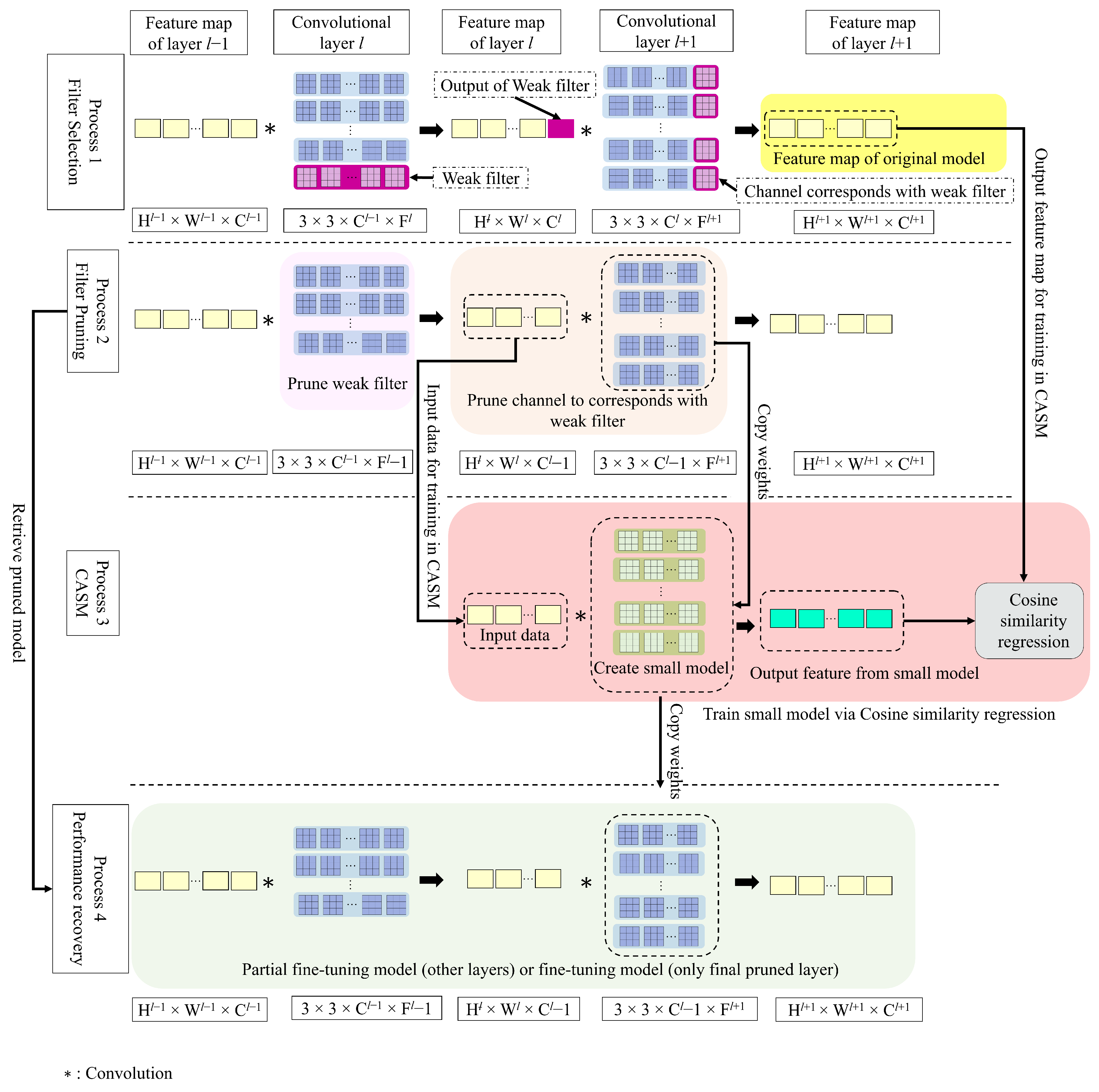
3.2. Convolutional Approximation of a Small Model (CASM)

CASM is a method for restoring kernel weights following the pruning process, as illustrated in Figure 2. Filters are assessed in process 1 (Filter Selection), and the results of weak filters are marked in purple highlighted blocks, where the dimension of the filter kernel is given as H, W: the height and width of the feature map, C: the number of filter channels, and F: the number of filters. In process 2 (Filter Pruning), highlighted weak filters in process 1 are removed from the CNN model while process 3 (CASM) performs convolution approximation of the kernels at layer $l+1$, which are affected by the reduction of output activations at layer l. As a result of the removal of the filter, only fragments of output activations remain, and partial convolutions are conducted at layer $l+1$. Due to the loss of activation output from layer l as the input to layer $l+1$, the remaining channel weights are no longer suitable to maintain layer performance. To restore the layer’s performance, the surviving channel weights must be relearned. We create a small model of a kernel based on the remaining structure of layer $l+1$, and we copy the remaining weights onto this small model. This small model is then trained using fundamental optimization in the spatial domain, with an objective function defined in Equation (4) [25].

$$J=\frac{1}{2}\left|\right|h\ast x-{y\left|\right|}^2$$

(4)

where J represents the objective function, h is the filter kernel of a small model, ∗ is convolution, x is the feature map of layer l from process 2 (Filter Pruning), and y is the output feature map of layer $l+1$ from process 1 (from original unpruned layer).

During the training process, kernel weight optimization is performed, and a cross-correlation (cosine similarity) metric (Equation (5)) is used as a performance assessment between the feature maps resulting from a small model and the original unpruned model. The optimization parameters are listed in

Table 1. A summarized table of optimization parameters for training CASM.

Parameter	Value
Optimizer	SGD
Learning rate	0.001
Momentum	0.9
Weight decay	0.0005
Epoch for training	500

.

The optimum weights of the small model are then reassigned to the pruned model at convolutional layer $l+1$ in process 4 (partial fine-tuning). In process 4, partial fine-tuning is executed from the initial layer up to convolutional layer $l+1$ (as depicted by the green highlighted block in Figure 2), encompassing all segments of the fully connected layer. Subsequent to the elimination of the final pruning layer, the model’s performance is reestablished through full fine-tuning. During this phase, all layers within the pruned model are unfrozen.

$$S=\frac{A·B}{\left|\right|A\left|\right|\left|\right|B\left|\right|}$$

(5)

where S represents cross-correlation (cosine similarity), A is a feature map from small model prediction and B is feature map $l+1$ from the original model.

4. Experiments and Discussion

This session evaluates the performance of the CASM framework using a CNN model that has been pre-trained via Keras library [27]. In Section 4.1, we explain the details of the pre-trained model and data to be implemented for the CASM framework evaluation experiment. In Section 4.2, we compare the results of CASM and its pruning model to those of other techniques utilizing basic or other frameworks.

4.1. A Detail of Experimental Implementation

The performance of the CASM framework was evaluated using two datasets and two pre-trained CNN models.

The utilized experimental datasets are the following:

• CIFAR-10 [28] is a small dataset, encompassing 32 × 32 pixel color images. This dataset contains 60,000 images with 10 different classes, with 50,000 allocated for training and 10,000 for testing.
• ImageNet (ILSVRC 2012) [29] is a large-scale dataset, consisting of 1.2 million images for the training set, with 1000 different classes, and 50,000 images for the validation set. The images are resized to 256 × 256 pixels, cropped to 224 × 224 pixels based on their centers, and horizontally flipped during the data augmentation process.

The utilized pre-trained CNN models are the following:

• VGG-16 [30] is a state-of-the-art CNN model designed for image classification. The basic structure consists of 13 convolutional layers and was designed to be used with large-scale image datasets. In each layer, the size of the kernel is 3 × 3. The performance of VGG-16 for image classification is outstanding. It was trained on datasets from ImageNet to CIFAR-10 [31] by reducing the number of object classes in the fully connected layer from 1000 to 10. In addition, a batch normalization layer [32] and a dropout layer [33] were added to each convolutional layer. All convolutional layers of VGG-16 on CIFAR-10 have parameters of 1.5 × 10${}^7$ and FLOPs (Floating Point Operation) of 6.3 × 10${}^8$. In this article, we equated 2× Multiply-Accumulate Computations (MACs) with FLOPs.
• ResNet-50 [12] is a state-of-the-art CNN model that is produced with a baseline of VGG-16 and 16 unique structures called residue blocks. This model can only have the first two convolutional layers of each block pruned, as the final convolutional layer cannot be pruned due to its unique structure. If it is pruned, the output feature map of the final convolutional layer of the block will not be compatible with the output feature map from the shortcut connection due to their difference in dimension. ResNet-50 has 2.3 × 10${}^7$ parameters and 7.7 × 10${}^9$ FLOPs.

For VGG-16, pruning begins at the second convolutional layer. For partial-fine tuning, the optimizer is set to SGD, one epoch, 0.001 learning rate, 0.9 momentum, and 0.0005 weight decay. For the final layer, a ${10}^{-3}$ to ${10}^{-5}$ learning rate and forty epochs are implemented. The batch size for this operation is set to 32. We prune model VGG-16 at a ratio of 50%, pruning with a comparison of 32 and 128 batch sizes. The accuracy results are 92.07% and 92.1%, respectively, and are not statistically distinguishable. In the CASM process, the CIFAR-10 dataset is utilized with 5000 images for training and 1000 images for testing. For the filter selection procedure, 10 images per class were used. Since VGG-16 on CIFAR-10 requires less processing time to prune the model, we can experiment in detail using a pruning ratio of 10–90%. The pruning ratio is the same for all convolutional layers.

For ResNet-50, pruning begins at the first convolutional layer of the first residual block. For partial-fine tuning, the optimizer is set to SGD, one epoch, 0.0001 learning rate, 0.9 momentum, and 0.0005 weight decay. For the CASM process, the ImageNet dataset is utilized with 1600 for training and 400 for testing. The remaining parameters are the same as those used for VGG-16. Pruning ratios of 30%, 50%, and 70% are conducted for ResNet-50 due to the large processing time of pruning on ImageNet.

To evaluate the performance of CASM and the basic fine-tuning framework, we conducted experiments using the VGG-16 model on the CIFAR-10 dataset, with a pruning ratio of 50%. We randomly selected three sets of 200, 500, and 1000 images from the dataset for training the model. The fundamental training parameters, including the SGD optimizer, learning rate of 0.001, momentum of 0.9, and weight decay of 0.0005, were kept consistent for both frameworks.

Since the development time for the CASM framework is significantly shorter compared to basic fine-tuning, we carried out experiments to assess layer recovery performance and training time for each framework.

4.2. Pruning Model Results

In this section, we demonstrate the results of CASM and the CASM framework’s pruning of the VGG-16 and ResNet-50 models.

4.2.1. Kernel Recovery Results of CASM

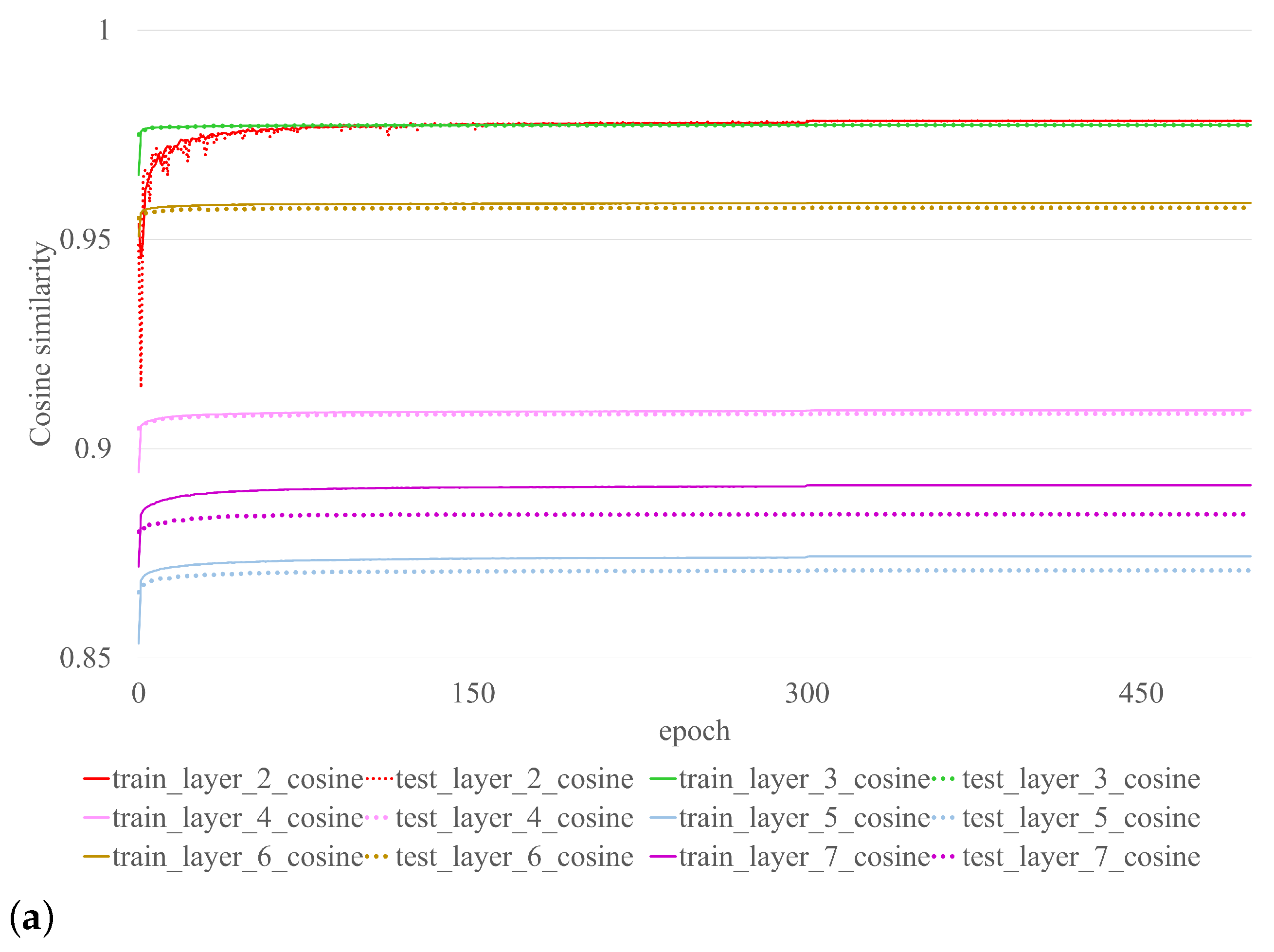
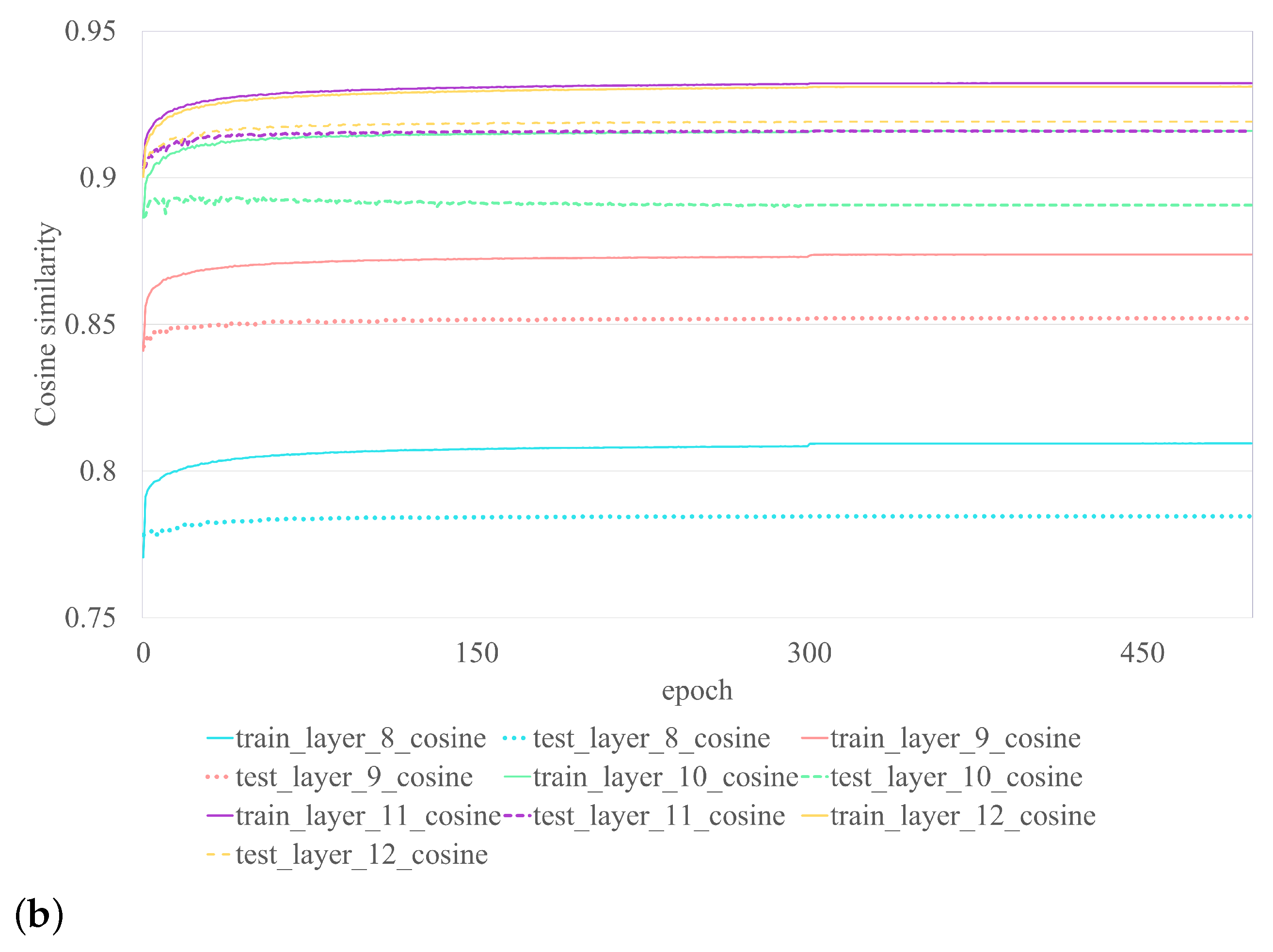
Cosine similarity is used to evaluate kernel recovery performance. The measurement reflects how close the results of the restored kernel are to those of the original kernel prior to pruning. Performance of the CASM on VGG-16 with CIFAR-10 is illustrated in Figure 3. Each color represents the outcome of each layer. The dotted line represents the training outcome, while the solid line represents the testing outcome of the CASM procedure. See also Figure 3a, which illustrates the outcome of layers 2–7 and Figure 3b, which illustrates the outcome of layers 8–12. Even though the CASM training results are nearly constant at epoch 300, as shown in Table 2, its performance has been satisfied since epoch 10. The final layer recovery is not performed due to absence of output activation at the subsequent layer of the original unpruned model used to train the small model. To achieve satisfactory performance, the CASM framework requires at least ten epochs, whereas the basic fine-tuning framework requires only one. However, as shown in Table 2, even with ten epochs of CASM training, the required time is significantly less than that of simple fine-tuning. With limited sample sizes (200, 500, 1000), CASM is able to regain performance that is superior to that of fine-tuning. Using the RTX 3090 (Nvidia Corporation, Santa Clara, CA, USA), we determined the average process time of all layers (see Table 2). CASM demonstrates superior processing speed compared to fine-tuning for different sample sizes. Specifically, for 200, 500, and 1000 samples, CASM processes 3.3 times, 2.4 times, and 1.7 times faster, respectively. The basic fine-tuning framework, on the other hand, requires a larger number of samples to achieve performance recovery. Even with 1000 samples, the performance of the basic framework did not match that of CASM, which utilized only 200 samples. CASM achieved superior performance, despite using less than five times the number of samples, and a performance gain greater than the basic fine-tuning framework, with a margin of 0.1498 (0.8050–0.6552). The superiority of CASM over basic fine-tuning becomes evident when considering the comparative aspects of sample size and processing time demanded by each approach.

Table 2. A performance comparison of layer-by-layer pruning using CASM and basic frameworks based on the pruned VGG-16 model with CIFAR-10 for 200, 500, and 1000 training samples.

Sample	State/Process	Layer 3	Layer 5	Layer 7	Layer 9	Layer 11	Layer 13
200	Before/CASM	0.8439	0.8431	0.7781	0.7755	0.8005	0.8050
	After/CASM	0.9220	0.8793	0.8076	0.8054	0.8041	0.8050 (1.25 s)
	Before/fine-tuning	0.4852	0.4637	0.3357	0.2522	0.4046	0.2251
	After/fine-tuning	0.5623	0.3410	0.2432	0.3346	0.3808	0.1961 (4.13 s)
500	Before/CASM	0.8418	0.8487	0.8016	0.8007	0.8238	0.8291
	After/CASM	0.9232	0.8859	0.8296	0.8270	0.8293	0.8291 (1.85 s)
	Before/fine-tuning	0.4496	0.5213	0.4081	0.3972	0.5648	0.4478
	After/fine-tuning	0.5922	0.5131	0.4926	0.4830	0.5865	0.5717 (4.35)
1000	Before/CASM	0.8498	0.8397	0.7774	0.8091	0.8350	0.8365
	After/CASM	0.9243	0.8902	0.8364	0.8389	0.8355	0.8365 (2.59 s)
	Before/fine-tuning	0.6569	0.6162	0.5068	0.5349	0.6206	0.6469
	After/fine-tuning	0.7498	0.6075	0.5602	0.6471	0.6651	0.6552 (4.43 s)

s represents seconds.

Table 2. A performance comparison of layer-by-layer pruning using CASM and basic frameworks based on the pruned VGG-16 model with CIFAR-10 for 200, 500, and 1000 training samples.

Sample	State/Process	Layer 3	Layer 5	Layer 7	Layer 9	Layer 11	Layer 13
200	Before/CASM	0.8439	0.8431	0.7781	0.7755	0.8005	0.8050
	After/CASM	0.9220	0.8793	0.8076	0.8054	0.8041	0.8050 (1.25 s)
	Before/fine-tuning	0.4852	0.4637	0.3357	0.2522	0.4046	0.2251
	After/fine-tuning	0.5623	0.3410	0.2432	0.3346	0.3808	0.1961 (4.13 s)
500	Before/CASM	0.8418	0.8487	0.8016	0.8007	0.8238	0.8291
	After/CASM	0.9232	0.8859	0.8296	0.8270	0.8293	0.8291 (1.85 s)
	Before/fine-tuning	0.4496	0.5213	0.4081	0.3972	0.5648	0.4478
	After/fine-tuning	0.5922	0.5131	0.4926	0.4830	0.5865	0.5717 (4.35)
1000	Before/CASM	0.8498	0.8397	0.7774	0.8091	0.8350	0.8365
	After/CASM	0.9243	0.8902	0.8364	0.8389	0.8355	0.8365 (2.59 s)
	Before/fine-tuning	0.6569	0.6162	0.5068	0.5349	0.6206	0.6469
	After/fine-tuning	0.7498	0.6075	0.5602	0.6471	0.6651	0.6552 (4.43 s)

s represents seconds.

4.2.2. Pruning Performance of VGG-16 on CIFAR-10

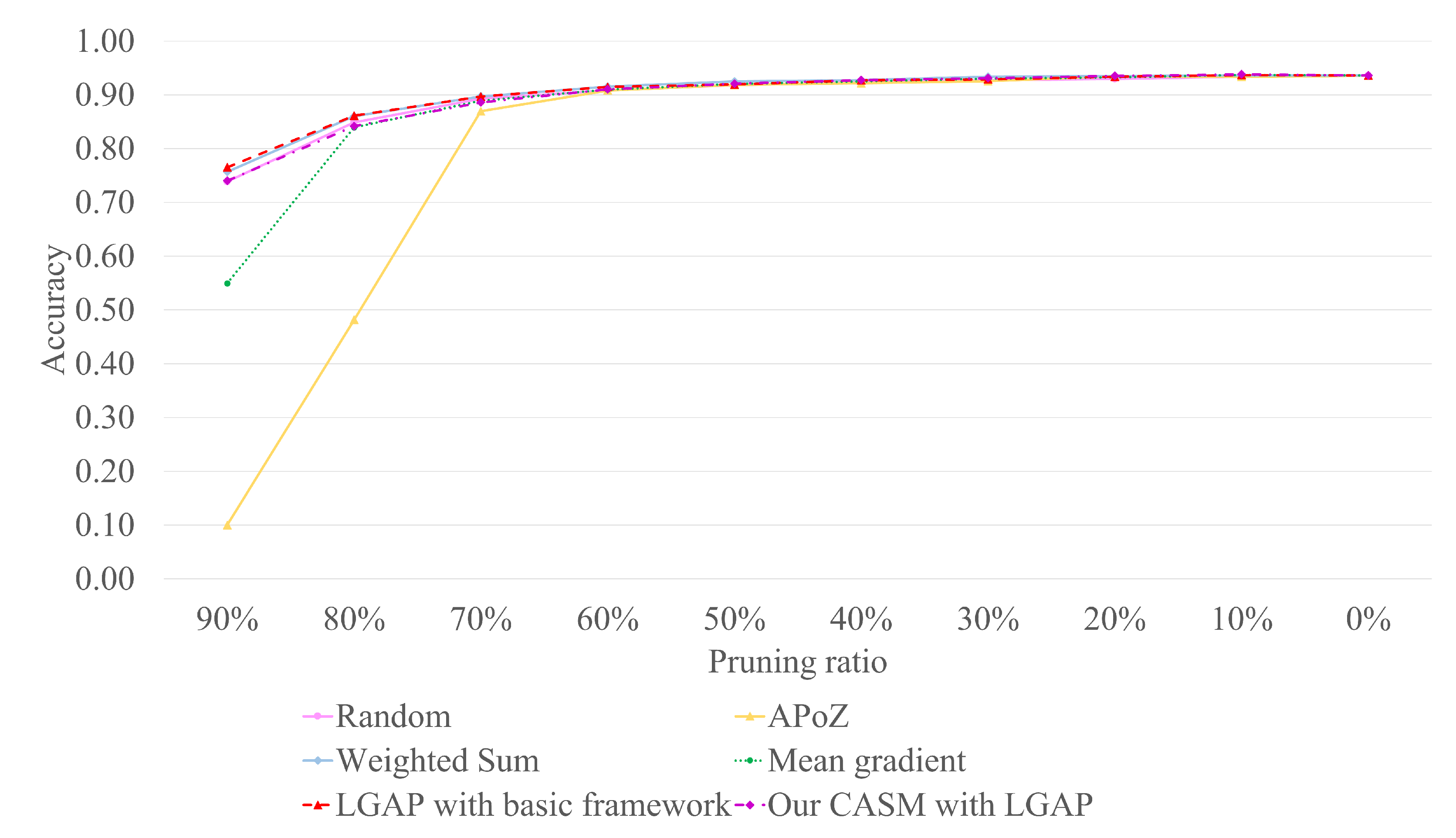
Table 3 illustrates the results of LGAP’s pruning with a combination of either the basic fine-tuning framework or the CASM framework. The results indicate that LGAP with CASM produces fewer errors than LGAP with the basic framework for pruning ratios less than or equal to 50%. With the range of 10% to 50% pruning ratio, the different errors between the basic and CASM frameworks are 0.13%, 0.17%, 0.24%, 0.03%, and 0.14%, respectively. At a 20% pruning ratio, the result of CASM pruning is roughly equivalent to the original model. This indicates that the CASM framework could restore excellent performance with a pruning ratio of 50% or less. If the pruning ratio is greater than 50%, the recovery performance of the CASM framework tends to degrade. Therefore, we would suggest using the CASM framework for a pruning ratio of 50% or less. Pruning VGG-16 could reduce FLOPs, number of parameters, and storage by 3.6×, 3.9×, and 3.9×, respectively, at a pruning ratio of 50%. Figure 4 illustrates a comparison of the performance of our LGAP with either the CASM or the basic framework and other pruning techniques: Random, Weighted sum, APoZ, and Mean gradient. It can be seen that at a pruning ratio less than or equal to 50%, the performances of all techniques are comparable.

Table 3. Pruning performance comparison of LGAP with basic framework and CASM framework based on VGG-16.

Technique, Framework	Pruning Ratio	Error (%)	FLOPs	FLOPs Reductions (×)	Parameters	Parameter Reductions (×)	Storage Size (MB)	Storage Reductions (×)
-	0%	6.41	6.3 × 10${}^8$	0	1.5 × 10${}^7$	0	57.4	0.0
LGAP, Basic	10%	6.32	5.1 × 10${}^8$	1.2	1.2 × 10${}^7$	1.2	46.2	1.2
LGAP, CASM		6.19
LGAP, Basic	20%	6.64	4.1 × 10${}^8$	1.5	9.6 × 10${}^6$	1.6	36.6	1.6
LGAP, CASM		6.47
LGAP, Basic	30%	7.12	3.2 × 10${}^8$	2.0	7.4 × 10${}^6$	2.0	28.2	2.0
LGAP, CASM		6.88
LGAP, Basic	40%	7.28	2.4 × 10${}^8$	2.6	5.4 × 10${}^6$	2.8	20.9	2.8
LGAP, CASM		7.25
LGAP, Basic	50%	8.07	1.7 × 10${}^8$	3.6	3.8 × 10${}^6$	3.9	14.6	3.9
LGAP, CASM		7.93
LGAP, Basic	60%	8.53	1.2 × 10${}^8$	5.4	2.4 × 10${}^6$	6.2	9.4	6.1
LGAP, CASM		8.97
LGAP, Basic	70%	10.34	7.2 × 10${}^7$	8.7	1.4 × 10${}^6$	10.8	5.5	10.5
LGAP, CASM		11.41
LGAP, Basic	80%	13.88	3.7 × 10${}^7$	16.9	6.4 × 10${}^5$	23.5	2.6	22.2
LGAP, CASM		15.82
LGAP, Basic	90%	23.48	1.4 × 10${}^7$	44.1	1.8 × 10${}^5$	84.4	0.8	69.5
LGAP, CASM		25.97

× is times. MB is Megabyte.

Table 3. Pruning performance comparison of LGAP with basic framework and CASM framework based on VGG-16.

Technique, Framework	Pruning Ratio	Error (%)	FLOPs	FLOPs Reductions (×)	Parameters	Parameter Reductions (×)	Storage Size (MB)	Storage Reductions (×)
-	0%	6.41	6.3 × 10${}^8$	0	1.5 × 10${}^7$	0	57.4	0.0
LGAP, Basic	10%	6.32	5.1 × 10${}^8$	1.2	1.2 × 10${}^7$	1.2	46.2	1.2
LGAP, CASM		6.19
LGAP, Basic	20%	6.64	4.1 × 10${}^8$	1.5	9.6 × 10${}^6$	1.6	36.6	1.6
LGAP, CASM		6.47
LGAP, Basic	30%	7.12	3.2 × 10${}^8$	2.0	7.4 × 10${}^6$	2.0	28.2	2.0
LGAP, CASM		6.88
LGAP, Basic	40%	7.28	2.4 × 10${}^8$	2.6	5.4 × 10${}^6$	2.8	20.9	2.8
LGAP, CASM		7.25
LGAP, Basic	50%	8.07	1.7 × 10${}^8$	3.6	3.8 × 10${}^6$	3.9	14.6	3.9
LGAP, CASM		7.93
LGAP, Basic	60%	8.53	1.2 × 10${}^8$	5.4	2.4 × 10${}^6$	6.2	9.4	6.1
LGAP, CASM		8.97
LGAP, Basic	70%	10.34	7.2 × 10${}^7$	8.7	1.4 × 10${}^6$	10.8	5.5	10.5
LGAP, CASM		11.41
LGAP, Basic	80%	13.88	3.7 × 10${}^7$	16.9	6.4 × 10${}^5$	23.5	2.6	22.2
LGAP, CASM		15.82
LGAP, Basic	90%	23.48	1.4 × 10${}^7$	44.1	1.8 × 10${}^5$	84.4	0.8	69.5
LGAP, CASM		25.97

× is times. MB is Megabyte.

4.2.3. Pruning Performance of ResNet-50 on ImageNet

Table 4. Pruning performance comparison of LGAP with basic framework and CASM framework based on ResNet-50.

Framework	Pruning Ratio	Top-1 Error (%)	Top-5 Error (%)	FLOPs	Parameters	Storage Size (MB)
-	0%	25.10	7.90	7.7 × 10${}^9$	2.6 × 10${}^7$	98.2
Basic	30%	27.55	8.94	4.8 × 10${}^9$	1.7 × 10${}^7$	65.2
CASM		26.80	8.67
Basic	50%	28.66	9.79	3.4 × 10${}^9$	1.2 × 10${}^7$	47.8
CASM		28.53	9.71
Basic	70%	31.44	11.26	2.2 × 10${}^9$	8.7 × 10${}^6$	33.6
CASM		31.47	11.45

Top-1 represents the highest probability (top-ranked) prediction that corresponds with the ground truth. Top-5 represents the five highest probability predictions that correspond with the ground truth. MB represents Megabytes.

illustrates the performance of pruning Resnet-50 using the LGAP technique with a combination of either the CASM or the basic fine-tuning framework. The experimental results show that LGAP with the CASM framework can provide superior recovery performance by 0.75% (30% pruning ratio) and 0.13% (50% pruning ratio) fewer errors for the top-1 and 0.13% (30% pruning ratio) and 0.08% (50% pruning ratio) fewer errors for the top-5. However, when the pruning ratio exceeds 70%, the basic framework is superior to the CASM framework. We believe that after a substantial amount of pruning, there is insufficient data for recovery since only a small number of filters remained. Thus, the basic fine-tuning framework with a massive number of retraining samples and several retraining cycles continues to be essential.

In Table 5, we compare the performance of LGAP with CASM to those of other techniques. At a 50% pruning ratio, the Top-1 accuracy of LGAP with CASM is superior to Random, SSL, ThiNet, APoZ, weighted sum, SSR-L2, Gradient mean, and LGAP with a basic framework by 1.22%, 1.15%, 0.69%,0.82%, 0.88%, 0.22%, 0.47%, and 0.13%, respectively. For top-5 accuracy, LGAP with CASM outperforms Random, SSL, ThiNet, APoZ, weighted sum, SSR-L2, Gradient mean, and LGAP with the basic framework by 0.94%, 0.87%, 0.47%, 0.60%, 0.61%, 0.30%, 0.13%, and 0.08%, respectively. ResNet-50 with 50% pruning can help reduce FLOPs, number of parameters, and storage by 2.3×, 2.1×, and 2.1×, respectively. The random technique for filter selection in model pruning is considered unstable, given its potential to yield either the best or the worst outcomes. It possesses the capacity to prune both robust and weak filters from the model. Although SSL can perform model pruning, it frequently alters the original model structure. The weighted sum approach relies on statistical weights to evaluate filters, constraining its ability to comprehend the spatial correlations and behavior of filters within a layer. Data-driven methodologies like ThiNet, APoZ, SSR-L2, Gradient Mean, and LGAP have demonstrated superior performance when compared to using only weight analysis. APoZ assesses filters based on the average percentage of zero activations within the activation layer. However, it fails to distinguish between two filters sharing the same zero activation area, potentially resulting in suboptimal pruning choices. Techniques such as ThiNet, SSR-L2, and Gradient Mean analyze filters using output feature maps and gradients, leading to a deeper grasp of filter significance in contrast to APoZ. Nevertheless, these methods still lack spatial relationship corresponding to target prediction.

In contrast, LGAP can analyze the spatial relationships among filters in each layer in a data-driven manner. Unlike methods that focus on a single weak filter, LGAP emphasizes distinct weak filters, allowing for the identification of crucial areas for target prediction. Consequently, LGAP demonstrates superior performance compared to alternative techniques [16].

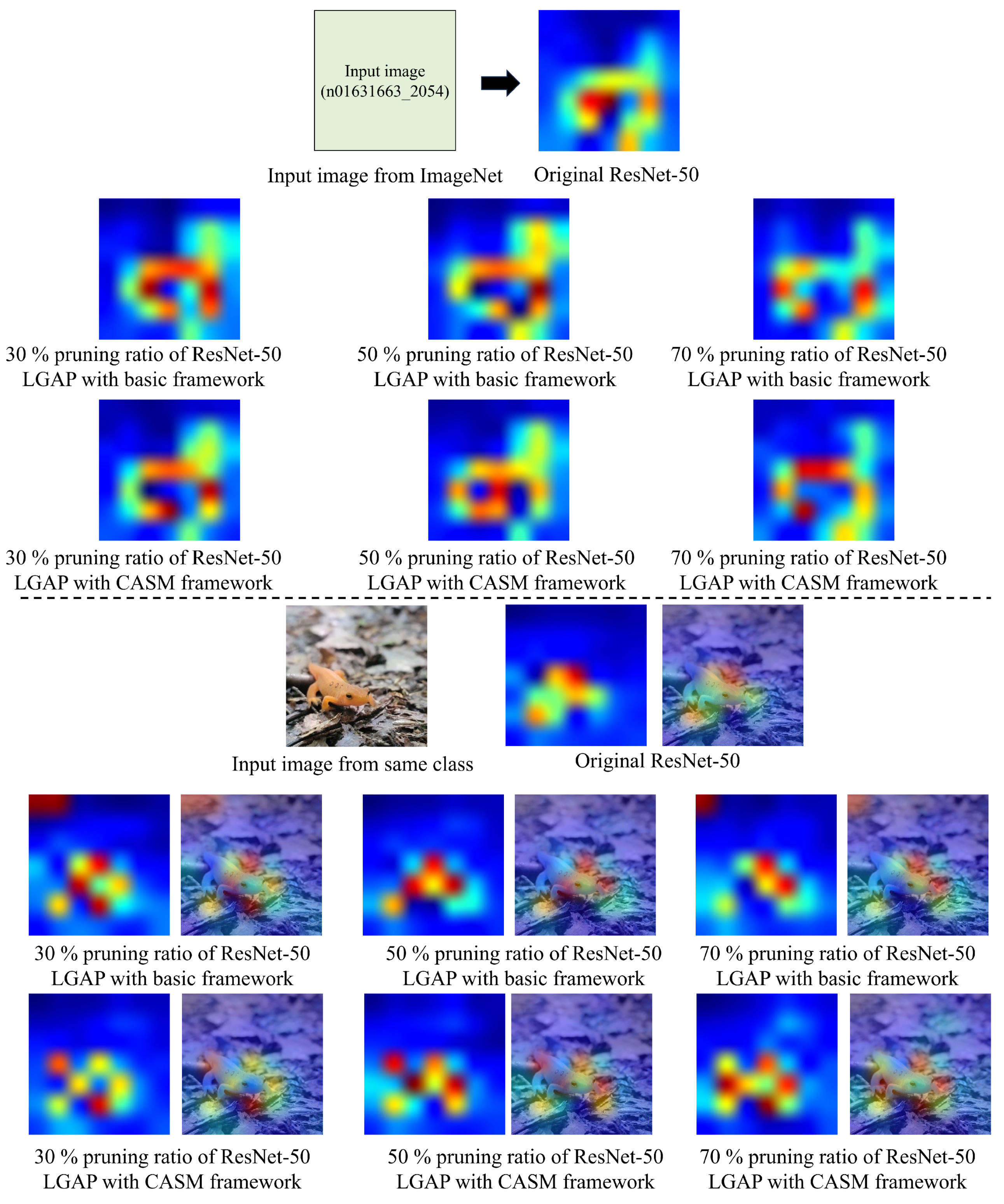
Figure 5 illustrates the visualization of the feature maps resulting from the pruned ResNet-50 using LGAP with either the CASM framework or the basic fine-tuning framework and the original model at different pruning ratios (30%, 50%, and 70%). When gradient localization was applied to LGAP and the basic fine-tuning framework with a 30% pruning ratio, our past research showed that the gradient localization of the model derived from both frameworks was comparable to that of the original model. However, during these experiments, we have observed that some sample images resulted in more gradient localization deviations with improved performance, such as the input image of class n01631663 in Figure 5 (upper). Additionally, we discovered that even when using data from the same class but sourced from outside ImageNet, the results still followed the same trend, as seen in Figure 5 (lower). These results indicate that such images can be effectively utilized for our purposes. The F1-score of the original model is 0.771 while the F1-scores of 30%, 50%, and 70% pruning ratios for LGAP with a CASM framework are 0.776, 0.796, and 0.817, respectively and for LGAP with a basic framework, they are 0.766, 0.804, and 0.787, respectively. When the compression ratio increased, the gradient localization varied more from the original model, as seen in Figure 5. Even at a pruning ratio of 70%, the F1-score of LGAP with CASM is proven to be superior to the original model and other pruned models. Even though pruning performance degrades at a high pruning ratio, some classes may outperform models with a lower pruning ratio or the original model. In addition, we analyzed the results from pruning the ResNet-50 model obtained from CASM and the basic framework in

Table 6. Cosine similarity of the output feature map at the final activation layer after pruning all layers was compared between the original model and CASM and basic framework on ResNet-50.

Pruning Ratio (%)	CASM Framework	BASIC Framework
30	0.6970	0.6752
50	0.6105	0.5996
70	0.5076	0.5087

. We fed two images per class (2000 images) from the validation set into the network of the original model, pruned the model by CASM and pruned the model by basic framework to obtain the output feature map from the final activation layer of each model. Cosine similarity is used to compare the similarity of the output feature map from the original model and pruned models (pruning by CASM and basic framework). We found that the cosine similarity between the original model and the pruned model by CASM at 30% and 50% pruning ratios was higher than the cosine similarity of the original model and the pruned model by the basic framework. This shows that pruning the model by the basic framework has a greater impact on changes from the original in the output feature map than CASM. When using the basic framework, all the layers are fine-tuned, which causes significant shifts in the model weights. Moreover, the time complexity of the basic framework is relatively high due to the fact that some of the layers are sensitive to being retrained and require additional fine-tuning (more than one epoch). In contrast, CASM attempts to restore performance by training the layer adjacent to the pruned layer and fine-tuning just certain parts of the model.

Table 5. Performance comparison of pruned ResNet-50 using LGAP with either CASM or basic framework with other pruning techniques at 50% pruning ratio.

Technique	Top-1 Accuracy Decrease (%)	Top-5 Accuracy Decrease (%)	FLOPs	Parameters	Pruned
Random	4.65%	2.75%	3.4 × 10${}^9$	1.2 × 10${}^7$	50%
SSL [19]	4.58%	2.68%	4.2 × 10${}^9$	1.3 × 10${}^7$	≈50%
ThiNet [23]	4.12%	2.28%	3.4 × 10${}^9$	1.2 × 10${}^7$	50%
APoZ [21]	4.25%	2.41%	3.4 × 10${}^9$	1.2 × 10${}^7$	50%
Weighted sum [20]	4.31%	2.42%	3.4 × 10${}^9$	1.2 × 10${}^7$	50%
SSR-L2 [24]	3.65%	2.11%	3.4 × 10${}^9$	1.2 × 10${}^7$	50%
Gradient Mean [22]	3.90%	1.94%	3.4 × 10${}^9$	1.2 × 10${}^7$	50%
LGAP with basic framework [16]	3.56%	1.89%	3.4 × 10${}^9$	1.2 × 10${}^7$	50%
LGAP with CASM framework	3.43%	1.81%	3.4 × 10${}^9$	1.2 × 10${}^7$	50%

Top-1 represents the highest probability (top-ranked) prediction that corresponds with the ground truth. Top-5 represents the five highest probability predictions that correspond with the ground truth.

Table 5. Performance comparison of pruned ResNet-50 using LGAP with either CASM or basic framework with other pruning techniques at 50% pruning ratio.

Technique	Top-1 Accuracy Decrease (%)	Top-5 Accuracy Decrease (%)	FLOPs	Parameters	Pruned
Random	4.65%	2.75%	3.4 × 10${}^9$	1.2 × 10${}^7$	50%
SSL [19]	4.58%	2.68%	4.2 × 10${}^9$	1.3 × 10${}^7$	≈50%
ThiNet [23]	4.12%	2.28%	3.4 × 10${}^9$	1.2 × 10${}^7$	50%
APoZ [21]	4.25%	2.41%	3.4 × 10${}^9$	1.2 × 10${}^7$	50%
Weighted sum [20]	4.31%	2.42%	3.4 × 10${}^9$	1.2 × 10${}^7$	50%
SSR-L2 [24]	3.65%	2.11%	3.4 × 10${}^9$	1.2 × 10${}^7$	50%
Gradient Mean [22]	3.90%	1.94%	3.4 × 10${}^9$	1.2 × 10${}^7$	50%
LGAP with basic framework [16]	3.56%	1.89%	3.4 × 10${}^9$	1.2 × 10${}^7$	50%
LGAP with CASM framework	3.43%	1.81%	3.4 × 10${}^9$	1.2 × 10${}^7$	50%

Top-1 represents the highest probability (top-ranked) prediction that corresponds with the ground truth. Top-5 represents the five highest probability predictions that correspond with the ground truth.

The introduction of the CASM has led to significant improvements in both performance and efficiency compared to the original model. By minimizing the deviation of the output feature map, CASM achieves greater similarity and improved accuracy. The CASM framework offers not only improved performance but also a significant reduction in time complexity, achieving a speed increase of 3.3 times compared to the basic framework. Moreover, CASM exhibits a capability to achieve higher model accuracy with a smaller dataset as compared to the basic framework (Table 2). With the integration of CASM into the pruning technique, our LGAP filter pruning becomes more effective, while ensuring that computational resources such as FLOPs and storage space remain consistent with the basic framework.

Figure 5. Visualization of feature map results from our pruned models with 30%, 50%, and 70% pruning ratio. The input image (n01631663_2054) is an image from the ImageNet [29] and the input image from the same class is from [34].

Figure 5. Visualization of feature map results from our pruned models with 30%, 50%, and 70% pruning ratio. The input image (n01631663_2054) is an image from the ImageNet [29] and the input image from the same class is from [34].

However, it is essential to note that CASM has a limitation when the pruned model exceeds a 50% threshold. In such cases, the recovery performance tends to deteriorate due to an insufficient number of channels in the remaining weights of the convolutional layer. This makes it difficult to accurately reconstruct the output feature map, as illustrated in Table 6. Despite this limitation, CASM’s overall contributions to performance enhancement, efficiency, and resource preservation make it a valuable addition to the existing framework.

5. Conclusions

In this research, we propose a new filter pruning framework for CNN models. Our new framework, known as the CASM framework, is a kernel recovery process, which creates a small model of remaining kernels. The kernel weights of the small model are fine-tuned to restore the feature map of the remaining kernel as closely as possible to that of the original unpruned kernel. With the same amount of training samples, CASM yields better results than the basic fine-tuning framework, while demanding less computational effort. The results clearly indicate that the CASM framework can restore the performance of a pruned model more effectively than the basic framework, especially at a pruning ratio of 50% or lower. This holds true for both VGG-16 with CIFAR-10 and ResNet-50 with ImageNet. Hence, CASM assists in recovering the remaining kernels with reduced complexity, fewer training samples, and less storage usage compared to the basic fine-tuning framework. The experimental results demonstrate CASM’s superiority over the basic fine-tuning framework, showing faster time acceleration (3.3×), requiring a smaller dataset volume for performance recovery post-pruning, and enhancing accuracy. For future research, we plan to explore a new framework for minimizing the time required to restore a pruned model’s performance by reducing both partial and full fine-tuning processes.