Abstract
We consider the multispecies model described by a coupled system of diffusion–reaction equations, where the coupling and nonlinearity are given in the reaction part. We construct a semi-discrete form using a finite volume approximation by space. The fully implicit scheme is used for approximation by time, which leads to solving the coupled nonlinear system of equations at each time step. This paper presents two uncoupling techniques based on the explicit–implicit scheme and the operator-splitting method. In the explicit–implicit scheme, we take the concentration of one species in coupling term from the previous time layer to obtain a linear uncoupled system of equations. The second approach is based on the operator-splitting technique, where we first solve uncoupled equations with the diffusion operator and then solve the equations with the local reaction operator. The stability estimates are derived for both proposed uncoupling schemes. We present a numerical investigation for the uncoupling techniques with varying time step sizes and different scales of the diffusion coefficient.
1. Introduction
Mathematical models used in various scientific disciplines, including chemistry, geology, ecology, and biology, incorporate reaction terms [1,2,3]. In mathematical ecology, reaction–diffusion models are employed to understand and describe the dynamics of species populations [4,5]. Spatial–temporal Lotka–Volterra models are utilized to investigate the populations of multiple interacting communities, considering the influence of spatial relationships on diverse aspects such as biodiversity and the structure of food webs [6]. The application of these models to marsh ecosystems at the mouth of the Nueces River is presented in [7]. Furthermore, one- and two-species population competition models are studied through unsteady diffusion–reaction equations [8,9]. In simulating subsurface flow and transport, reactive transport models capture the effects of biochemical reactions [10,11,12].
The reaction term is nonlinear and usually has a different time scale, requiring special numerical techniques for accurate and computationally effective solution development. To solve a nonlinear problem, a linearization technique is required. The Newton’s method is the traditional choice but is computationally expensive and sometimes requires small stepping for an accurate solution and method convergence. The Newton’s method, a powerful iterative technique for solving nonlinear equations, finds widespread use in scientific computation, despite its computational expense. It has proven valuable in diverse domains such as Computational Fluid Dynamics (CFD), Structural Mechanics, Electromagnetics, Geophysical Modeling, Optimization, Chemical Engineering, Climate Modeling, and Biomedical Simulations. Researchers often combine Newton’s method with optimization techniques, preconditioners, or adaptive step-size control to enhance its efficiency and overcome convergence challenges. Its effectiveness in tackling fully-implicit nonlinear problems remains a compelling choice for many scientific applications [13,14,15].
The most straightforward technique for solving nonlinear problems is linearization using a previous time-layer solution [16]. In the semi-implicit time approximation method, the reaction term is approximated using the solution from the previous time layer [17,18,19,20]. This approach is beneficial when applied to multispecies interaction models, as it leads to uncoupled equations for each species. This uncoupling improves computational efficiency and enables faster simulations than fully coupled and implicit schemes. Operator-splitting methods have been extensively employed in computational mathematics [21,22,23]. These methods divide coupled multiphysics processes into components corresponding to different physical processes, allowing each component to be treated with specific techniques [24]. Such schemes have been developed for various problems, including convection–diffusion–reaction problems, Navier–Stokes equations, poroelasticity, and thermoelasticity problems [18,24,25,26,27,28,29]. The splitting methods allow different numerical methods and libraries to solve the subproblems, reducing computational effort for large problems and enabling parallel computations.
Additive operator-difference schemes are valuable for solving unsteady equations in the context of time approximation. These schemes can be effectively combined with explicit–implicit time approximation methods. Explicit–implicit time approximation is commonly employed for convection–diffusion–reaction equations [10,17,18,25,30]. Reactive transport processes often involve a combination of slow transport processes and stiff reaction terms. In such cases, explicit time approximation methods can approximate the slow transport processes, while the fast reaction terms are treated implicitly [10]. The explicit–implicit scheme is applied to decouple equations in the context of multicontinuum flow problems in fractured porous media in the study mentioned in [17].
In this work, we consider uncoupling techniques for the multispecies model. This mathematical model is described by a coupled system of reaction–diffusion equations, where the system’s nonlinearity is related to the reaction term. We start with a standard fully implicit approach with the Backward Euler time approximation and Newton solver. Then, we consider two schemes useful for uncoupling systems and linearizing the nonlinear reaction term. We first consider linearization based on evaluating a part of the reaction term using the solution from the previous time layer (explicit–implicit scheme). In this approach, we take the concentration of another species in coupling term from the previous time layer to obtain a linear uncoupled system of equations, i.e., we solve the equation for each species separately. The second approach is based on the operator-splitting technique, where we first apply a diffusion operator and then apply a local reaction operator that can be calculated using explicit or implicit time approximation in each grid cell separately (local problem). Operator splitting techniques lead to the uncoupled system, where each species’ diffusion equation is solved separately. We present a numerical investigation of the uncoupling techniques with varying time step sizes and different scales of diffusion coefficients.
This paper is organized as follows. In Section 2, we describe the problem formulation with a finite volume approximation by space and a fully implicit approximation by time. The uncoupling techniques are presented in Section 3. A numerical investigation of the methods’ accuracy with computational effectiveness is presented in Section 4. The paper ends with a conclusion.
2. Problem Formulation
We consider the multispecies competition model that is described by the following system of equations:
where is the population of the kth species, is the diffusion coefficient, is the kth population reproductive growth rate, and is the interaction coefficient due to competition ( compete with ).
The system of equations is considered with initial conditions
and free boundary conditions
where n is the outer normal vector to the boundary .
2.1. Approximation by Space
For the numerical solution of the problem Equation (1) with initial and boundary conditions Equations (2) and (3), we use a finite volume method for approximation by space [31].
Let be the triangulation of the domain with mesh size h
where is the grid cell, , and N is the number of the grid cells. Let be the interface (facet) between two cells and , .
Let be the cell average value of the function on cell
where is cell volume.
For diffusion, we use a two-point flux approximation,
where is the distance between cell center points and , is the length of the interface between cells and , and is the harmonic average, .
Therefore, we have the following semi-discrete form:
Next, we consider implicit time approximation to construct a discrete system of equations.
2.2. Fully Implicit Scheme for Approximation by Time
Let and , where , and is the fixed time step size. For approximation by time, we apply an implicit scheme and obtain the following discrete system:
To solve a nonlinear system of equations, we use the Newton method.
Let s be the nonlinear iteration number and
where .
In the considered problem, we have a linear diffusion operator and the following nonlinear reaction operator:
In Newton’s method, we apply the following linearization
and obtain the following system of linear equations on each nonlinear iteration
with
for . We iterate nonlinear iterations until becomes smaller than the given tolerance or until we reach a maximum nonlinear iteration. We use a solution from the previous time layer as an initial condition in nonlinear iterations. The scheme Equation (6) is a fully implicit approximation, FI (coupled).
3. Uncoupling Techniques
In the fully implicit approximation by time, we update the matrix and right-hand side of the linear system of equations in each time and nonlinear iteration, which is computationally expensive. Furthermore, the convergence of the nonlinear iterations depends on the time step size, and for larger time steps, it takes more iterations to converge. Note that the Newton method is the most accurate method for the solution of the nonlinear system of equations, and we will use it to calculate the reference solution by setting a small time step. In this section, we construct uncoupling techniques that are more computationally effective. We start with the most straightforward scheme constructed by linearization from the previous time layer.
3.1. Semi-Implicit Schemes
To construct semi-implicit schemes by time (linearized scheme), we take some of the parameters in the reaction operator from the previous time step. By varying parameters that are linearized, we can obtain the following schemes:
- SI-1 (uncoupled):Here, we set the whole reaction term using the solution from the previous time layer. In the resulting scheme, the matrix of the system of linear equations that we solve at each time iteration is fixed and decoupled for each component (species). So, we can solve equations for each species separately by updating only the right-hand side vector.
- SI-2 (uncoupled):In this scheme, we still obtain decoupled problems for each species but approximate part of the reaction term using a current solution. Therefore, each iteration should update the matrix and right-hand side vector of the linear system of equations.
- SI-3 (coupled):Here, we obtain a coupled problem for the multispecies competition model, but this problem is linear in each iteration. We will use it in the numerical investigation and compare it with other schemes.
Note that the main characteristic we want to reach is the separate solution of the equation for each species (uncoupled scheme). By uncoupling the problem, we are constructing a fast computational algorithm.
To write stability estimates for the proposed schemes, we write all schemes in a unified way and introduce the following matrices:
For matrix , we define an uncoupled way of linearization (SI-1 and SI-2):
and coupled way of linearization (SI-3):
Then, we can rewrite the linearized system in the following matrix form [9,17]:
where , , , and are the weights.
Particularly, in this work, we set (implicit diffusive transport)
with and initial condition .
- SI-1 (uncoupled): where .
- SI-2 (uncoupled): with .
- SI-3 (coupled): with .
For the presented matrices, we have the following properties:
where is the indetity matrix, , , , and and (undimensional case).
To derive a stability estimate of the semi-implicit scheme Equation (14), we write a weighted scheme in the following form (a canonical form of two-level schemes) [18,32,33,34]
where
For the first scheme with (SI-1), we have
and
Next, after scalar multiplication by of Equation (17), we obtain
Taking into account that
we obtain
with .
Therefore, we have
Then, we can write the following stability estimate for the scheme SI-1 for .
Theorem 1.
The semi-implicit scheme of Equation (16) with (SI-1) is unconditionally ρ-stable and satisfies the following estimate:
with .
Finally, we consider schemes with (SI-2 and SI-3). Here, the operator in the problem in Equation (16) is not sign-definite, and for the solvability, we should ensure that . Using operator properties in Equation (15), we obtain
This leads to the following time step size restriction.
Note that a similar time step restriction was derived in our previous works [20,35] for convection–diffusion problems and can be found in [36,37] for reaction-diffusion problems.
Therefore, for the schemes SI-2 and SI-3, we seek a -stability estimate (see [18,20,32,33,34,35] for details). Let with . Substituting it into Equation (16), we obtain
with
Here, we can write
The stability of the scheme Equation (19) can be proven if the operator can be associated with . With
we obtain
Under the following conditions for
we have
Then, we have . Moreover, we have then . Finally, the following stability estimate is valid.
Theorem 2.
The semi-implicit scheme Equation (16) with (SI-2 and SI-3) is ρ-stable and satisfies the following estimate:
where and the time step satisfies constrain ().
3.2. Operator-Splitting Scheme
Next, we consider a fractional time stepping method based on the operator splitting technique. In this method, we first apply the diffusion operator, and after that the reaction operator, where the previous diffusive solution is used as an initial condition. The main advantage of the operator-splitting scheme is that we obtain an uncoupled system of equations for the multispecies interaction model. Furthermore, the second equation (reaction operator) is local, i.e., it does not depend on neighbor values of the solution and can be solved for each grid cell independently.
We have the following algorithm:
- 1.
- Solve parabolic PDEs for each species k independently to find ,with initial condition for .
- 2.
- Solve coupled nonlinear ODEs to find ,with initial condition for .
In this algorithm, we separate the system into diffusion and reaction parts, where the diffusion part in Equation (22) is uncoupled and solved using implicit approximation by time (Backward Euler, BE)
for each independently.
The coupled nonlinear local reaction part of Equation (23) can be solved using an implicit time-approximation scheme (BE):
for each cell independently. We note that the splitting scheme in Equations (24) and (25) has a first-order accuracy by [27,28,29].
To derive the stability estimate of the operator splitting scheme, we write the equation in the following form:
By the scalar multiplication of the equation by and , we obtain
Then, using the operator’s properties, we have
By the Cauchy–Schwarz inequality, we obtain
Finally, for , we have the following stability estimate
In the presented operator-splitting scheme, we can handle the time step restriction by performing a smaller time step size for the reaction subproblem and by keeping a more significant time step size for the diffusion subproblem. Such schemes are related to multirate time approximation schemes, where a different time step size can be used for each subproblem. Note that the explicit multistep methods can be used, whereas for the case of the one-step method, we can obtain the Forward Euler formula (FE). We note that, for FE approximation with fixed time step size , we obtain a similar time approximation as SI-1.
Furthermore, a general class of adaptive implicit multistep methods can be used for a set of local ODEs in Equation (23) in each cell . Particularly, we will use the adaptive backward differentiation formula (BDF) to solve ODEs in time interval with varying order p and time-step size [38,39,40]. Let for with and . Then, to find in each cell at time , we solve
with initial condition
with
Finally, we set . This method is implicit and requires the solution of nonlinear equations at each step. Note that the considered above Backward Euler scheme is equivalent to the BDF with (BDF1).
4. Numerical Results
For numerical investigation, we consider the multispecies interaction model in the heterogeneous domain . Let , where is the background subdomain and is the subdomain of the inclusions (see Figure 1). For the heterogeneous properties, we set:
where , , , , and are constants that characterize properties of the subdomains. We note that the solution to such problems requires the construction of grids that resolve heterogeneity on the grid level, which leads to a large system of equations that is computationally expensive to solve. The application of the Newton method requires even more computational time.
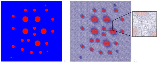
Figure 1.
Heterogeneous domain with fine grid that resolves heterogeneity on the grid level. Blue color: background subdomain, . Red color: subdomain of the circle inclusions, .
We consider the two-species competition model
with small, medium and large diffusions:
- Small diffusion (s)
- Medium diffusion (m)
- Large diffusion (l)
Note that the diffusion coefficients for the first and second species are opposite, i.e., we consider the case when the first species is less diffusive in the primary subdomain (background) with . We set the opposite case for the second species when background media are more diffusive .
We consider two test problems:
- Test 1and and 100 time iterations.
- Test 1s (small diffusion)
- Test 1m (medium diffusion)
- Test 1l (large diffusion)
- Test 2and and 100 time iterations.
- Test 2s (small diffusion)
- Test 2m (medium diffusion)
- Test 2l (large diffusion)
As the initial condition, we set . In both test problems, we simulate 100 time steps.
For constructing the computational geometry with inclusions and grid generation, we use Gmsh [41]. Numerical implementation is performed using PETSc [42,43] and FEniCS libraries [43,44]. To visualize the results, we use Paraview [45].
We solve the problem on the fine grid and use the solution as a reference solution to calculate the errors of the multiscale solver. The fine grid contains 69,948 cells and for each component. In Figure 2, we present the dynamic of the average values of the solution for Test 1 and 2 for cases with no diffusion (Test 1 (ODE) and 2 (ODE)), small (Test 1s and 2s), medium (Test 1m and 2m) and large diffusion (Test 1l and 2l). To calculate the average solution, we use the following formulas:
where and are the volume of the domains and , respectively. In Figure 2, we also present values of the solutions at the final time. Numerical solutions for small, medium, and large diffusion at the final time are presented in Figure 3 for Test 1 and 2. We observe a considerable influence of the diffusion on the solution in the inclusions subdomain. However, the effect of diffusion on the solution in the background domain is minor. We see that both species survive in background media in Test 1, but the population of the first species is smaller than that of the second. In Test 2, we observe that the population of the second species is very small, and the first species almost survives in background media. The influence of the diffusion in inclusions is very large and can change dominated species. For example, the first species dominate the second in Test 1 with no diffusion, but for a problem with diffusion, we see that the second species starts to dominate over the first. We observe similar behavior in the inclusions for Test 2.

Figure 2.
Dynamic of the average solution with no diffusion (ODE) and for small, medium and large diffusion using Newton’s method (FI, fully implicit, coupled). (left) and (right) (red color) and (blue color).
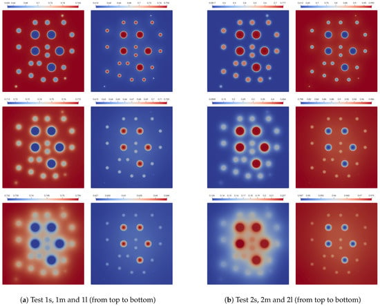
Figure 3.
Final time solution for small, medium and large diffusion using Newton’s method (FI, fully implicit, coupled). (left) and (right).
For the fully implicit scheme, we consider the effect of the time stepping size on the method accuracy. In Figure 4, we present the dynamic of the average values of the solution for Test 1 and 2 with and 10. We use a fully implicit scheme with the smallest as a reference solution. We observe that the more significant difference occurs at the first half-time of simulations.
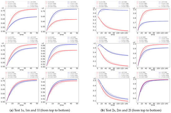
Figure 4.
Dynamic of the solution for small, medium and large diffusion using Newton’s method (FI, fully implicit, coupled). (left) and (right) (red color) and (blue color).
Next, we calculate the errors between the reference solution and the solution with a more significant time step size ( and 10). To compare solutions, we calculate relative errors for the first and second species populations using the following formulas:
where is the reference solution (coupled) and is the solution using uncoupling methods.
The error dynamic is presented in Figure 5 for Test 1 and 2. We observe significant errors at the beginning. We obtain more notable errors for the first species In Test 1. In Test 2, we obtain more significant errors for the second species. However, the error for the first species in Test 2 does not reduce by time.
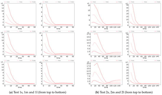
Figure 5.
Dynamic of the errors for small, medium and large diffusion using FI scheme. (left) and (right).
In Table 1, we present the time of calculations for the fully implicit scheme with different values of time step size . We also present the total number of linear system solutions directly affecting the solution time. We observe that the time of simulations is more significant for Test 2 due to the higher nonlinearity that leads to the larger number of linear system solutions (number of nonlinear solver iterations). Moreover, we see that the solution time is more significant for the more extensive diffusion. The effect of the time step size is represented, where a smaller time of calculations is needed for a more significant time step size.

Table 1.
Time of solution (sec) and total number of nonlinear iterations for Test 1 and 2 with small, medium and large diffusion using Newton’s method (FI, fully implicit, coupled). Number of time steps: 100 for , 50 for , 20 for and 10 for .
Next, we consider the solution to the problem using presented uncoupling techniques. We start with the semi-implicit schemes. In Figure 6, we depict the error dynamics for the three semi-implicit schemes. The results are presented for fixed time step size . The errors are calculated between the considered semi-implicit scheme and the fully implicit scheme with the same time step size . For Test 1, we observe minor errors for all three diffusions. In Test 2, we obtain more significant errors for all three semi-implicit schemes. The error behavior is similar for SI-1 and SI-2 in Tests 1 and 2. However, we observe a significant error at the final time for SI-3. In Test 2, the errors for SI-3 are more considerable for more extensive diffusion. SI-1 and SI-2 are preferable variances for the semi-implicit scheme because that leads to the uncoupled system. Note that the presented semi-implicit schemes are related to the simplest linearization, where the nonlinear part is taken from the previous time layer. In SI-1, we approximate the whole reaction term using the solution from the previous time layer. In this scheme, the matrix of the system of linear equations that we solve at each time iteration is fixed and decoupled for each component (species). In SI-2, we also have decoupled problems for each species but approximate part of the reaction term using a current solution. Therefore, each iteration should update the matrix and right-hand side vector of the linear system of equations. In SI-3, we have a coupled problem for the multispecies competition model, but each iteration is linear. The presented numerical results show that the SI-1 and SI-2 schemes give more minor errors than SI-3. Furthermore, because SI-1 and SI-2 schemes give almost the same errors, we can state that the SI-1 is preferable due to its most straightforward realization with a fully explicit approximation of the reaction part.
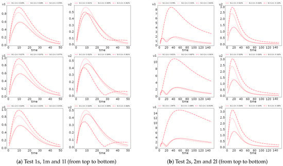
Figure 6.
Dynamic of the errors for small, medium and large diffusion using SI-1, SI-2 and SI-3 scheme with . (left) and (right).
The semi-implicit and operator splitting method results are presented in Figure 7. Note that we use the LSODE solver to solve the ODE system in the OS scheme. We depict the dynamics of the average solution for each species in each subdomain. The final average value of the solution is represented. The results for fully implicit, semi-implicit, and operator splitting methods are represented for . We observe a slight difference between solutions in Test 1 for small, medium, and large diffusion. However, the difference in the first half of time is slightly larger for more significant diffusion. In Test 2, we see good results for small diffusion. We observe a sufficiently big difference for larger diffusion, where larger errors occur for the operator-splitting method (OS). The difference between the fully implicit and operator-splitting method is more significant for the first species.
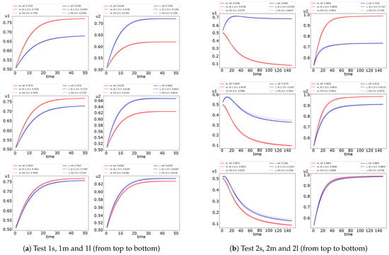
Figure 7.
Dynamic of the solution for small, medium and large diffusion using SI-1 and OS schemes. (left) and (right). (red color) and (blue color).
In Figure 8, we represent the error dynamic for the semi-implicit and operator splitting method. We see that the operator splitting method errors for the first species in Test 2 has an increasing behavior. Moreover, we obtain significant errors for a larger diffusion. For example, we obtain of error in Test 2l, of error in Test 2m and of error in Test 2s. The errors for both uncoupling methods are similar for Test 1, with less than one percent of errors. The results also illustrate that the operator splitting method is better than the semi-implicit approximation in Test 1. Nevertheless, in Test 2, we observe the opposite case with more minor errors for the semi-implicit scheme. The presented results of the errors also illustrate the dynamics of uncoupling errors, where the semi-implicit approach gives a more significant error in the first half of the simulation’s time and rapidly decreases after that. The operator splitting error dynamics is entirely different, where the accurate approximation is performed at the begging of the simulation time.
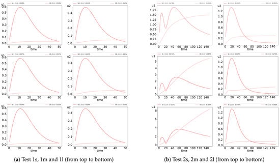
Figure 8.
Dynamic of the errors for small, medium and large diffusion using SI-1 and OS schemes with . (left) and (right).
In Figure 9 and Figure 10, we investigate the influence of the time step size on the SI-1 and OS method accuracy. Similarly to the fully implicit scheme, we observe more significant errors for Test 2. In Test 1, the errors are significant in the first half of the simulation’s time and converge to sufficiently small errors at the final time. However, in Test 2, we have a significant influence of the time step size on the method accuracy, especially for the first species.
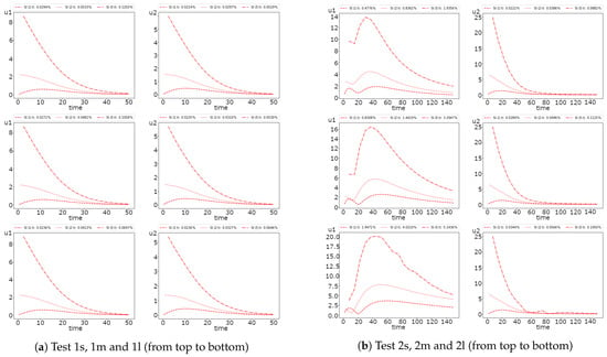
Figure 9.
Dynamic of the errors for small, medium and large diffusion using SI-1 scheme with and 10. (left) and (right).
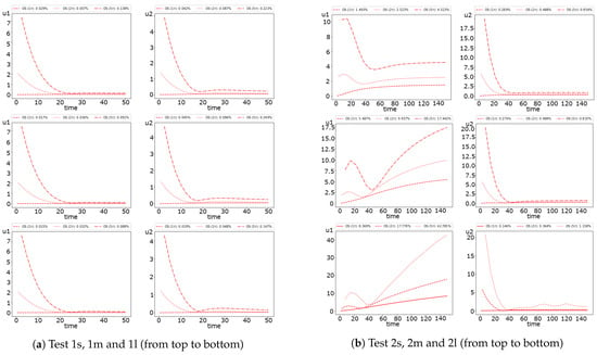
Figure 10.
Dynamic of the errors for small, medium and large diffusion using OS scheme with and 10. (left) and (right).
Finally, we present the solution time for uncoupled schemes and compare them with the fully implicit scheme. Note that the main characteristic we want to reach is the separate equation solution for each species (uncoupled scheme). By uncoupling the problem, we are constructing a fast computational algorithm. In Figure 11, we present a bar plot for calculation time for three semi-implicit schemes (SI-1, SI-2, and SI-3). We observe that the coupled scheme SI-3 leads to a slower computational algorithm due to the solution of the large coupled system at each time step. The decoupled approaches SI-1, and SI-2 are faster, where the fastest algorithm is related to the fully explicit approximation of the reaction term. We also observed from the previous numerical results that the SI-1 method has good accuracy for such problems. The time of calculations for the explicit–implicit scheme (SI-1), operator-splitting scheme(OS), and fully implicit scheme (FI) are presented in Figure 12. We note that the quickest algorithm is provided by the SI-1 method. For example, the solution time using the SI-1 scheme is approximately 49 and 64 s for small diffusion in Test 1 s and 2 s, respectively. For more significant diffusion values, we have more significant calculations time with 229 and 405 s for Test 1m and 2m (medium diffusion) and 57 and 76 s for Test 1l and 2l (large diffusion). Compared with the fully implicit scheme, we obtain a 37–38 times faster solution for SI-1 and a 3–4.3 faster solution for OS for small diffusion test cases. We have a 19–23 times faster solution for SI-1 and a 3.4 times faster solution for OS for the medium diffusion. For the large diffusion case, we have a 6.6–9.6 times faster solution for SI-1 and a 4.2 faster solution for OS. Therefore, the SI-1 scheme is preferable due to it having the most straightforward implementation and the faster solution. However, the accuracy highly depends on a test set of parameters, and the correct choice should be performed for each case.
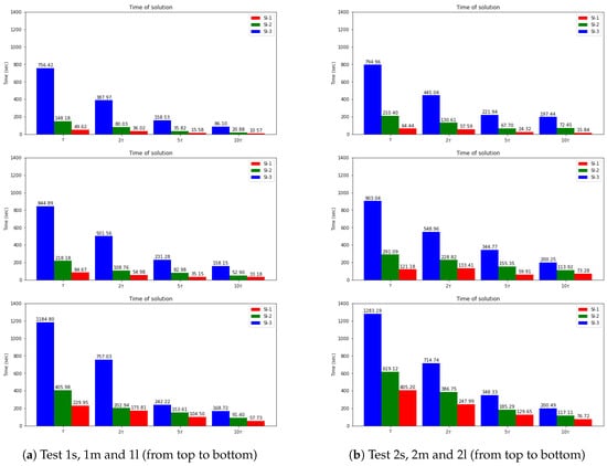
Figure 11.
Time of calculations. Dynamic of the errors for small, medium and large diffusion using SI-1, SI-2 and SI-3 schemes.
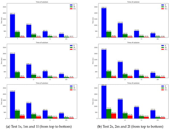
Figure 12.
Time of calculations. Dynamic of the errors for small, medium and large diffusion using FI, SI-1 and OS schemes.
5. Conclusions
The multispecies model was considered in the heterogeneous domain. The coupled system of reaction–diffusion equations was used to describe the mathematical model, where the coupling and nonlinearity are given in the reaction part. We constructed a semi-discrete form using a finite volume approximation by space. The fully implicit scheme was applied for approximation by time, which led to solving the nonlinear system of equations at each time step. We presented and investigated two uncoupling approaches for such problems based on the explicit–implicit scheme and the operator-splitting method. Three approaches were considered in the semi-implicit scheme: (SI-1) implicit diffusion and fully explicit reaction; (SI-2) implicit diffusion and partially explicit reaction (uncoupled); and (SI-3) implicit diffusion and partially explicit reaction (coupled). The operator-splitting scheme was based on decoupling the diffusive and reactive parts of the equation using the first-order sequential non-iterative technique. The numerical investigation was performed for two sets of parameters in a two-dimensional domain with heterogeneous inclusions. Three test cases with small, medium, and large diffusions were considered to illustrate the influence of the uncoupling method accuracy and computational time.
Author Contributions
Conceptualization, M.V. and A.S.; methodology and software, M.V.; validation and investigation, M.V., S.S. and S.H.; writing—original draft, M.V., S.S. and A.S.; writing—review and editing, M.V., S.S. and A.S. All authors have read and agreed to the published version of the manuscript.
Funding
The research of S.S. was funded by the Ministry of Education and Science of the Russian Federation under grant No. FSRG-2023-0025.
Data Availability Statement
Not applicable.
Conflicts of Interest
The authors declare no conflict of interest.
References
- Marchuk, G.I. Mathematical Models in Environmental Problems; Elsevier: Amsterdam, The Netherlands, 1986. [Google Scholar]
- Allaire, G.; Brizzi, R.; Mikelić, A.; Piatnitski, A. Two-scale expansion with drift approach to the Taylor dispersion for reactive transport through porous media. Chem. Eng. Sci. 2010, 65, 2292–2300. [Google Scholar] [CrossRef]
- Bhatnagar, G.; Chapman, W.G.; Dickens, G.R.; Dugan, B.; Hirasaki, G.J. Generalization of gas hydrate distribution and saturation in marine sediments by scaling of thermodynamic and transport processes. Am. J. Sci. 2007, 307, 861–900. [Google Scholar] [CrossRef]
- Okubo, A.; Levin, S.A. Diffusion and Ecological Problems: Modern Perspectives; Springer: Berlin/Heidelberg, Germany, 2001; Volume 14. [Google Scholar]
- Chairez, Z.P. Spatial-Temporal Models of Multi-Species Interaction to Study Impacts of Catastrophic Events. Ph.D. Thesis, Texas A&M University, Corpus Christi, TX, USA, 2020. [Google Scholar]
- Murray, J.D. Mathematical Biology: I. An Introduction; Springer: Berlin/Heidelberg, Germany, 2002. [Google Scholar]
- Montagna, P.A.; Sadovski, A.L.; King, S.A.; Nelson, K.K.; Palmer, T.A.; Dunton, K.H. Modeling the Effect of Water Level on the Nueces Delta Marsh Community. Wetl. Ecol. Manag. 2017, 25, 731–742. [Google Scholar] [CrossRef]
- Vasilyeva, M.; Wang, Y.; Stepanov, S.; Sadovski, A. Numerical investigation and factor analysis of the spatial-temporal multi-species competition problem. arXiv 2022, arXiv:2209.02867. [Google Scholar] [CrossRef]
- Vasilyeva, M.; Sadovski, A.; Palaniappan, D. Multiscale solver for multi-component reaction–diffusion systems in heterogeneous media. J. Comput. Appl. Math. 2023, 427, 115150. [Google Scholar] [CrossRef]
- Steefel, C.I.; MacQuarrie, K.T. Chapter 2. Approaches to modeling of reactive transport in porous media. In Reactive Transport in Porous Media; Lichtner, P., Steefel, C., Oelkers, E., Eds.; De Gruyter: Berlin, Germany; Boston, MA, USA, 2018; pp. 83–130. [Google Scholar] [CrossRef]
- Battiato, I.; Tartakovsky, D.M.; Tartakovsky, A.M.; Scheibe, T.D. Hybrid models of reactive transport in porous and fractured media. Adv. Water Resour. 2011, 34, 1140–1150. [Google Scholar] [CrossRef]
- Korneev, S.; Battiato, I. Sequential homogenization of reactive transport in polydisperse porous media. Multiscale Model. Simul. 2016, 14, 1301–1318. [Google Scholar] [CrossRef]
- Knoll, D.A.; Keyes, D.E. Jacobian-free Newton–Krylov methods: A survey of approaches and applications. J. Comput. Phys. 2004, 193, 357–397. [Google Scholar] [CrossRef]
- Knoll, D.; McHugh, P. Newton-Krylov methods applied to a system of convection-diffusion-reaction equations. Comput. Phys. Commun. 1995, 88, 141–160. [Google Scholar] [CrossRef]
- Macías-Díaz, J.E.; Macías, S.; Medina-Ramírez, I. An efficient nonlinear finite-difference approach in the computational modeling of the dynamics of a nonlinear diffusion-reaction equation in microbial ecology. Comput. Biol. Chem. 2013, 47, 24–30. [Google Scholar] [CrossRef]
- Tyrylgin, A.; Chen, Y.; Vasilyeva, M.; Chung, E.T. Multiscale model reduction for the Allen–Cahn problem in perforated domains. J. Comput. Appl. Math. 2021, 381, 113010. [Google Scholar] [CrossRef]
- Vasilyeva, M. Efficient decoupling schemes for multiscale multicontinuum problems in fractured porous media. J. Comput. Phys. 2023, 487, 112134. [Google Scholar] [CrossRef]
- Vabishchevich, P.N. Additive Operator-Difference Schemes: Splitting Schemes; Walter de Gruyter: Berlin, Germany, 2013. [Google Scholar]
- Kolesov, A.; Vabishchevich, P.; Vasilyeva, M. Splitting schemes for poroelasticity and thermoelasticity problems. Comput. Math. Appl. 2014, 67, 2185–2198. [Google Scholar] [CrossRef]
- Vabishchevich, P.N.; Vasil’eva, M.V.E. Explicit-implicit schemes for convection-diffusion-reaction problems. Numer. Anal. Appl. 2012, 5, 297–306. [Google Scholar] [CrossRef]
- Yanenko, N.N. The Method of Fractional Steps; Springer: Berlin/Heidelberg, Germany, 1971; Volume 160. [Google Scholar]
- Marchuk, G.I. Some application of splitting-up methods to the solution of mathematical physics problems. Apl. Mat. 1968, 13, 103–132. [Google Scholar] [CrossRef]
- Marchuk, G. On the theory of the splitting-up method. In Numerical Solution of Partial Differential Equations—II; Elsevier: Amsterdam, The Netherlands, 1971; pp. 469–500. [Google Scholar]
- LeVeque, R.J.; Oliger, J. Numerical methods based on additive splittings for hyperbolic partial differential equations. Math. Comput. 1983, 40, 469–497. [Google Scholar] [CrossRef]
- Keyes, D.E.; McInnes, L.C.; Woodward, C.; Gropp, W.; Myra, E.; Pernice, M.; Bell, J.; Brown, J.; Clo, A.; Connors, J.; et al. Multiphysics simulations: Challenges and opportunities. Int. J. High Perform. Comput. Appl. 2013, 27, 4–83. [Google Scholar] [CrossRef]
- Carrayrou, J.; Mosé, R.; Behra, P. Operator-splitting procedures for reactive transport and comparison of mass balance errors. J. Contam. Hydrol. 2004, 68, 239–268. [Google Scholar] [CrossRef]
- Dimov, I.; Faragó, I.; Havasi, Á.; Zlatev, Z. Operator splitting and commutativity analysis in the Danish Eulerian Model. Math. Comput. Simul. 2004, 67, 217–233. [Google Scholar] [CrossRef]
- Farkas, Z.; Faragó, I.; Kriston, A.; Pfrang, A. Improvement of accuracy of multi-scale models of Li-ion batteries by applying operator splitting techniques. J. Comput. Appl. Math. 2017, 310, 59–79. [Google Scholar] [CrossRef]
- Thomée, V. A finite element splitting method for a convection-diffusion problem. Comput. Methods Appl. Math. 2020, 20, 717–725. [Google Scholar] [CrossRef]
- Ascher, U.M.; Ruuth, S.J.; Wetton, B.T. Implicit-explicit methods for time-dependent partial differential equations. SIAM J. Numer. Anal. 1995, 32, 797–823. [Google Scholar] [CrossRef]
- Vasilyeva, M.; Leung, W.T.; Chung, E.T.; Efendiev, Y.; Wheeler, M. Learning macroscopic parameters in nonlinear multiscale simulations using nonlocal multicontinua upscaling techniques. J. Comput. Phys. 2020, 412, 109323. [Google Scholar] [CrossRef]
- Samarskii, A.; Vabishchevich, P. Additive Schemes for Problems of Mathematical Physics; M.: Nauka: Oxford, UK, 1999. [Google Scholar]
- Samarskii, A.A. The Theory of Difference Schemes; CRC Press: Boca Raton, FL, USA, 2001; Volume 240. [Google Scholar]
- Computational Heat Transfer, Volume 1: Mathematical Modelling; Wiley: Hoboken, NJ, USA, 1995.
- Afanas’eva, N.M.; Vabishchevich, P.N.; Vasil’eva, M.V.E. Unconditionally stable schemes for convection-diffusion problems. Russ. Math. 2013, 57, 1–11. [Google Scholar] [CrossRef]
- Morosanu, C.; Paval, S.; Trenchea, C. Analysis of stability and error estimates for three methods approximating a nonlinear reaction-diffusion equation. J. Appl. Anal. Comput. 2017, 7, 119. [Google Scholar]
- Mohebujjaman, M.; Buenrostro, C.; Kamrujjaman, M.; Khan, T. Decoupled algorithms for non-linearly coupled reaction–diffusion competition model with harvesting and stocking. J. Comput. Appl. Math. 2023, 436, 115421. [Google Scholar] [CrossRef]
- Virtanen, P.; Gommers, R.; Oliphant, T.E.; Haberland, M.; Reddy, T.; Cournapeau, D.; Burovski, E.; Peterson, P.; Weckesser, W.; Bright, J.; et al. SciPy 1.0: Fundamental algorithms for scientific computing in Python. Nat. Methods 2020, 17, 261–272. [Google Scholar] [CrossRef]
- Hindmarsh, A.C. ODEPACK, a systemized collection of ODE solvers. Sci. Comput. 1983, 1, 55–64. [Google Scholar]
- Shampine, L.F.; Reichelt, M.W. The matlab ode suite. SIAM J. Sci. Comput. 1997, 18, 1–22. [Google Scholar] [CrossRef]
- Geuzaine, C.; Remacle, J.F. Gmsh: A 3-D finite element mesh generator with built-in pre-and post-processing facilities. Int. J. Numer. Methods Eng. 2009, 79, 1309–1331. [Google Scholar] [CrossRef]
- Balay, S.; Abhyankar, S.; Adams, M.; Brown, J.; Brune, P.; Buschelman, K.; Dalcin, L.; Dener, A.; Eijkhout, V.; Gropp, W.; et al. PETSc Users Manual; Argonne National Lab.(ANL): Argonne, IL, USA, 2019. [Google Scholar]
- Logg, A. Efficient representation of computational meshes. arXiv 2012, arXiv:1205.3081. [Google Scholar] [CrossRef]
- Logg, A.; Mardal, K.A.; Wells, G. Automated Solution of Differential Equations by the Finite Element Method: The FEniCS Book; Springer Science & Business Media: New York, NY, USA, 2012; Volume 84. [Google Scholar]
- Ahrens, J.; Geveci, B.; Law, C. Paraview: An end-user tool for large data visualization. Vis. Handb. 2005, 717, 50038-1. [Google Scholar]
Disclaimer/Publisher’s Note: The statements, opinions and data contained in all publications are solely those of the individual author(s) and contributor(s) and not of MDPI and/or the editor(s). MDPI and/or the editor(s) disclaim responsibility for any injury to people or property resulting from any ideas, methods, instructions or products referred to in the content. |
© 2023 by the authors. Licensee MDPI, Basel, Switzerland. This article is an open access article distributed under the terms and conditions of the Creative Commons Attribution (CC BY) license (https://creativecommons.org/licenses/by/4.0/).