Quantifying Causal Path-Specific Importance in Structural Causal Model

Abstract

Path-specific effect analysis is a powerful tool in causal inference. This paper provides a definition of causal counterfactual path-specific importance score for the structural causal model (SCM). Different from existing path-specific effect definitions, which focus on the population level, the score defined in this paper can quantify the impact of a decision variable on an outcome variable along a specific pathway at the individual level. Moreover, the score has many desirable properties, including following the chain rule and being consistent. Finally, this paper presents an algorithm that can leverage these properties and find the k-most important paths with the highest importance scores in a causal graph effectively.

1. Introduction

Path-specific effect analysis, which quantifies the strength of pathways linking a decision to its outcome, is an important topic in statistical causal inference. This approach has been widely adopted across various disciplines, including social psychology [1], medicine [2], and economics [3], proving to be a valuable tool for analyzing complex systems. Recently, with the advancement of artificial intelligence, path-specific effect analysis has been employed to provide explanations for decision-making mechanisms in models and design algorithms that promote fair predictions [4,5,6].

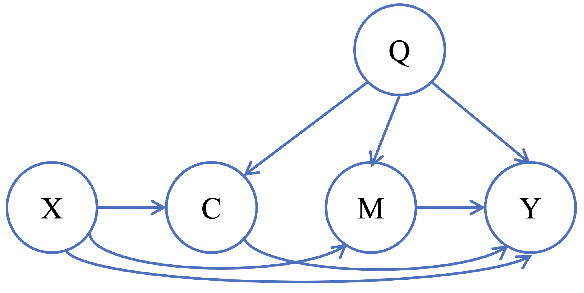
As an illustration of the significance of the path-specific effect, consider the structural causal model (SCM) in Figure 1, which describes a hiring process based on an applicant’s gender, number of children, physical strength, and qualifications [7]. The effect of gender (X) on the hiring decision (Y) can be decomposed into three different pathways starting from X and ending in Y: the direct impact of gender (unfair) ${\pi }_1:X\to Y$; the impact mediated by the number of children ${\pi }_2:X\to C\to Y$ (unfair, as it also discriminates against women who have children); and the impact mediated by physical strength ${\pi }_3:X\to M\to Y$ (fair). It is essential to measure each path’s effect in the SCM to analyze the hiring process’ fairness. The importance of the path-specific effect is also demonstrated in other domains, such as protein signaling networks, which provide insight into how signaling molecules influence subsequent molecules in the cascade [2] and biological pathways of symptoms, where it elucidates the impact of a disease on symptoms [8]. Identifying and differentiating specific pathways can contribute to a deeper understanding of complex diseases and may lead to new insights into disease mechanisms.

However, using the classical definition of the path-specific effect [9] has limitations in assessing the fairness of SCM. This is because it only provides an average effect estimate at the population (type) level without considering individual-level impact (token). For example, the impact of gender on hiring $(X\to Y)$ can be very small on average for the population but it can be large for an individual.

To overcome this limitation, we present a novel definition of the causal counterfactual path-specific importance score at the individual level. The proposed definition has three major advantages. Firstly, it can quantify individual-level impact through a specific pathway from the source vertex to the target vertex. Secondly, for paths with multiple edges, the effect can be decomposed into individual edges and evaluated as the product of the effects associated with the edges, making it cognitively intuitive for humans to understand. Finally, the computation of the proposed definition is efficient compared to the classical path-specific effect calculation, which is computationally demanding due to the need to evaluate each path independently. In complex causal graphs where the number of pathways grows exponentially with the number of edges, evaluating all pathways from the source vertex to the target vertex can be expensive. Our proposed path-specific importance score has desirable mathematical properties and can be efficiently computed through our designed algorithm.

In summary, we defined a causal counterfactual path-specific importance score, which quantifies the individual-level impact of a specific path from the source variable to the target variable. We show that our metric has desirable mathematical properties, including adherence to chain rules and consistency. Additionally, we present an algorithm that can efficiently compute the scores of all paths from the source vertex to the target vertex and identify the k-most significant paths in a causal graph with the highest scores.

The structure of this paper is as follows. Section 2 introduces preliminary knowledge related to causality. Section 3 presents our definition of path-specific counterfactual importance score. In Section 4, we establish the mathematical properties of the importance score. In Section 5, we propose an efficient algorithm to identify the most important path. Section 6 provides the evaluation of our method, while Section 7 presents related works in the field. Section 8 offers a detailed discussion of our findings. We summarize our work in Section 9. Lastly, the appendix provides proof of theorems and lemmas.

2. Preliminaries

We introduce the notation used to express concepts and variables. Capital letters, such as X, are utilized to represent random variables, while small letters, such as x, are utilized to denote the realizations of these variables. Bold letters, such as $\mathbf{X}$, are used to denote vectors of random variables. Calligraphic letters, such as $\mathcal{X}$, are used to represent sets. For a given natural number n, the $\left[n\right]$ is defined as the set $\{1,2,\cdots ,n\}$.

2.1. Causal Graph and Skeleton

Causal graphs are probabilistic graphical models specifically constructed to depict data-generating processes  [10]. In the graph, each vertex represents a variable. With a given variable set denoted as $\mathcal{V}=\{V_i,i\in \left[n\right]\}$, a directed edge started from variable $V_j$ and ended with $V_i$ implies that $V_i$ reacts to modifications in $V_j$, with all other variables in the causal graph maintaining respective constant values. Direct causes of $V_i$, or its parent variables, are defined as those linked to $V_i$ through directed edges, denoted by the set $\mathcal{P}{a}_i$. The underlying structure of a causal graph, commonly referred to as its skeleton, is determined by the graph’s overall topology.

2.2. Structural Causal Models (SCM)

The Structural Causal Model (SCM) introduces a framework in which the value of each variable $V_i$ can be determined as a function of both its parent variables and exogenous variables within a causal graph. This formalization proceeds as follows: let $\mathcal{V}=\{V_i,i\in \left[n\right]\}$ denote a set of endogenous (observed) variables, and let $\mathcal{U}=\{U_i,i\in \left[n\right]\}$ stand for a set of exogenous (unobserved) variables. An SCM is then established through a series of structural equations [10]:

$$V_i=f_i(\mathcal{P}{a}_i,U_i),\mathcal{P}{a}_i\subset \mathcal{V},U_i\subset \mathcal{U},i\in \left[n\right],$$

(1)

where function $f_i$ signifies the causal mechanism of $V_i$, thereby determining the value of $V_i$ contingent upon its parent variables and the respective exogenous variables.

2.3. Intervention and Do-Operation

The intervention of a variable on an SCM, denoted by the $do(·)$ operator, refers to assigning a constant value v to $V_i$, irrespective of its structural equation in the SCM. $do(V_i=v)$ means setting the value of $V_i$ to a constant v regardless of its structural equation in the SCM, i.e., ignoring the edges into the vertex $V_i$. This equates to disregarding the edges leading into the vertex $V_i$ in the causal graph. After intervention $do(X=x)$, the distribution of Y is denoted by $P(Y_{X=x}=y)$, where the variable $Y_{X=x}$ is the value of Y after intervention $do(X=x)$.

2.4. Path

Given a graph G, a path from vertex X to vertex Y in G is a finite sequence of edges $\pi$ that originates at X and terminates at Y, such that any two consecutive edges in $\pi$ are adjacent and all vertices are distinct. In particular, $\pi$ can be a direct edge $\left\{XY\right\}$ or a sequence of edges $\{X{V}_1,V_1{V}_2,\cdots ,V_{m-1}Y\}$.

2.5. Counterfactual Reasoning

Counterfactual reasoning enables the exploration of hypothetical “what if” scenarios. Consider a set of the endogenous (observed) variable $\mathcal{O}$ in the causal graph and an observation o referring to a realization of these variables, given $X=x$, the counterfactual question is asking what the potential outcome is if X were assigned a different value, $x^{\prime }$ [10]. The counterfactual outcome of Y is represented as $Y_{X=x^{\prime }}|X=x,\mathcal{O}=o$. With a given SCM, deterministic counterfactual reasoning can be accomplished through intervention as follows:

• Recover the exogenous variable value U as u, via the structural functions and the values $X=x$, $\mathcal{O}=o$;
• Calculate the counterfactual outcome $Y_{X=x^{\prime }}|U=u$. Specifically, within the SCM, assign the value of X to $x^{\prime }$ and substitute all exogenous variable values U as u on the right side of each structural function to obtain the value of Y.

The two steps are called deterministic counterfactual reasoning  [11], because the value of U can be solved uniquely from f when X and o are given. If the exogenous variable U in step 1 has multiple solutions, then nondeterminism should be involved in causal models by assigning a prior probability $P(U=u)$. In the nondeterministic counterfactual reasoning [11], step 1 is to update $P\left(U\right)$ as $P\left(U\right|X=x,\mathcal{O}=o)$, and the counterfactual outcome in step 2 is defined as the expectation over the posterior distribution of U.

3. Causal Effect along Different Pathways

We consider an SCM that represents the causal relationships among a set of variables $\mathcal{V}=\{V_i,i\in \left[n\right]\}$ that are given. All structural functions $f_i,i\in \left[n\right]$ are assumed to be continuous, with bounded derivatives on their respective domains. Additionally, we assume the corresponding causal graph G is a directed acyclic graph (DAG), as an example depicted in Figure 1.

Our primary objective is to examine the influence of a source vertex X on a target vertex Y, where $X,Y\in \mathcal{V}$. The most prevalent definition of a causal effect is applied within the medical field for binary cases, where the outcome variable Y depends on whether a patient accepts the diagnosis D or not. In this context, the causal effect is defined as the expected difference between these two scenarios within the population, denoted by $\mathbb{E}\left[Y_{D=1}\right]-\mathbb{E}\left[Y_{D=0}\right]$. Building upon this concept, to evaluate the causal effect at an individual level, allowing the algorithm to quantify the impact for a specific data point, we introduce the total counterfactual importance score described in Definition 1. This method incorporates counterfactual reasoning and a perturbation value $\delta$ in the denominator of Equation  (2).

Definition 1.

(Total Counterfactual Importance Score) Given a factual observation $o:\{V_i=v_i|i=1,\dots ,n\}$, which is a realization of all endogenous variables, for $\forall X,Y\in \mathcal{V}$, the counterfactual importance score of X on Y when $\mathcal{O}=o$ is

$$w_{X\to Y|o}=\underset{\delta \to 0}{lim}\frac{\mathbb{E}\left[Y_{X=x+\delta }\right|o]-\mathbb{E}\left[Y_{X=x}\right|o]}{\delta },$$

(2)

where $X=x$ is the factual observation from o.

The numerator represents the difference between two counterfactual outcomes of Y in the situations X is setup to X or $x+\delta$ when given the observation o. By incorporating the denominator $\delta$ and the limit operation in Equation (2), this definition intuitively captures how Y responds to the change on X given the current observation o. A larger value of effect scores for a path indicates greater significance for that path.

Next, we will discuss how to perform an intervention on a variable along a path. Furthermore, we introduce the concept of the path-specific counterfactual importance score for a given path $\pi$, which starts from variable X and ends at variable Y. This score quantifies the causal effect from the source variable to the target variable along a specific path. A direct edge can be considered a special case of a path.

Definition 2.

(Intervention on a variable along a path) For an SCM M, given a path (or an edge, a subgraph) π, we can partition each vertex $V_i$ ’s parents into two parts $P{a}_i=P{a}_i\left(\pi \right)\cup P{a}_i\left(\tilde{\pi }\right)$, where $P{a}_i\left(\pi \right)$ represents those members of $P{a}_i$ that are linked to $V_i$ in π and $P{a}_i\left(\tilde{\pi }\right)$ represents the complementary set. The operation of intervention of $X=x$ on the path π is defined as: we replace the structural equation $f_i$ as $f_i{(P{a}_i,u)}^{\pi }=f_i(P{a}_i{\left(\pi \right)}_{X=x},P{a}_i\left(\tilde{\pi }\right),u)$, where $P{a}_i{\left(\pi \right)}_{X=x}$ represents it taking the value when $X=x$ is enforced. The outcome of Y after the intervention of $X=x$ on the path π can be represented as $Y_{X=x\left(\pi \right)}$, where $x\left(\pi \right)$ represents value x in the path π.

Definition 3.

(Path-Specific Counterfactual Importance Score) Given a factual observation $o:\{V_i=v_i|i=1,\dots ,n\}$, which is a realization of all endogenous variables, and a causal path π in graph G, the path-specific counterfactual importance score of source vertex X on target vertex Y along path π is defined as follows:

$$w_{X\stackrel{\pi }{\to }Y|o}=\underset{\delta \to 0}{lim}\frac{\mathbb{E}\left[Y_{X=x+\delta \left(\pi \right),X=x\left(\tilde{\pi }\right)}\right|o]-\mathbb{E}\left[Y_{X=x}\right|o]}{\delta }.$$

(3)

Here, $X=x$ is the factual observation. The term $\tilde{\pi }={\mathsf{\Pi }}_{X\to Y}\setminus \pi$ represents the set of all paths from X to Y excluding path π, where ${\mathsf{\Pi }}_{X\to Y}$ is the set of all paths from X to Y. When the path is a direct edge from X to Y, the notation $w_{X\stackrel{\pi }{\to }Y|o}$ can be simplified as $w_{l_{XY}|o}$. The first term in the numerator represents the counterfactual outcome of Y when X is fixed at $x+\delta$ if X is part of path π; otherwise, it remains fixed at x.

The numerator captures the effect of X on Y through the given $\pi$. Definition 3 can quantify how Y responds to the change on X only through a path $\pi$ given the current observation o. In our model, the direct effect is defined as the effect propagated only through the edge directly connecting the source and target, which can be regarded as a special case of path-specific effect.

Intuitively, Definition 3 uses the intervention operation on a path and only considers the effect of the changing of X on Y propagating from the given path $\pi$. We will keep X as its original value for other edges in the graph. Intuitively, if the change caused by the intervention is larger, the causal strength of X to Y on these paths is larger. The operation of intervention on a path isolates the impact on Y by X on the given path. The normalization and limitation operation on the intervention value provides some “independence” among edges of the causal effect in a path. These exhibit desirable properties.

The numerator is similar to the definition of the counterfactual path-specific effect in [5]. However, they focus on the discrete case. Although [5] can be directly extended to the individual level, it does not have the math properties we propose in the next section. Our definition adds the normalization of the intervention value in the denominator and focuses on the strength of the local effect by limitation operation. Intuitively, these modifications provide some “independence” of the causal effect in the graph. So, our method has more straightforward decomposition and fast calculation properties (discussed in the next section), which are important for explaining and evaluating the causal effect along each path.

The limit format of the perturbation value $\delta$ has a similar format to that of the incremental causal effect and the marginal treatment effect [12,13,14]. Ours are defined on the counterfactual reasoning and the path-specific effect. However, they focus on the total or direct effect.

4. Properties of Path-Specific Counterfactual Importance Score

As previously stated in the introduction, the traditional definition of the path-specific effect encounters difficulties in decomposing its effect to individual edges and computing it efficiently. This section delves into the mathematical properties of our path-specific counterfactual importance score, which addresses these limitations.

In detail, we discuss the connection between our definition and the partial derivative involved in the calculation, as well as the consistency between the total importance score and path-specific score. First, we introduce an assumption and a lemma pertinent to the direct effect, which refers to an edge that directly connects the source and target vertex within the graph.

Lemma 1.

For an SCM M, given an edge from X to Y, and the structural causal equation of Y: $Y=f_Y(X,{\mathbf{Z}}_{\mathbf{yx}},U_y)$, where ${\mathbf{Z}}_{\mathbf{yx}}$ represents all parents of Y excluding X. Given a factual observation o, the counterfactual importance score of X on Y along the path/link $\pi =l_{XY}=\left\{XY\right\}$ is the partial derivative of Y with respect to X at the point of the observation. Formally,

$$\begin{array}{cc}\hfill w_{l_{XY}|o}& ={\mathbb{E}}_{U_y|o}\left[{\left.\frac{\partial Y}{\partial X}\right|}_o\right]\hfill \\ \hfill & ={\mathbb{E}}_{U_y|o}\left[{\left.\frac{\partial Y}{\partial X}\right|}_{X=x,{\mathbf{Z}}_{\mathbf{yx}}={\mathbf{z}}_{\mathbf{yx}},U_y=u_y}\right]\hfill \\ \hfill & =\int {\left.\frac{\partial Y}{\partial X}\right|}_{X=x,{\mathbf{Z}}_{\mathbf{yx}}={\mathbf{z}}_{\mathbf{yx}},U_y=u_y}P\left(u_y\right|o)d{u}_y.\hfill \end{array}$$

(4)

Lemma 1 does not require the exogenous variables $\mathcal{U}$ to be deterministically recovered (having a unique solution when $f,X,o$ are given). The derivation is based on nondeterministic counterfactual reasoning. It shows that the value of the path-specific counterfactual importance score in an edge case is the partial derivative of Y concerning X in the counterfactual reasoning data point weighted by the posterior probability of $\mathcal{U}$. Additionally, if exogenous variables $\mathcal{U}$ can be perfectly recovered as $\mathbf{u}$, given a factual observation $o:\{V_j=v_j|j=1,\dots ,n\}$, then Equation (4) in Lemma 1 can be simplified as Equation (5). The detailed proof of Lemma 1 can be found in Appendix A.

$$w_{l_{XY}|o}={\left.\frac{\partial Y}{\partial X}\right|}_o.$$

(5)

We introduce the following assumption about exogenous variables $\mathcal{U}$.

Assumption 1.

(Independent exogenous variables assumption) All exogenous variables $\mathcal{U}$ are independent.

Based on Lemma 1, when Assumption 1 holds true, we can derive the following theorem for a general path in the causal graph, which shows that the calculation of the importance score for each edge in the graph is independent and the importance score for a path is the multiplication of the importance score for each edge inside the path. Our path-specific score can be directly decomposed to individual edges. This is helpful for understanding the effect of these edges on the outcome and designing effective algorithms for calculating the importance score in the graph. The detailed proof of Theorem 1 is in Appendix A.

Theorem 1.

(Chain rule: path-specific counterfactual importance score and partial derivative). For an SCM M, when Assumption 1 holds true, given a path $\pi =\{X{V}_1,V_1{V}_2,\cdots V_{m-2}{V}_{m-1},$$V_{m-1}Y\}$ with length m and a factual observation o, the path-specific counterfactual importance score of the source vertex X on target vertex Y along the path π can be represented as:

$$\begin{array}{cc}\hfill w_{X\stackrel{\pi }{\to }Y|o}& =w_{l_{X{V}_1}|o}\left(\prod _{i=1}^{m-2}{w}_{l_{V_i{V}_{i+1}}|o}\right)w_{l_{V_{m-1}}Y|o}\hfill \\ \hfill & =\left.{\mathbb{E}}_{U_1|o}{\left[\frac{\partial V_1}{\partial X}\right|}_o\right]\left(\prod _{i=1}^{m-2}{\mathbb{E}}_{U_{i+1}|o}\left[{\left.\frac{\partial V_{i+1}}{\partial V_i}\right|}_o\right]\right)\hfill \\ \hfill & \left.{\mathbb{E}}_{U_Y|o}{\left[\frac{\partial Y}{\partial V_Y}\right|}_o\right].\hfill \end{array}$$

We also show the consistency of our definition in Theorem 2. The sum of counterfactual path-specific scores among all paths from source to target is the same as the total counterfactual importance score from source to target. It provides the connection between Definitions 1 and 3. This makes the addition and comparison among different paths’ scores more meaningful. The detailed proof is in Appendix A.

Theorem 2.

(Consistency) Given an SCM M and a factual observation o, when Assumption 1 holds true, the total counterfactual importance score of X on Y equals the summation of path-specific counterfactual importance score among all the possible paths from X to Y:

$$w_{X\to Y|o}=\sum _{\pi \in {\mathsf{\Pi }}_{X\to Y}}{w}_{X\stackrel{\pi }{\to }Y|o}.$$

5. Efficient Algorithm for the Most Important Path

In reality, given an SCM, people are more interested in finding the most important path that has the largest impact. We define the most important paths from the source to the target as the path with the largest absolute value of the Importance score. We introduce Algorithm 1 to find the most important path effectively. We note that this algorithm can be easily extended to the k-most important path, by using a priority queue.

Algorithm 1 Fast calculation for the most important path.

1: Inputs: Graph G(V, E), source vertex X, target vertex Y 2: Outputs: Path P 3: Calculate the path-specific importance score for each edge in the graph: $w_1,w_2,\cdots ,w_n$, where $n=\left|E\right|$ 4: Transfer the importance score to log scale, $log\left(\right|w_1\left|\right),log\left(\right|w_2\left|\right),\cdots ,log\left(\right|w_n\left|\right)$ 5: Define a graph $G^{\prime }$ that maintains same skeleton as graph G, with edge weight $log\left(\right|w_1\left|\right),log\left(\right|w_2\left|\right),\cdots ,log\left(\right|w_n\left|\right)$ 6: Path P = LongestPathDAG($G^{\prime }$, X, Y) 7: return P

Based on Theorem 1, the calculation for the importance score for each edge is independent. So, we can evaluate each edge’s score first and then calculate the path’s score. Then, we notice that finding the most important path in the original causal graph can be reduced into finding the longest path in a DAG with different edge weights. In detail, based on Theorem 1, the importance score for a path is the multiplication of the importance score for each edge inside the path. We denote the importance score of all edges in a graph as $w_1,\cdots ,w_n$, where n is the number of edges. Because of the monotonicity of the log function, ${\prod }_{i=1}^n\left|w_i\right|$ achieves the largest value as the $log\left({\prod }_{i=1}^n\right|w_i\left|\right)$. Then, we can transfer it from the multiplication to the summation as follows:

$$log(\prod _{i=1}^n|w_i\left|\right)=\sum _{i=1}^{n}log\left(\right|w_i\left|\right).$$

Next, we define a new graph $G^{\prime }$ with the same skeleton as the original graph G, but the length for edge i is $log\left(\right|w_i\left|\right)$, rather than $w_i$, $i\in \left[n\right]$. For each path in $G^{\prime }$ with a length of ${\sum }_{i=1}^{n}log\left(\right|w_i\left|\right)$, there exists a corresponding path in G with an absolute importance score of ${\prod }_{i=1}^n\left|w_i\right|$. Given the monotonicity of logarithms, the most important path in the original graph G corresponds to the longest path in the transformed graph $G^{\prime }$. Finally, Algorithm 1 calls a subroutine Algorithm 2 to calculate the longest path in a DAG [15]. Because of the acyclic property, Algorithm 2 can find the longest path in polynomial time by topological sort and dynamic programming.

Algorithm 2 Longest path in DAG.

1: Inputs:Weighted DAG graph $G(V,E)$, source vertex X, target vertex Y 2: Outputs: Path P 3: Linearized order $\mathcal{V}$ = Topologically sort G 4: for each vertex $v\in \mathcal{V}$ in linearized order from X to Y do 5:    $dist\left(v\right)={max}_{u,v\in E}(dist\left(u\right)+w(u,v)$) 6:    $v_{previous}=argma{x}_{u,v\in E}(dist\left(u\right)+w(u,v)$) 7: end for 8: Recursively find the path using $v_{previous}$ starting from X to Y 9: return P

Our methodology retains its applicability even when $|w_i|$ is less than 1. If $|w_i|$ is found within the range of 0 to 1, then the associated edge length $log\left(\right|w_i\left|\right)$ in the graph $G^{\prime }$ is a negative value. As we presuppose the causal graph to be acyclic, issues related to negative cycles are avoided and the validity of our longest path computation is preserved. Intuitively, when $|w_i|$ lies between 0 and 1, in the original graph G, the expansion of a path by an edge results in a decrease in the path’s importance score. Correspondingly, in the graph $G^{\prime }$, a negative path $log\left(\right|w_i\left|\right)$ contributes to a decrease in path length. Consequently, the consistent correlation between these observations validates our approach.

The time complexity of Algorithm 1 is in the linear scale of number of edges and vertices, $O\left(\right|E|+|V\left|\right)$ [16]. Compared with the case using the classical definition, where the calculations for each path are independent, and the number of paths is exponential to the edge, our algorithm significantly improves finding the most important path in the causal graph.

Because of the math property that the edge’s scores are independent, we can easily formulate our definition of the path-specific score into the existing algorithm that is based on a graph theorem to design an efficient algorithm. For example, we can use the algorithm in [17] to find the paths with the top k largest importance score in a causal graph.

6. Evaluation

We demonstrate the performance of our method for path-specific analysis using two datasets, one synthetic and the other real.

6.1. Job Hiring Problem

We assume the following SCM for the physically demanding job hiring process discussed in the introduction (illustrated in Figure 1):

$$\begin{array}{cc}\hfill X& =U_x,U_x\sim Bernoulli\left(0.6\right)\hfill \\ \hfill Q& =U_Q,U_Q\sim \mathcal{N}(2,5^2)\hfill \\ \hfill C& =X+0.5Q{U}_c,U_c\sim Tr\mathcal{N}(2,1^2,0.1,3.0)\hfill \\ \hfill M& =3X+0.4Q{U}_M,U_M\sim Tr\mathcal{N}(3,2^2,0.1,3.0)\hfill \\ \hfill Y& =h(X,Q,C,M)=\zeta (-10+5X+C+Q+M),\hfill \end{array}$$

where $Bernoulli$, $\mathcal{N}$, and Tr$\mathcal{N}$ represent the Bernoulli, Gaussian, and truncated Gaussian distributions, respectively, and $\zeta \left(k\right)=1/(1+exp(-k\left)\right)$ denotes the standard sigmoid function. A similar data generation process was employed in [7].

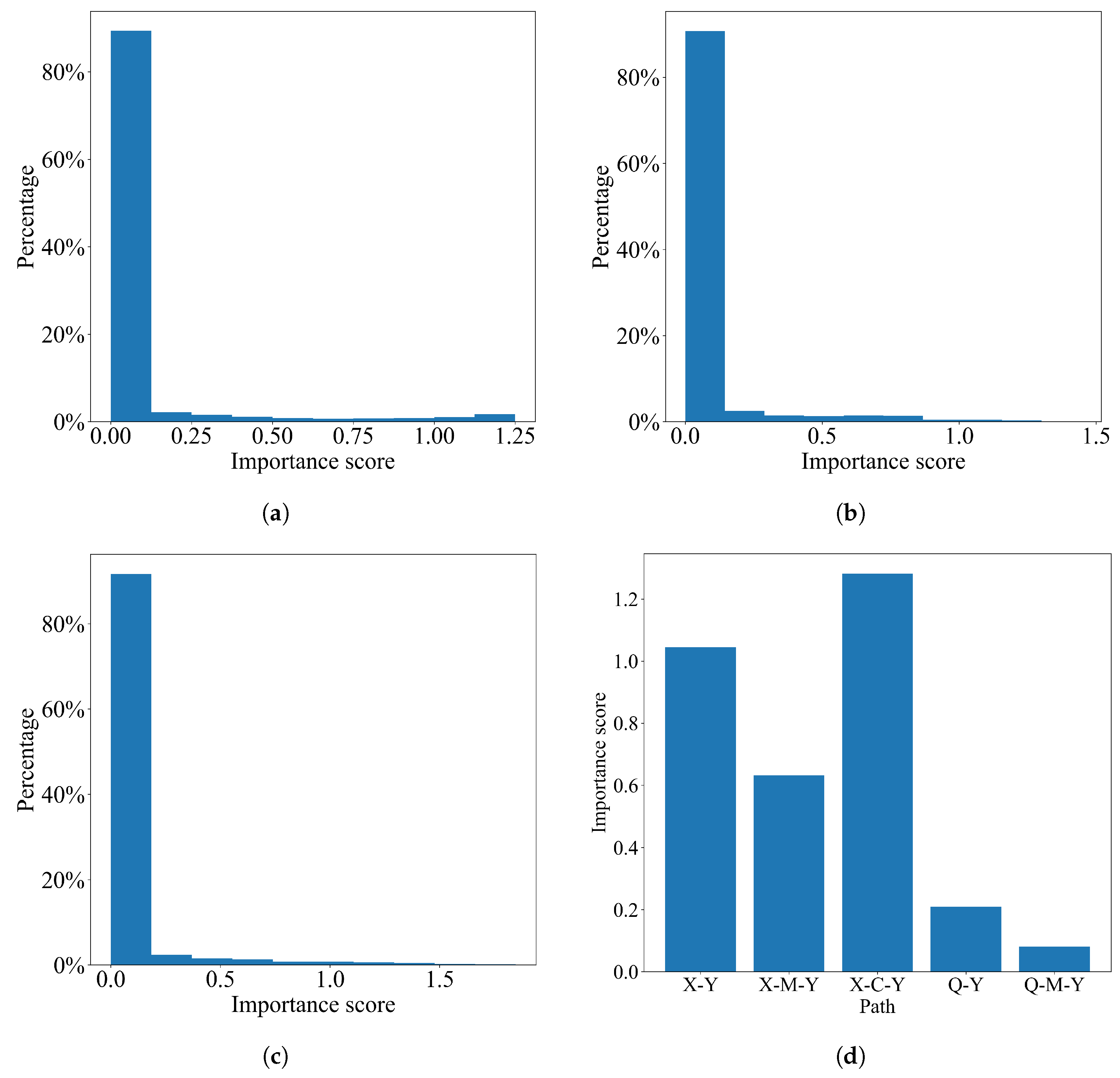
The simulation results are presented in Figure 2. The first three figures display population-level results. Specifically, they illustrate the distribution of importance scores for three distinct paths, originating from gender and ending in hiring, which quantify the impact of X on Y. For the majority of individuals (over $80\%$), the effect of these three paths is small, indicating that the model appears fair on average. This result aligns with the classical definition at the population level.

In the final subfigure, we examine a specific individual and assess the impact of all paths related to hiring decisions of Figure 1 for this particular individual. We observe that the hiring process is unfair for this individual, as the impact of the unfair paths $X\to Y$ and $X\to C\to Y$ possess importance scores comparable to other paths. This example highlights how our approach can be utilized to quantify the influence of paths for individuals.

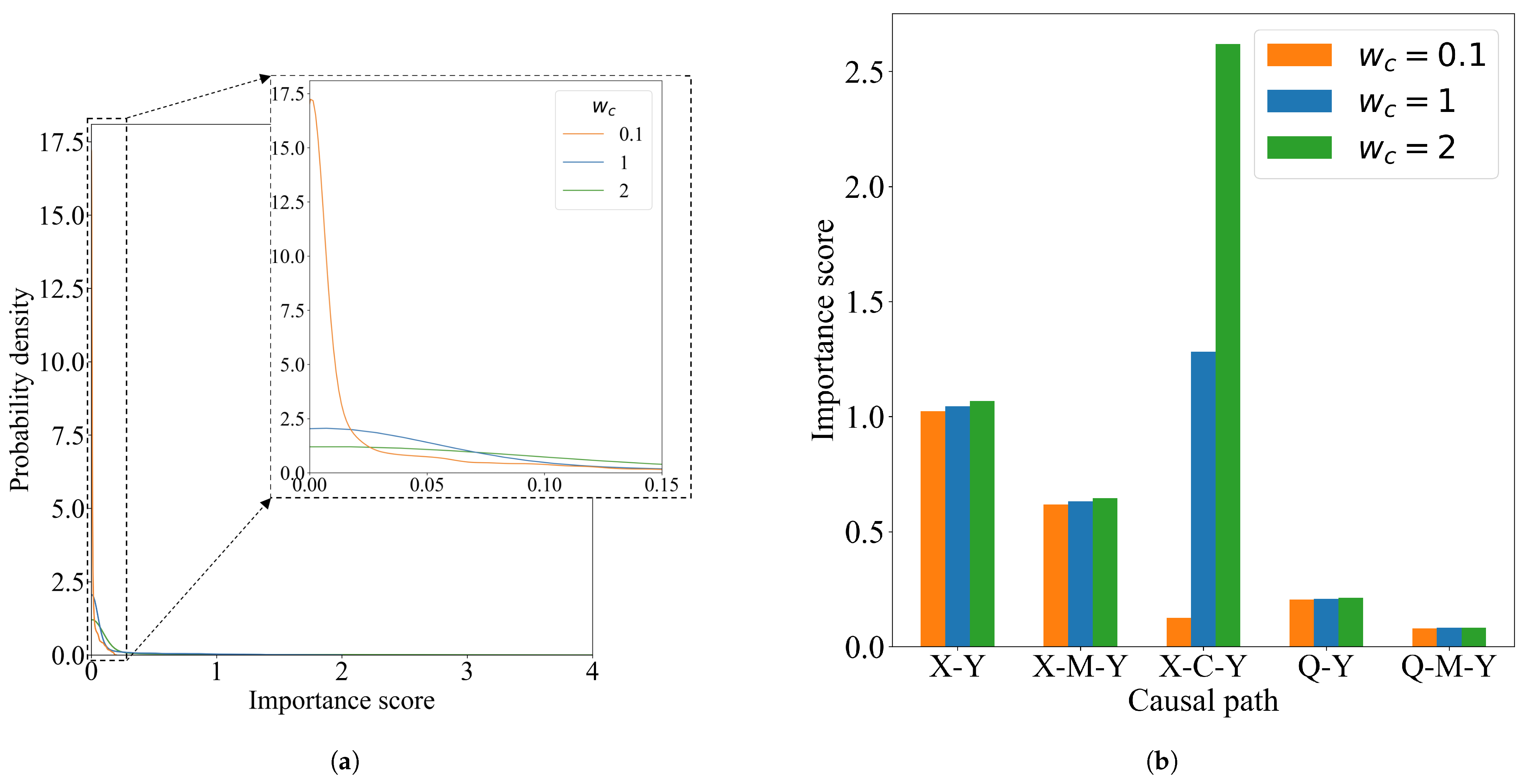
To further investigate the variations in importance scores for paths within the population and at the individual level, we introduce a weight coefficient, $w_c$, corresponding to the ‘number of children’ feature, into the equation for Y. An increase in the value of $w_c$ signifies an amplified impact of feature C on Y.

$$Y=h(X,Q,C,M)=\zeta (-10+5X+w_{c}C+Q+M).$$

Our analysis results are depicted in Figure 3. The first figure presents the distribution of importance scores for path $X-C-Y$. The second figure relates to the individual-level importance scores. We note that, as the value of $w_c$ increases, the importance score for path $X-C-Y$ increases correspondingly, while the scores for other paths remain almost unchanged. This indicates an increased level of unfairness associated with this specific path, in line with the changes in $w_c$.

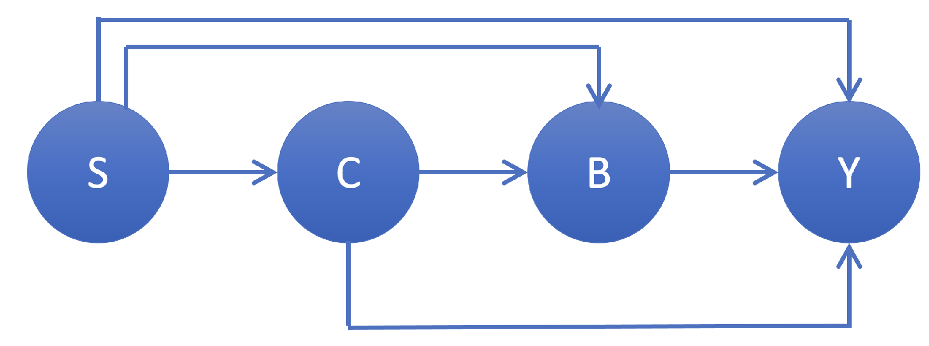
6.2. Smoking Impact Problem

We also evaluated our method using a real dataset—the Framingham Heart Study dataset [18]. The original Framingham cohort dataset comprises two years of examination data for 5209 participants aged between 30 and 62 years. Our objective was to investigate the causal mechanisms of smoking behavior on systolic blood pressure (SBP) mediated by cholesterol levels and body weight (depicted in Figure 4). Our SCM was formulated as a linear regression model with some covariant terms, as recommended by [19].

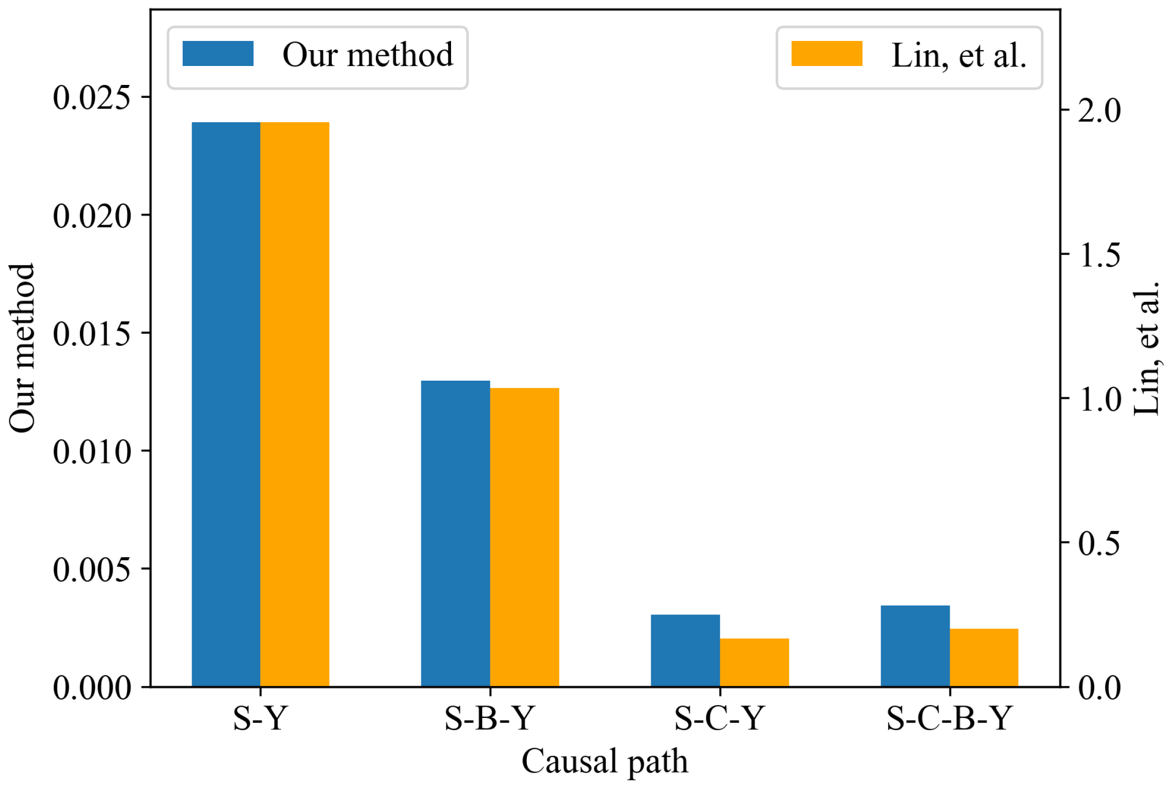
Figure 5 presents the average effect of the paths that begin with smoking and end with SBP at the population level by using our method. Our method reveals that the direct impact of smoking on blood pressure, denoted as ($S\to Y$), has the highest average importance score in comparison with the other three paths. Consequently, the direct path’s influence is the most dominant factor relative to other paths. Notably, the ranking for the paths sorted by their importance based on our method is consistent with the conclusion drawn in [19]. We believe the difference in the magnitude of the results is due to the different perturbation values used by the two methods.

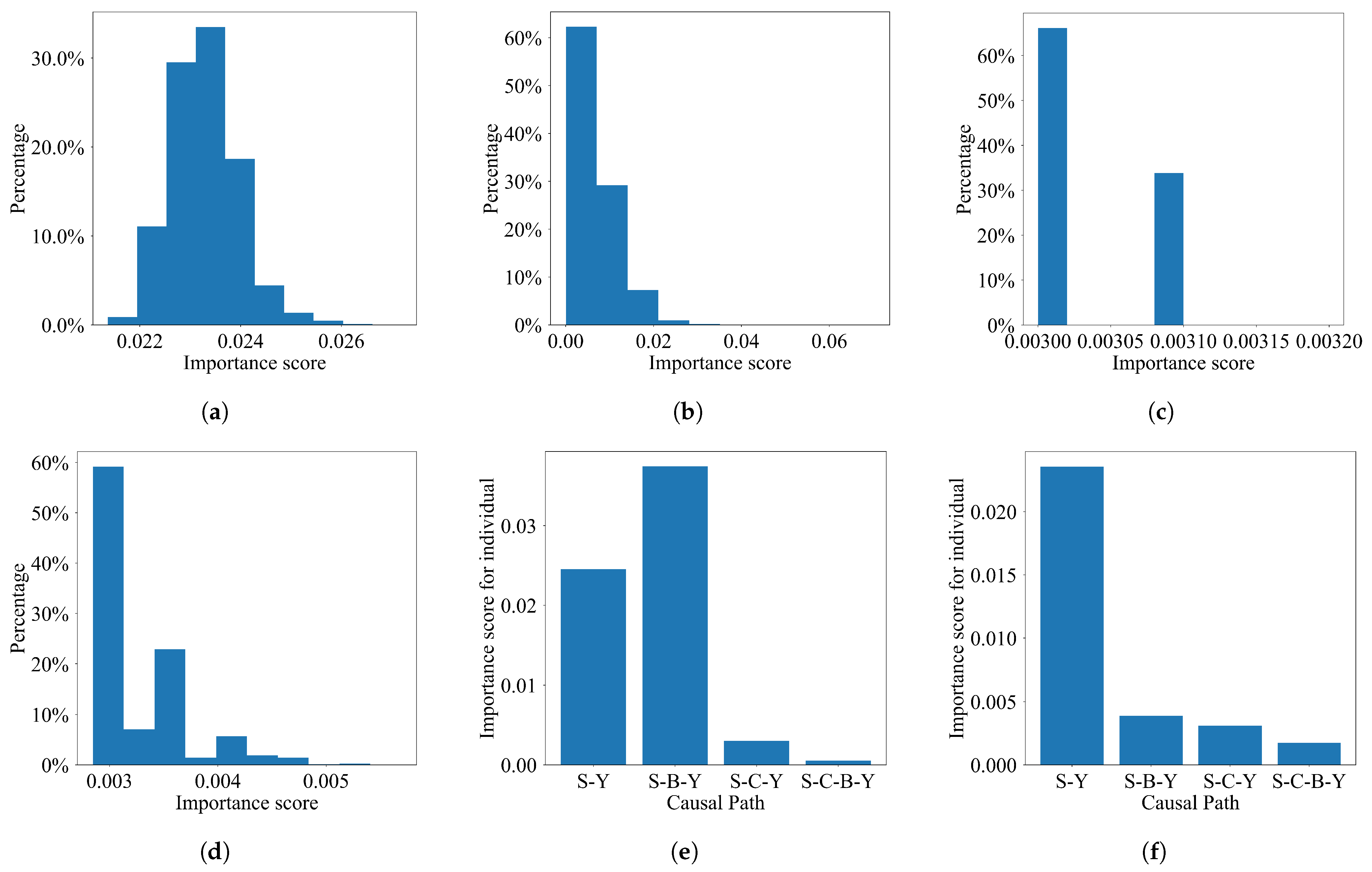
The first four subfigures of Figure 6 display the distribution of importance scores along the paths that begin with smoking and end with SBP at the population level. Additionally, the last two subfigures show the individual-level importance of these paths for two specific individuals. Interestingly, we find that, for person A, both the direct path from smoking to blood pressure ($S\to Y$) and the path of smoking affecting blood pressure through body weight ($S\to B\to Y$) are significant. However, for person B, the direct impact of smoking on blood pressure ($S\to Y$) is the dominant factor. This type of individual-level path analysis provided by our method can help an individual know each path’s influence for the particular individual.

7. Related Works

The study of path-specific analysis has garnered significant interest within the academic community. A majority of the existing research has centered around non-parametric settings, identifiability, or informational decomposition of SCMs [20,21,22]. These approaches diverge from our work, which is grounded in a known SCM model. Our method enables the quantification of individual-level path-specific effects and the development of efficient algorithms to identify the most crucial paths.

Several related studies have proposed causal effect definitions such as incremental causal effects and marginal treatment effects [12,13,14]. These definitions employ a similar constraint format for the perturbation value $\delta$. However, while their focus lies on total effects and population-level analysis, our work concentrates on path-specific effects and offers individual-level quantification.

We elucidate the relationship between our work and existing literature concerning population-level causal effects. In particular, the studies by Janzing et al. [23] and Wang et al. [24] both define and measure causal strength (effect) using Shapley values. Janzing et al. [25] assess causal influence based on the distributional change resulting from removing a “causal arrow”. Furthermore, Janzing’s concept of intrinsic causal contribution [23] allows for the separation of intrinsic information added by each vertex from the information obtained from its ancestors. Wang et al. [24] allocate credit to edges and provide an interpretation of the entire causal graph. In contrast, our method builds upon the classical definition of average treatment effect, which is grounded in intervention operations, and extends this definition to continuous and individual cases. Our approach boasts advantages such as the clear decomposition of causal effects along paths and rapid calculations for identifying the most important paths. This transparent decomposition proves critical for interpreting the entirety of the SCM.

8. Discussions

8.1. Motivation for Path-Specific Effects

In certain applications, the analysis of path effects yields vital information that is not captured by total effects. Notable examples include the fairness analysis of a model as discussed in the introduction, protein signaling networks (which examine the influence of signaling molecules on subsequent molecules within the cascade) [2], and the biological pathway of symptoms (exploring the impact of a disease on its symptoms) [8]. Identifying and distinguishing specific pathways can enhance our understanding of complex diseases and potentially offer novel insights into disease mechanisms.

8.2. Linear Case

Based on our definition, when all structural equations are linear, the individual-level effect is equivalent to the population-level effect, as the difference between the counterfactual after perturbation and the original is independent of $\mathcal{U}$. Consequently, for each edge, the path-specific score is the partial derivative of the structural function, which corresponds to the coefficient of the linear function. Simultaneously, using Theorem 1, the path-specific score for a given path is determined by the product of each variable’s coefficient within its respective linear model along that path.

8.3. Assumptions

We do not make the assumption that $\mathcal{U}$ is perfectly recovered, which is only necessary for deterministic counterfactual reasoning and facilitates the calculation of the expectation over $\mathcal{U}$. The only requirement is the independence of $\mathcal{U}$ (Assumption 1). Without perfectly recovered $\mathcal{U}$, our definitions and theorems remain valid, and our method can still be employed based on nondeterministic counterfactual reasoning, as evidenced by our experiments.

8.4. Single-Point Derivatives and Potential for Severe Errors

Our objective was to quantify the local effect at a specific point; hence, we used a method that concentrates on a single point to preserve generality. We recognized that the product of effects along a causal path may lead to error propagation and amplification, a common issue when estimating a path’s strength. This arises because the target vertex can be represented as a multi-layer composition function of the source vertex through the causal graph structure. We intend to explore this challenge in future work.

9. Conclusions

In this study, we presented a novel metric for path-specific effect analysis, termed the causal counterfactual path-specific importance score. This score quantifies path-specific effects at the individual level. We demonstrated that our metric exhibits desirable mathematical properties, such as compliance with chain rules and preservation of consistency. These properties facilitate the decomposition of the path-specific score into each edge within the path, enabling the development of an efficient algorithm to identify the most critical path in a causal graph in linear time with respect to the number of edges. Our simulations indicate that our innovative definition concurs with the classical definition at the population (type) level while also delineating path-specific effects at the individual (token) level.

References

- Baron, R.M.; Kenny, D.A. The moderator–mediator variable distinction in social psychological research: Conceptual, strategic, and statistical considerations. J. Personal. Soc. Psychol. 1986, 51, 1173. [Google Scholar] [CrossRef] [PubMed]
- Sachs, K.; Perez, O.; Pe’er, D.; Lauffenburger, D.A.; Nolan, G.P. Causal protein-signaling networks derived from multiparameter single-cell data. Science 2005, 308, 523–529. [Google Scholar] [CrossRef] [PubMed]
- Stock, J.H.; Watson, M.W. Identification and estimation of dynamic causal effects in macroeconomics using external instruments. Econ. J. 2018, 128, 917–948. [Google Scholar] [CrossRef]
- Chiappa, S. Path-specific counterfactual fairness. In Proceedings of the AAAI Conference on Artificial Intelligence, Honolulu, HI, USA, 27 January–1 February 2019; Volume 33, pp. 7801–7808. [Google Scholar]
- Wu, Y.; Zhang, L.; Wu, X.; Tong, H. PC-fairness: A unified framework for measuring causality-based fairness. Adv. Neural Inf. Process. Syst. 2019, 32, 3399–3409. [Google Scholar]
- Wang, X.; Meng, F.; Liu, X.; Kong, Z.; Chen, X. Causal explanation for reinforcement learning: Quantifying state and temporal importance. Appl. Intell. 2023. [Google Scholar] [CrossRef]
- Chikahara, Y.; Sakaue, S.; Fujino, A.; Kashima, H. Learning individually fair classifier with path-specific causal-effect constraint. In Proceedings of the International Conference on Artificial Intelligence and Statistics, PMLR, Online, 13–15 April 2021; pp. 145–153. [Google Scholar]
- Li, H.; Geng, Z.; Sun, X.; Yu, Y.; Xue, F. A novel path-specific effect statistic for identifying the differential specific paths in systems epidemiology. BMC Genet. 2020, 21, 85. [Google Scholar] [CrossRef] [PubMed]
- Avin, C.; Shpitser, I.; Pearl, J. Identifiability of Path-Specific Effects. In Proceedings of the 19th International Joint Conference on Artificial Intelligence, Edinburgh, Scotland, 30 July–5 August 2005; pp. 357–363. [Google Scholar]
- Pearl, J. Causality; Causality: Models, Reasoning, and Inference; Cambridge University Press: Cambridge, UK, 2009. [Google Scholar]
- Glymour, M.; Pearl, J.; Jewell, N.P. Causal Inference in Statistics: A Primer; John Wiley & Sons: Hoboken, NJ, USA, 2016. [Google Scholar]
- Rothenhäusler, D.; Yu, B. Incremental causal effects. arXiv 2019, arXiv:1907.13258. [Google Scholar]
- Zhou, X.; Xie, Y. Marginal treatment effects from a propensity score perspective. J. Political Econ. 2019, 127, 3070–3084. [Google Scholar] [CrossRef] [PubMed]
- Zhou, X.; Opacic, A. Marginal Interventional Effects. arXiv 2022, arXiv:2206.10717. [Google Scholar]
- Cormen, T.H.; Leiserson, C.E.; Rivest, R.L.; Stein, C. Introduction to Algorithms; MIT Press: Cambridge, MA, USA, 2022. [Google Scholar]
- Jungnickel, D.; Jungnickel, D. Graphs, Networks and Algorithms; Springer: Cham, Switzerland, 2005; Volume 3. [Google Scholar]
- Yen, S.H.; Du, D.H.C.; Ghanta, S. Efficient algorithms for extracting the k most critical paths in timing analysis. In Proceedings of the 26th ACM/IEEE Design Automation Conference, Las Vegas, NV, USA, 25–29 June 1989; IEEE: New York, NY, USA, 1989; pp. 649–654. [Google Scholar]
- Benjamin, E.J.; Levy, D.; Vaziri, S.M.; D’Agostino, R.B.; Belanger, A.J.; Wolf, P.A. Independent risk factors for atrial fibrillation in a population-based cohort: The Framingham Heart Study. JAMA 1994, 271, 840–844. [Google Scholar] [CrossRef] [PubMed]
- Lin, S.H.; VanderWeele, T. Interventional approach for path-specific effects. J. Causal Inference 2017, 5, 20150027. [Google Scholar] [CrossRef]
- Malinsky, D.; Shpitser, I.; Richardson, T. A potential outcomes calculus for identifying conditional path-specific effects. In Proceedings of the 22nd International Conference on Artificial Intelligence and Statistics, Naha, Japan, 16–18 April 2019; PMLR: London, UK, 2019; pp. 3080–3088. [Google Scholar]
- Zhang, J.; Bareinboim, E. Non-parametric path analysis in structural causal models. In Proceedings of the 34th Conference on Uncertainty in Artificial Intelligence, Monterey, CA, USA, 6–10 August 2018. [Google Scholar]
- Gong, H.; Zhu, K. Path-specific Effects Based on Information Accounts of Causality. arXiv 2021, arXiv:2106.03178. [Google Scholar]
- Janzing, D.; Blöbaum, P.; Minorics, L.; Faller, P. Quantifying causal contributions via structure preserving interventions. arXiv 2020, arXiv:2007.00714. [Google Scholar]
- Wang, J.; Wiens, J.; Lundberg, S. Shapley flow: A graph-based approach to interpreting model predictions. In Proceedings of the International Conference on Artificial Intelligence and Statistics, Valencia, Spain, 25–27 April 2021; PMLR: London, UK, 2021; pp. 721–729. [Google Scholar]
- Janzing, D.; Balduzzi, D.; Grosse-Wentrup, M.; Schölkopf, B. Quantifying causal influences. Ann. Statist. 2013, 41, 2324–2358. [Google Scholar] [CrossRef]
- Bartle, R. The Elements of Integration and Lebesgue Measure; Wiley Classics Library; Wiley: New York, NY, USA, 1995. [Google Scholar]