Developing a Numerical Method of Risk Management Taking into Account the Decision-Maker’s Subjective Attitude towards Multifactorial Risks

Abstract

Risk involves identifying several options that the decision-maker can opt for while making a choice either in the direction of risk or reliability. In this approach, risk is defined as the action of the subject which will lead to the loss or guaranteed safety of what has been achieved. As the uncertainty of the external business environment increases for companies, the task of managing risks both individually and as a set of risks becomes more and more relevant. The purpose of this study is to solve the problem of managing multifactorial risks using mathematical methods for determining the optimal risk management trajectories separately for each factor. To determine the optimal risk management trajectories for each factor, a numerical method is used based on the choice of the most effective direction, which is defined as the ratio of risk change to cost change. An information system prototype has been created that can support the management of a set of risks. Approbation of the information system was carried out on an example containing two conceptual risk factors. The proposed prototype builds a three-dimensional risk map by interpolating the risk matrix entered by the risk manager using an additive–multiplicative aggregation procedure, as well as optimal risk management trajectories for all entered risk factors.

1. Introduction

Science and practice have long established that in the world of economics and finance, risk is directly related to the applied management approaches and methods and is directly dependent on the effectiveness and validity of management decisions [1,2]. This can be seen as early as 1901, in A.H. Willett’s “The Economic Theory of Risk and Insurance”. Since then, the study of risks has only grown, and the search for the most effective ways to manage risks and prevent them has been continuous [3].

Correct decisions can reduce product costs, management costs, and eliminate potential problems that may adversely affect the company’s competitiveness.

Considering this, most researchers recognize that to maintain high competitiveness of companies in an actively changing global environment, it is necessary to strategically create effective risk management mechanisms in the short term [4]. Risk-oriented management in the company management system allows one to reduce the level of negative consequences from the occurrence of risky situations. At the same time, it has been proven that it is possible to manage the risks of an organization most effectively only if there is a unified planning and goal-setting system, which accordingly requires the use of modern methods of collecting and processing information, as well as the use of mathematical and digital methods for its analysis and processing. As a result, interest in various systemic risk management solutions has grown significantly.

Risk assessment is an integral part of the risk management mechanism [5]. It is used to analyze risks in terms of their likelihood of occurrence, determine the strength and depth of consequences, the possibility of their avoidance, as well as to make decisions on the elimination of consequences and develop further measures to reduce risks in the future. However, the risk management methods and tools used so far in many cases do not achieve the desired result and therefore expose companies to unaccounted risks.

The aim of this study is to solve the problem of managing multifactorial risks using numerical methods to determine the optimal risk management trajectories separately for each factor. Based on this, the following research hypothesis was formulated.

H1: 

The use of modern mathematical methods makes it possible to create a tool for managing multifactorial risks and optimize the costs of their management.

For investigating this research hypothesis, we create a computer program and formulate the problem of risk management as an optimization problem by minimizing the total cost of managing risk-forming parameters. Minimization problem has two constraints on risk-forming parameters falling into domain values and constraint that the combination of risk-forming parameters provides to a risk level calculated by risk function.

It should be noted that risk is understood as uncertainty associated with the danger of deviation from the goal, for the sake of which a subjective decision was made. We agree with the approach according to which risk is associated with the refraction of uncertainty through a subjective attitude to the consequences of the manifestation of uncertainty factors and the associated economic interests of a particular decision-maker [6].

The situation of risk involves the identification of several behaviors, during which one can make a choice in the direction of risk or reliability. In this approach, risk is defined as the action of the subject, which will lead to the loss or guaranteed safety of what has been achieved. As such, a properly constructed risk assessment and risk management system is of particular importance.

To formalize the attitude of the decision-maker to specific risks we suggest building a risk matrix. Risk matrix is built via crossing qualitative categories of risk-forming parameters and matching them to generated risk categories. In the next stage, the risk matrix is coded by numerical values. This makes it possible to approximate the risk function and to solve the above-formulated risk management problem. To approximate the risk matrix, it is proposed to use the continuous additive–multiplicative approach to aggregation.

2. Literature Review

The history of scientific and systematic study of risks, and the development of measures to protect from and prevent risks, and to reduce their negative consequences is more than a century old; the concept of risk management and assessment was first described in 1901 in the work of A.H. Willett titled “The Economic Theory of Risk and Insurance” [3]. Without dwelling on the history of the development of scientific thought in the field of risk management, in this section, we will highlight the current trends in the study of risks and the search for ways to prevent them.

In the modern literature, most often, risk is associated with the concept of competitiveness of companies (the danger of losing competitiveness under the influence of risks) and with the requirements for developing a strategy and mechanism for countering risks [7,8,9,10]. According to [4], sustainable management and development is an important requirement for the management strategy or business model of any enterprise since its absence will weaken competitiveness and make the long-term operation of the enterprise unlikely [4]. A sustainable management strategy allows a company to rise above its competition and change its position in social and environmental aspects, thereby increasing its competitiveness in the market [11]. Particularly, risk management in supply chains is extensively debated [12,13,14,15,16].

Research related to the combination of risk management and enterprise sustainability is gaining ground, such as [17,18,19], wherein it has been stated that a focus on social and environmental sustainability can help increase corporate trust among key stakeholders, which determines the needs of the market according to the economic, social, and environmental aspects, thereby enhancing and improving sustainable corporate performance and creating opportunities for sustainable management [19]. Many authors focus on the impact of corporate social responsibility on corporate risk [20,21,22].

A review of the scientific literature showed a huge variety of scientific schools, approaches, concepts, and risk management methods recommended for practical application in various types of companies [23,24,25,26].

Several studies have revealed a shift in emphasis in modern risk management models, using separate risk management approaches and methods towards integrated technologies [27,28,29]. Such complex technologies are applied simultaneously to several interconnected and interacting heterogeneous processes of a technological, economic, organizational, and socio-psychological nature [28]. A set of factors which exist at the highest level of company management (at the level of the board of directors and management) that affect the maturity of risk management methods has been identified and analyzed in [30]. The role of the board of directors in risk management in general is analyzed in [31,32,33].

As the uncertainty and instability of the external environment grows, risk management becomes an increasingly complex process, and is also prone to the dangers of subjective error on the part of the decision-maker.

A separate area of research is the analysis and assessment of certain types of risks. For example, in [34], reputational risk management has been explored, while in [35], risk management practices of internationalized SMEs in the context of export risks have been examined and the companies’ export opportunities have also been assessed.

The advantages and features of the expert approach to risk assessment [28,36] and mathematical methods to identify and assess risks are the most often discussed topics in the literature [37,38,39,40]. The development of mathematical tools that allows one to form an optimal trajectory for managing several risks simultaneously is given in [41]. The syndicate approach to enterprise risk management is also gaining ground [42].

Additionally, the issues of risk management methodology are associated primarily with the task of developing a system for choosing the effective methods, means and techniques to manage risks, threats, and dangers, which is necessary to correctly and clearly identify the factors that destabilize the company’s activities.

3. Methodology

3.1. Applied Terminology and Definitions

Risk register: a set of identified risks, each of which corresponds to certain events or circumstances.

Risk events: events or circumstances that may negatively or positively affect the results of the purposeful activities of a decision-maker.

Risk factors: specific risk events, characterized by a combination of both the probability of their occurrence and their consequences.

Risk-forming parameters: the probability or likelihood of the occurrence of risk events and their consequences. According to the international risk management standard ISO 31000, it is recommended to use the term likelihood instead of probability, hence, in this paper, we will use this term.

For qualitative measurement, usually several of the following verbal assessments (hereinafter categories) are used to estimate the likelihood: rare, unlikely, possible, likely and very likely/almost certain; to assess the consequences, there are several lists of categories: low, moderate, high, severe, catastrophic or minor, major, serious, very serious or negligible, marginal, critical and catastrophic. There are many other such lists of verbal assessments.

It should be noted that the results in [43] indicate that there is a high variability in the interpretation of verbal probability expressions. The same conclusion makes the interpretation of verbal consequences categories possible. Therefore, the list of categories of risk-forming parameters are selected individually for each decision-maker for the concrete risk analysis task.

Risk level: a generalized qualitative category that reflects the individual attitude of the decision-maker to the combination of risk-forming parameters. In [44], it was shown that several risk levels can be used by a decision-maker; for example, 3 risk levels: high risk, medium risk and low risk, or 4 risk levels: extreme risk, high risk, medium risk and low risk. The list of categories is selected individually for each decision-maker for the concrete risk analysis task.

Despite the well-known concerns about the use of risk matrices [45], they are still a convenient way of representing sets of expert judgments in the form of compound “if-then” inference rules. In this study, we assume that the risk level is determined by a matrix convolution of the risk-forming parameters.

Risk significance: a qualitative assessment of the level of risk, expressed by the set of real values of R¹.

Risk response strategy: the actions of a decision-maker aimed at achieving the goals of his own activity with the risk-forming parameters of the risk factors known to him. There are four behavioral risk response strategies: risk acceptance (accept), reduction (mitigation), transfer (transfer or diversification) and refusal/evasion (avoid risk).

Risk analysis: the application of qualitative and (or) quantitative methods to determine the values/categories of risk-forming parameters of a particular risk factor.

Risk assessment: the determination of the level of risk for a particular factor by comparing its risk-forming parameters.

Risk management: a targeted impact on risk-forming parameters to reduce the level of risk. The effectiveness of local risk management is defined as the ratio of changes in the level of risk to changes in the cost of reducing it.

In risk management, decision-makers use 4 classic risk response strategies:

Avoidance: actions are carried out for the purpose of eliminating threats or protecting against their impact;

Transfer: the consequences of the occurrence of the threat and the responsibility for the response are transferred to a third party;

Mitigation: actions are taken to reduce the likelihood of occurrence and impact of a risk;

Acceptance: the decision is made to accept the risk without any action before it occurs.

Therefore, we chose a set of 4 risk categories and a 4-point scale corresponding to them in the present study (

Table 1. The categories of risks used and the corresponding strategies for responding to them.

Risk Significant Score	Generalized Risk Category	Risk Response Strategy
4	extreme risk (e)	avoidance
3	high risk (h)	transfer
2	medium risk (m)	mitigation
1	negligible risk (n)	acceptance

).

We also use 4 categories of risk-forming parameters (

Table 2. The categories of risk-forming parameters.

Risk Significant Score	Risk Event Likelihood/ Probability 1	Risk Event Consequences
4	very likely (v)	disastrous (d)
3	likely (l)	critical (c)
2	possible (p)	significant (s)
1	unlikely (u)	acceptable (a)

¹ If information on the frequency of occurrence of risk events is available, then frequency interpretation and categorization is perceived better by the decision-maker. In order to rank probability, it is possible to use information on how often a concrete risk event happens. The following categories could be used: frequent—can occur several times in a year; occasional—can occur several times in 1 or 2 years; uncommon—can occur several times in 2 or 5 years; and remote—can occur once in 5 or 30 years [44].

) and a 4-point scale corresponding to them.

Different combinations of risk-forming parameters have different assessments of the significance of risk for the decision-maker. To formalize the attitude of the decision-maker to specific risks, a risk matrix (Figure 1) is built via crossing qualitive categories of risk-forming parameters, likelihood and consequences (see Table 2), and matching the generated risk categories or risk response strategies (see Table 1). The experience of the authors has shown that it is more convenient for a decision-maker to compare the risk-forming parameters, operating not with generalized risk categories with an abstract meaning, but with specific response strategies.

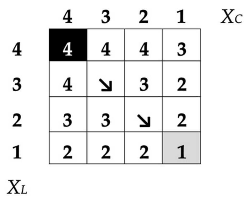
In the numerically coded risk matrix, the risk probability categories are shown along the vertical axis (variables X_L ∊ L (likelihood) and the value of hazard classes (categories) that considers the severity of consequences from the onset of risks is along the horizontal axis (X_C ∊ C (consequences). The sets of numerical values of the introduced variables are given as L = {1, 2, 3, 4} and C = {1, 2, 3, 4}. The sets L and C are the basis of the numerical risk matrix (Figure 2).

The filling of the matrix starts from the lower right corner, in which the first row and the first column are located (see Figure 1 and Figure 2). This is carried out for the convenience of correlating the numerically filled matrix and the graphical risk map, which can be built by interpolating the risk matrix.

The elements of the matrix are scores corresponding to the generalized risk categories. Risk categories are defined as generalized, since they simultaneously consider both the likelihood of a risk occurring and the severity of its consequences.

The risk level will be written as X_R, X_R ∊ R, R = {1, 2, 3, 4}.

The sets of 4 risk categories {n, m, h, and e} (see Table 1), 4 categories of risk-forming parameters {a, s, c, and d} and {u, p, l, and v} (see Table 2) and the 4-point scale corresponding to them is used only in this particular case for the study.

In general, it is possible to use other scales and number of categories. The risk matrix (see Figure 2) is a subset of the Cartesian product, X_L × X_C × X_R, which determines the mapping from the set X_L × X_C to the set X_R:

M: X_L × X_C → X_R

(1)

Accordingly, the risk matrix can be interpreted as a function of two variables, X_R = M(X_L,X_C).

Let us denote the matrix element given by row r and column c as j₃.

j₃ = m_rc, m_rc ∈ M

(2)

The element that shifted 1 line up, relative to j₃, is denoted by j₄.

J₄ = m_r+1c, m_r+1c ∈ M

(3)

The element that shifted 1 column to the left, relative to j₃, is denoted by j₅.

j₅ = m_rc+1, m_rc+1 ∈ M

(4)

We will denote j₆ as the element shifted that diagonally, relative to j₃, i.e., 1 line up and 1 column to the left.

j₆ = m_r+1c+1, m_r+1c+1 ∈ M

(5)

These notations will be used to approximate the risk matrix.

3.2. Approximate Method

To approximate the risk matrix, it is proposed to use the continuous additive–multiplicative approach to aggregation proposed in [46]:

X_R(X_L,X_C) = j₃ + γ₁(j₄ − j₃) + γ₂(j₅ − j₃) + γ₁ γ₂ (j₃ + j₆ − j₄ − j₅),

(6)

where, γ₁ is the remainder of dividing the risk-forming parameter X_L by 1, and γ₂ is the remainder of dividing the risk-forming parameter X_C by 1:

γ₁ = mod(X_L;1), γ₂ = mod(X_C;1),

(7)

j₃, j₄, j₅ and j₆ are the pivot elements of the risk matrix. The pivot elements are determined according to Equations (2)–(5), where the integer value of the risk-forming parameter X_L is taken as row r, and the integer value X_C is taken as column c:

r = ⌊X_L⌋ = dim(X_L), c = ⌊X_C⌋ = dim(X_C).

(8)

The advantage of this aggregation method is the continuity, monotonicity and piecewise smoothness of the function (6), which allows it to be used in formulating the problem of optimal risk management.

The monotonicity of function (6) can be seen from Equation (9), which is obtained by small transformations [47]:

X_R(X_L,X_C) = j₃ (1 − γ₁) (1 − γ₂) + j₄ (1 − γ₁) γ₂ + j₅ (1 − γ₂) γ₁ + j₆ γ₁ γ₂

(9)

Equation (7) shows that all terms in (9) cannot be negative, since γ1, γ2 ∈ [0; 1). Due to additivity, it is seen that Equation (9) describes a monotonically increasing function. The requirement that the risk matrix does not decrease can be explained by the fact that the risk cannot decrease as any of the risk-forming parameters increases; it will only increase with the increase in any of the risk-forming parameter. Aggregation methods based on convolution matrices are described in detail in [48].

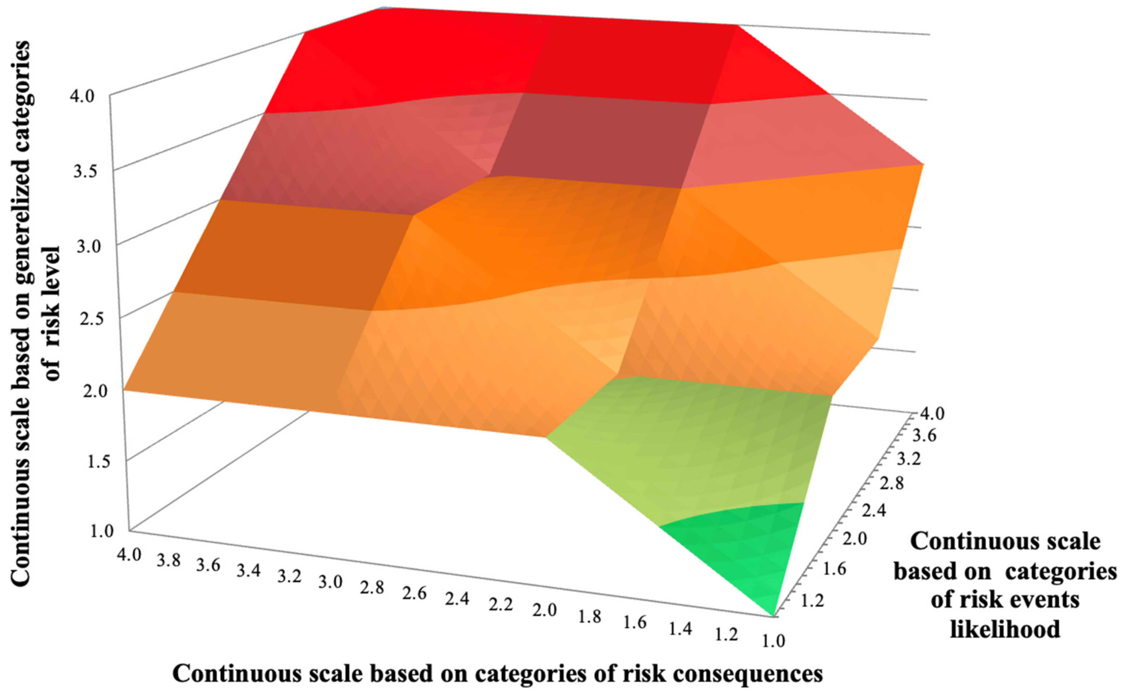
The three-dimensional risk map (Figure 3) could be built based on the risk matrix (see Figure 2). The risk matrix was interpolated using the additive–multiplicative procedure to aggregation (6)–(8) or (7)–(9).

The selected approach to aggregation (6)–(9) allows us to take into account the subjective attitude of the decision-maker to the risks in the modal judgement. This is important in case the decision-maker could not unambiguously select the risk response strategy or concrete risk category corresponding to some element of the risk matrix. In such a case, the decision-maker could form subjective attitude in a fuzzy form. It is also important in collective decision-making process, when part of the voters think it right to select one risk response strategy, while others think it right to select another response strategy.

It should be noted that, in this study, we use a 4-point scale to numerically code the risk matrix, but in general, any other scales and number of categories can be used.

3.3. Statement of the Risk Management Problem

The problem of optimal risk management is formulated under several assumptions. Let the cost functions for managing risk-forming parameters be described using quadratic equations:

C(X_L) = a_L·X_L² + b_L·X_L + c_L,

(10)

C(X_C) = a_C·X_C² + b_C·X_C + c_C.

(11)

Cost function (10) describes the dependence of costs on reducing risk event likelihood. Cost function (11) describes the dependence of costs on mitigating risk consequences.

Cost functions (10) and (11) correspond to the inverse function of a special case of the Cobb–Douglas production function.

An original Cobb–Douglas production function [49] is expressed as:

Q = A·K^α·L^β.

(12)

where, Q—total production; A—factor productivity; K—capital input (a measure of all machinery, equipment, and buildings; the value of capital input divided by the price of capital); L—labor input; and a and b—output elasticities of capital and labor, respectively (0 < a, b < 1).

A special case of the Cobb–Douglas production function (12) is expressed as (13),

X = A·C^a.

(13)

where, X is the real value of all goods resulting from the investment of costs C (symbol C performed instead of K). Expressing C from expression (13), we obtain,

C = (X/A)^1/a = a_c·X^1/a.

(14)

In a special case parameter, a could be one half, thus, cost function (14) correspond to the second-order polynomial with zero quadratic coefficients b_C and c_C. In general cases, we obtain quadratic equations like (10), and (11).

Total costs to risk management is expressed as a sum of costs on reducing risk event likelihood C(X_L) and costs on mitigating risk consequences C(X_C).

Therefore, the risk management problem is solved by minimizing the total cost of managing both the risk-forming parameters,

C(X_L) + C(X_C) → min

(15)

with constraints on risk-forming parameters falling within the range of domain values:

X_L ∈ L, X_C ∈ C,

(16)

and provided that the combination of risk-forming parameters results in a given level of risk:

X_R = M(X_L; X_C),

(17)

The problem is solved by varying the values of the risk level in the constraint (17), which will find the set that forms the risk management trajectory.

Key assumption means that the risk management problem is solved for each risk factor separately.

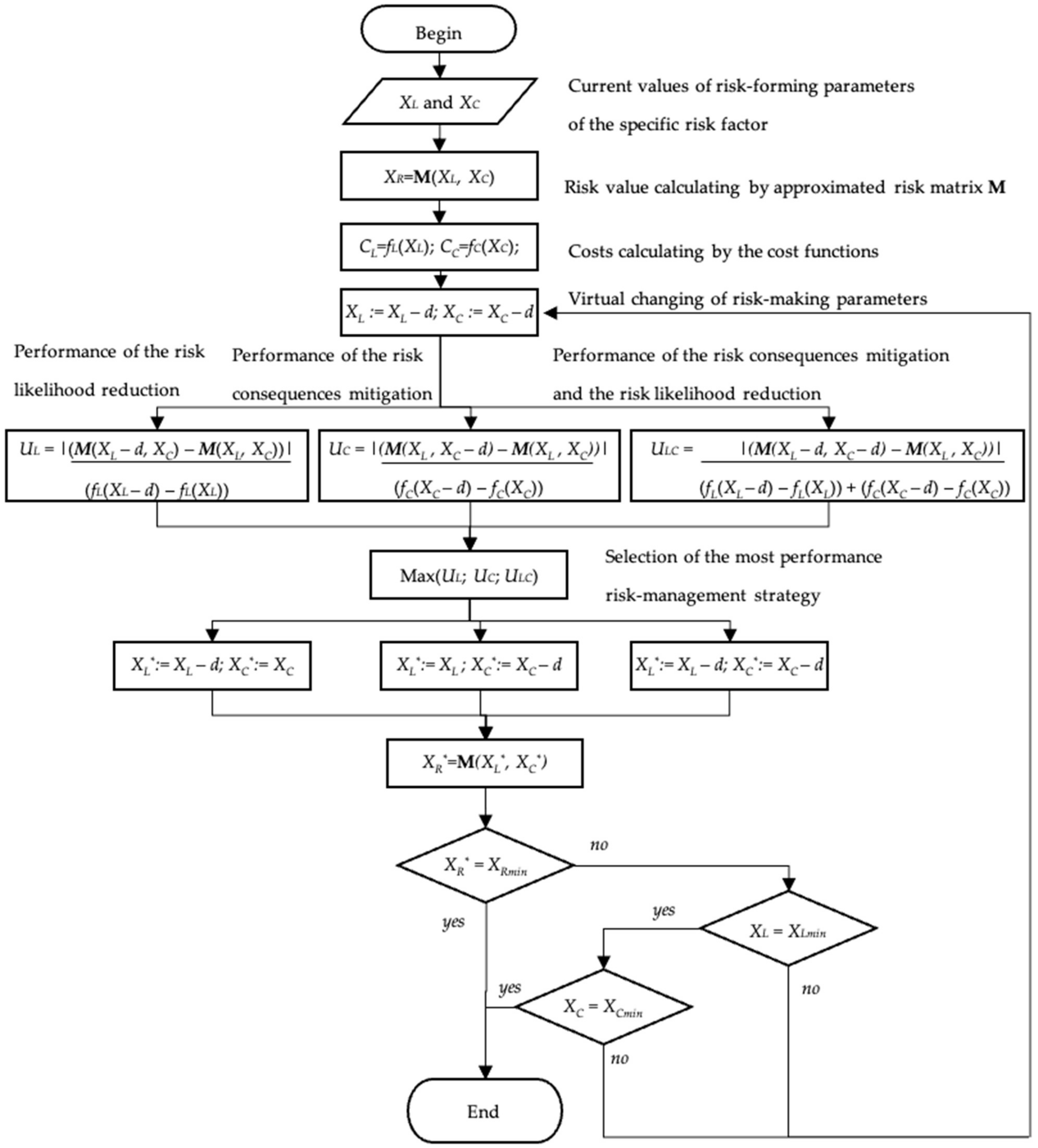
Flowchart of the applied method for solving the optimization problem is presented below (Figure 4).

3.4. Applied Programs

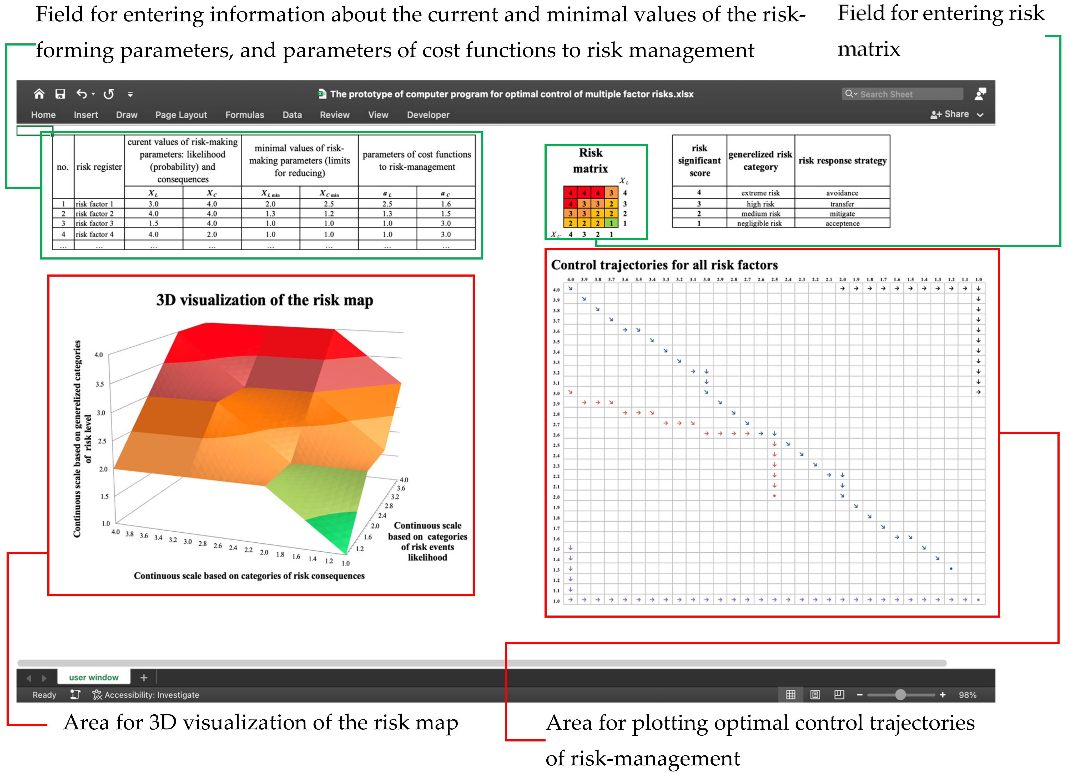
The convenience of the above methods lies in the fact that they can be used not via special software, but with the help of usual spreadsheets. In this study, a prototype of an information system for optimal management of multifactorial risks was created by using spreadsheets Microsoft^® Excel for Mac (Version 16.74 (23061100) Retail License 2019).

Figure 5 shows the screenshot of the information system prototype and fields available to change by user: for entering risk matrix correspond to the decision-maker’s subjective attitude towards risks; entering information about the current and minimal values of the risk-forming parameters, parameters of cost functions to risk management, and also areas with automatically plotted the three-dimensional risk map and optimal control trajectories of risk-management.

Microsoft^® Excel spreadsheets are a low-code framework for developing applications and prototype of the software modules. In [50], the following arguments are presented in favor of choosing Microsoft^® Excel to create a prototype of an information system:

-

prototyping is carried out in order to create a sample information system to demonstrate the principles of operation and perform preliminary tests;

-

the resulting prototype is easy to use as an element of the technical task for programmers to create an information system;

-

Microsoft Excel spreadsheets are quite common; hence, the prototype can be demonstrated on almost any computer and users do not need to take special advanced training courses; and

-

work in Microsoft Excel does not require advanced programming skills, which will allow users to modify the prototype of the information system on their own.

We also found many examples of scholarly studies, wherein spreadsheets like Excel are used for the risk assessment and risk management tasks. For example, Excel and Visual Basic for Application (VBA) are used for credit risk modeling [50].

In the books, “Credit risk modeling using Excel and VBA” [51], “Market risk analysis, practical financial econometrics” [52], and “Operational Risk with Excel and VBA: Applied Statistical Methods for Risk Management” [53] Excel and VBA are used for the demonstration of statistical methods. Monte Carlo simulation in risk management in projects using Excel is described in [54]. Many more such examples can be found in the literature.

4. Results

Table 3. Model parameter examples.

No.	Risk Register	Current Values of Risk-Forming Parameters: Likelihood (Probability) and Consequences		Minimal Values of Risk-Forming Parameters (Limits for Reducing)
		XL	XC	XLmin	XCmin
1	Risk factor 1	3.0	4.0	2.0	2.5
2	Risk factor 2	4.0	4.0	1.3	1.2

shows the current positions of the risk-forming parameters of the two conceptual risk factors, the limits of their reduction because of managing each individual risk, as well as the parameters of functions that describe the costs of risk management.

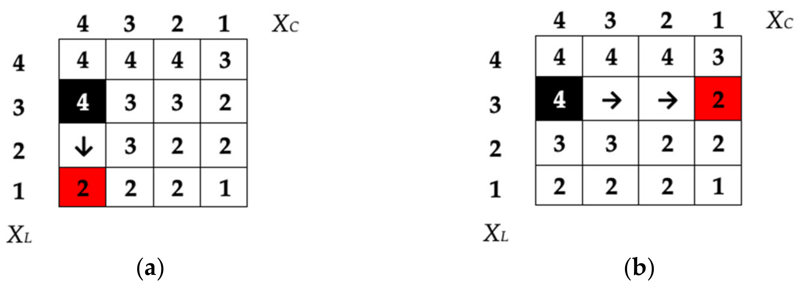
Consider all risk factors (Table 3) separately. Begin from the first risk factor no. 1. Current values of risk-forming parameters are the following: X_L = 3; and X_C = 4. Let the decision-maker has subjective attitude towards risks as was shown above (see Figure 1) and its opinion formed as the numerical coded risk matrix (see Figure 2). Element of risk matrix corresponding to the starting position is highlighted in black. The decision-maker could apply several risk-management strategies (Figure 6) and (Figure 7).

The first strategy (Figure 6a) implies reducing risk likelihood or probability, but according to the constraint on the minimal value of X_L (see Table 3, X_Lmin = 2), the goal position (X_L = 1, and X_C = 4; element highlighted in red) is not possible.

The next strategy (Figure 6b) implies mitigation of risk consequences, but according to the constraint on the minimal value of X_C (see Table 3, X_Cmin = 2.5), the goal position (X_L = 3, and X_C = 1; element highlighted in red) herein too is not possible.

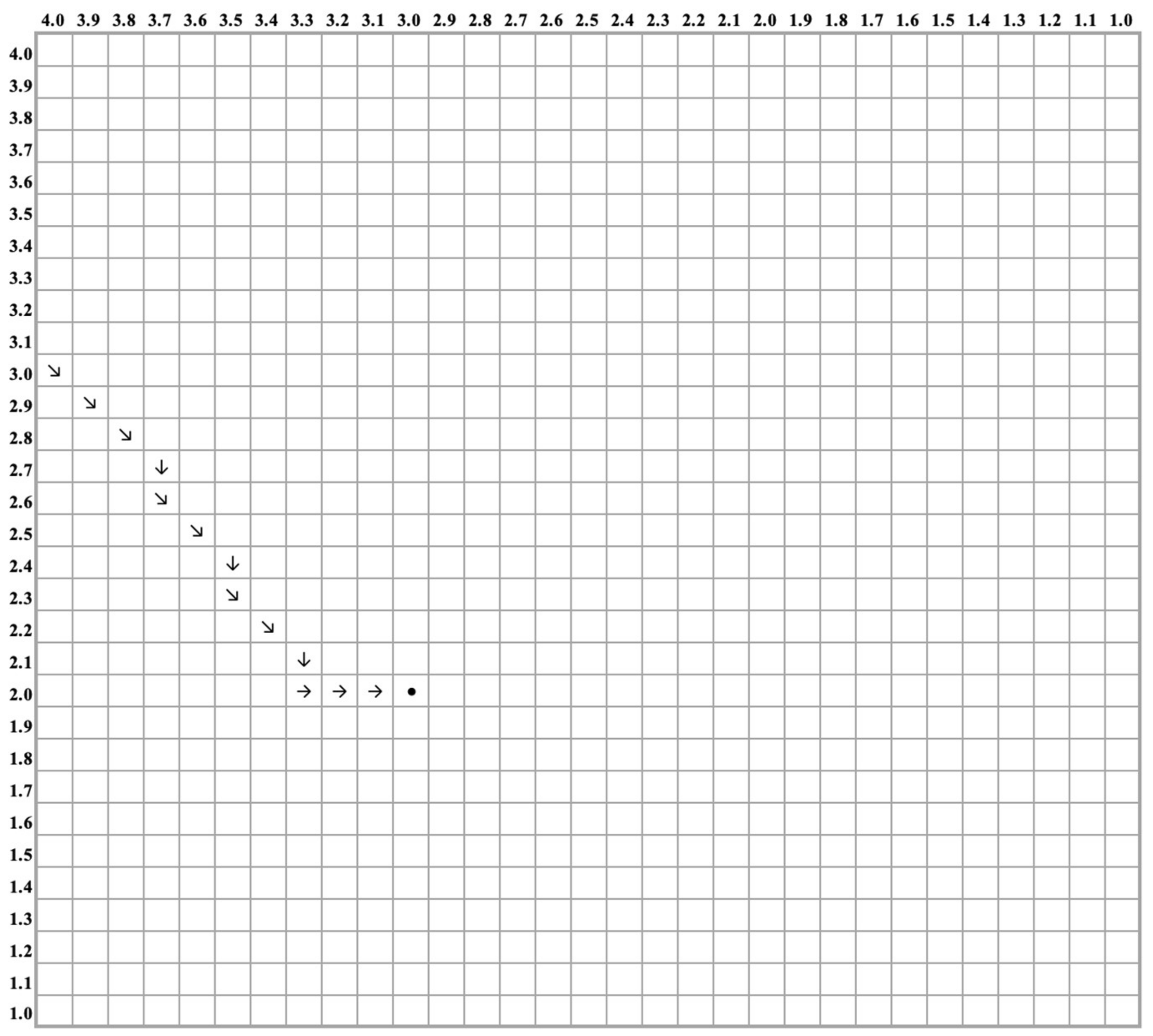
Therefore, the decision-maker should combine strategies. The first combination strategy (Figure 7a) allows to reach the minimal available value of X_Lmin = 2 and follows mitigation of risk consequences until reaching the minimal available value of X_Cmin = 2.5. Such an approach allows the decision-maker to come near to the highlighted area in grey element (X_L = 3, and X_C = 2). Because of the constraints on the minimal value of X_C, the real position of risk factor no. 1 will be X_L = 3, and X_C = 2.5. The decision-maker could obtain a similar result by mitigating risk consequences in the first stage and by additionally reducing the risk probability in the next step (Figure 7b).

Selection between these strategies (Figure 7a or Figure 7b) depends on the costs of risk-forming parameters management. If mitigation of risk consequences is cheaper than reducing risk likelihood, then the latter strategy (Figure 7b) will be better. If not, the first strategy should be selected by the decision-maker.

Consider the risk matrix with no integer values in the basis of axes and plot the control trajectory nearly to optimal.

Let the polynomial parameters of cost functions differ only by coefficients a_L and a_C.

Coefficient a_C (18) should be less than a_L (19) to provide the condition for mitigation of risk consequences being cheaper than reducing risk probability.

C(X_C) = 1.6·X_C²,

(18)

C(X_L) = 2.5·X_L².

(19)

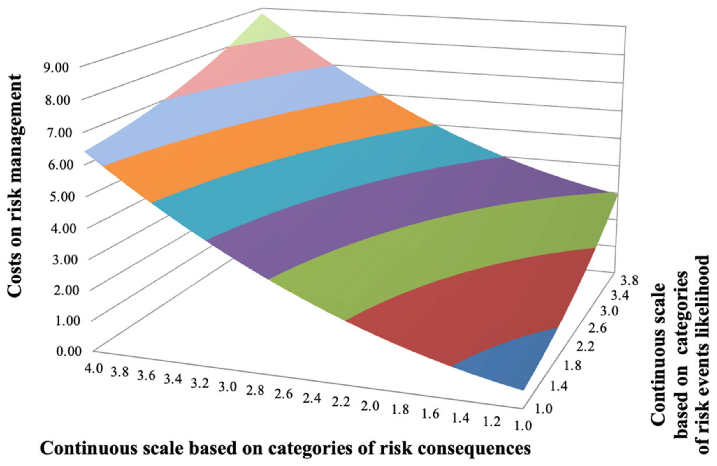
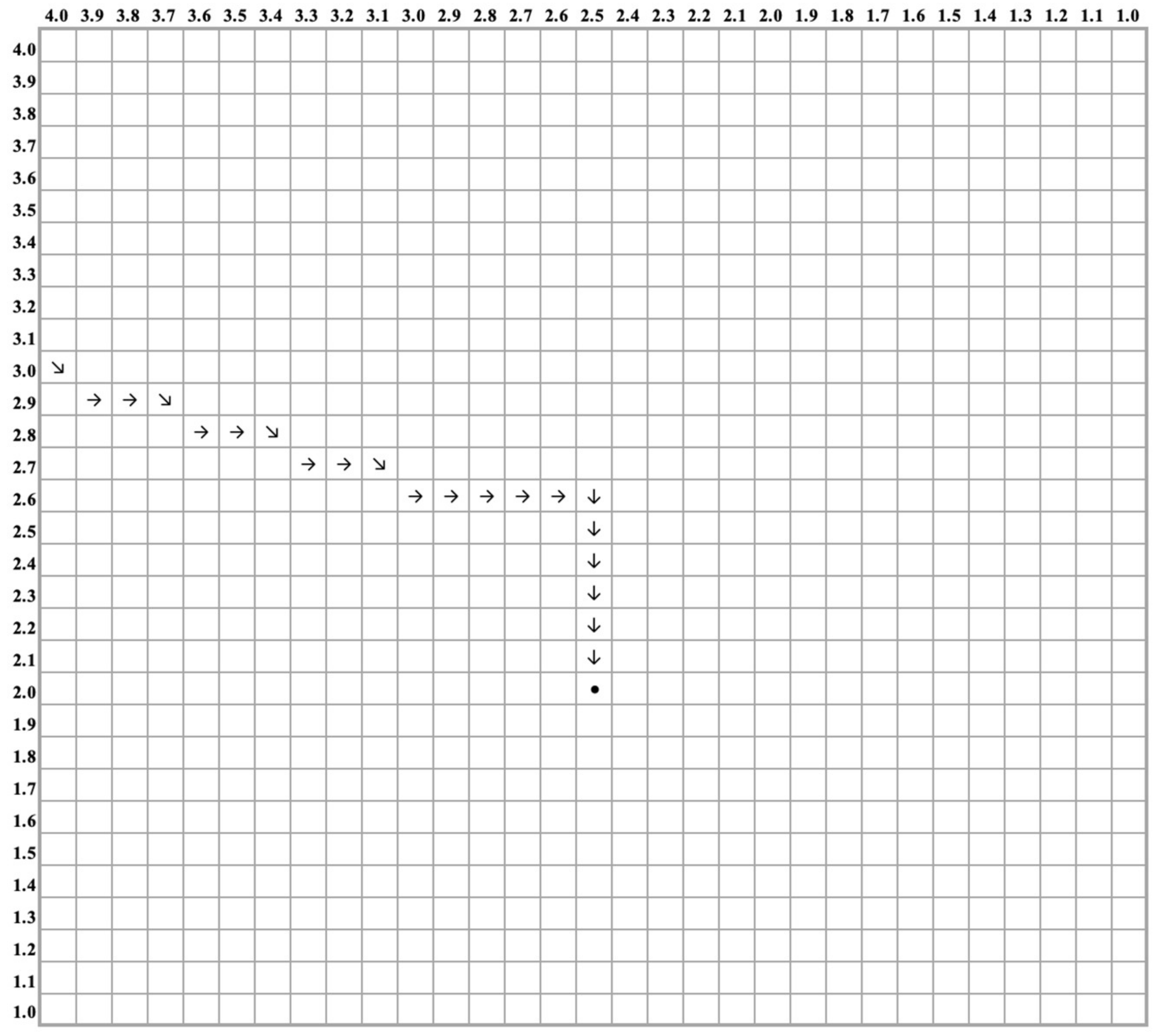
The influence of costs on risk management (Figure 8) and the optimal control trajectory (Figure 9) are shown below. Optimality implies that any local deviation from the trajectory will incur more cost. As we have already noted in the section “methods”, a numerical method (see Figure 5) is used for search of optimal risk management trajectories, based on the choice of the most effective direction. The effectiveness of directions is defined as the ratio of change in risk to change in costs.

Consider matching the second case to coefficient a_L (20) less than a_C (21):

C(X_L) = 1.6·X_L²,

(20)

C(X_C) = 2.5·X_C².

(21)

The influence of costs on risk management (Figure 10) and the optimal control trajectory (Figure 11) are shown below.

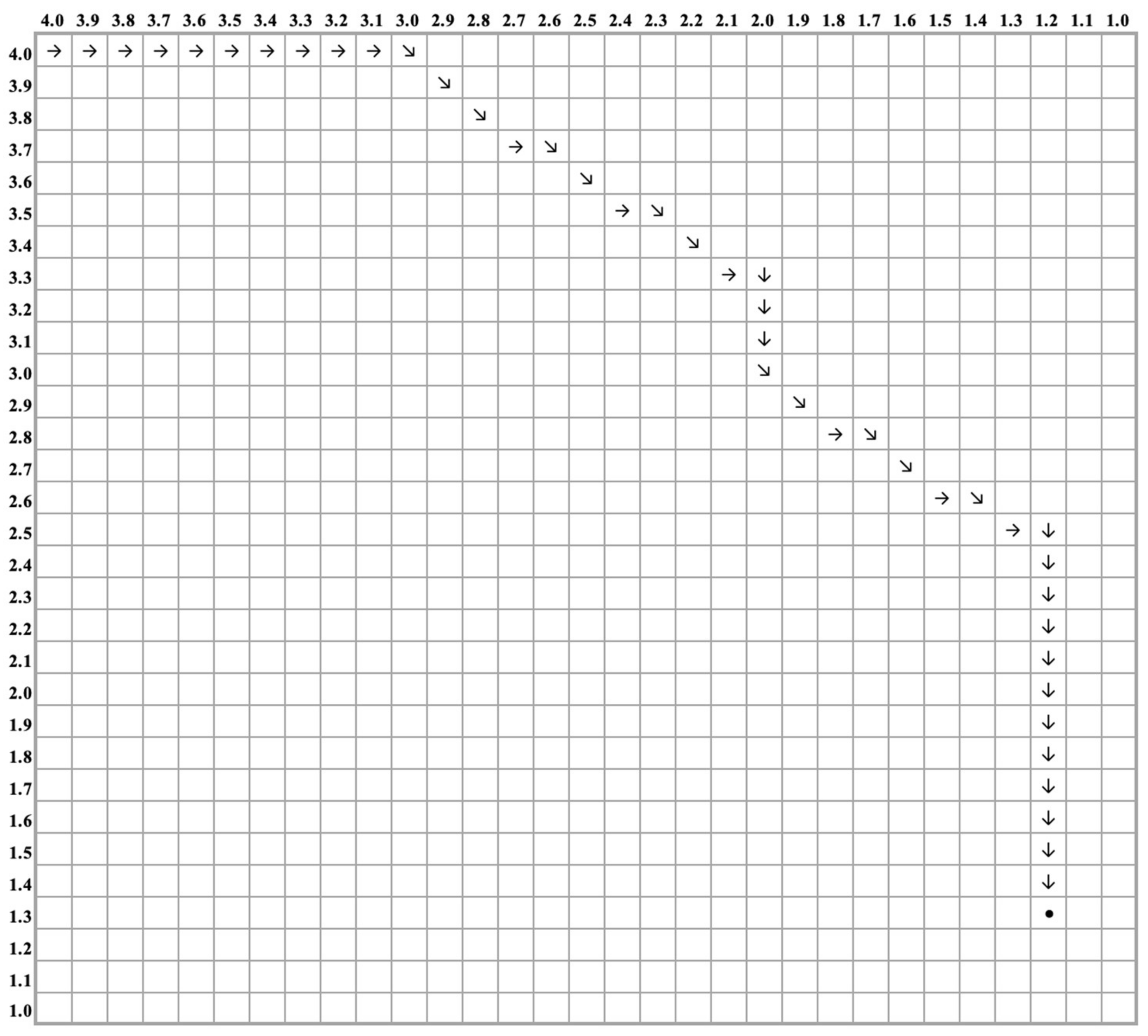
Consider the second illustrated risk factors no. 2 (see Table 3). Current values of risk-forming parameters are the following: X_L = 4, and X_C = 4. The element of risk matrix corresponding to the start position is highlighted in black again (Figure 12) as it was above (see Figure 6 or Figure 7). In this case, it is obvious that the only correct strategy is to opt for the mitigation of risk consequences and reducing risk probability together, because only on one element, it has minimal value X_Rmin = 1 (see Figure 12). This element match to X_L = 1, and X_C = 1.

However, strategy of both mitigation of risk consequences and reducing risk probability (see Figure 12) are not optimal, because the decision-maker incurs more costs. Taking into account the costs to risk management, optimal control trajectory will be following (Figure 13).

The algorithm to find the optimal risk management trajectory used in this paper is based on the principle of finding the local most effective behavior strategies, starting from the initial position, and iteratively changing the state of the object each time until the minimum is reached by the value of the complex indicator, that is, the risk level, which acts as an objective function.

Optimality is understood as the achievement of the minimum expenditure of resources to ensure the desired state. It should be noted that the found trajectory can be considered optimal under given restrictions on the possible values of the arguments (risk-forming parameters). However, without the constraints on the discrete values of the arguments, there is a more efficient control trajectory (which can be found via analytical solution (see [41]). Therefore, the trajectory found numerically should be called approximate to the optimal trajectory, or a reservation should be made on the restriction.

The most efficient strategy is sought in accordance with the solution of the knapsack problem, where it is necessary to choose alternatives that have the maximum value of the indicator calculated as the ratio of effect to costs (in this study, the ratio of risk reduction to the change in resource costs to ensure a potential state).

5. Conclusions and Discussion

This study proved hypothesis H1: the use of modern mathematical methods makes it possible to create a tool for managing multifactor risks and optimize the costs of their management.

In this study, a system prototype was created that supports the management of up to two risk factors based on the introduction of any monotonic risk matrix of 4 × 4 dimensions, which is a physical limitation for a real risk management system in enterprises. This limitation is expected to be eliminated during further development of the system.

The second direction of future research and development in this area is to expand the functionality of the system and determine the state of optimal risk management, considering the costs of borrowed funds. The introduction of the factor of external financing into the system is extremely important since interest rates on a loan also directly depend on the magnitude of risk.

Preliminary studies have shown that the limitations present in this model can be overcome with further development. Moreover, the results of this study expand the area of scientific literature devoted to mathematical methods of risk management and the development of an information system for optimal management of multifactorial risks.

References

1. Brandenburg, M.; Rebs, T. Sustainable supply chain management: A modeling perspective. Ann. Oper. Res. 2015, 229, 213–252. [Google Scholar] [CrossRef]
2. Lin, T.T.; Yen, H.-T.; Hsu, S.-Y. A Synergy Value Analysis of Sustainable Management Projects: Illustrated by the Example of the Aesthetic Medicine Industry. J. Risk Financ. Manag. 2022, 15, 348. [Google Scholar] [CrossRef]
3. Willett, A.H. The Economic Theory of Risk and Insurance; P.S. King & Son: London, UK, 1901; 142p. [Google Scholar]
4. Nosratabadi, S.; Mosavi, A.; Shamshirband, S.; Zavadskas, E.K.; Rakotonirainy, A.; Chau, K.W. Sustainable business models: A review. Sustainability 2019, 11, 1663. [Google Scholar] [CrossRef] [Green Version]
5. Haimes, Y.Y. Risk Modeling, Assessment, and Management, 2nd ed.; First published 1998; John Wiley & Sons, Inc.: Hoboken, NJ, USA, 2004; p. 837. [Google Scholar]
6. Gracheva, M.V.; Sekerin, A.B.; Afanasyev, A.M.; Babaskin, S.Y.; Bykova, A.G.; Volkov, I.M.; Kopytin, K.V.; Nikitin, S.A.; Pervushin, V.A.; Svetlov, N.M.; et al. Risk-Management of Investment Project; Unity-Dana: Moscow, Russia, 2012; p. 544. [Google Scholar]
7. Mazumder, M.; Hossain, D.M. Research on corporate risk reporting: Current trends and future avenues. J. Asian Financ. Econ. Bus. 2018, 5, 29–41. [Google Scholar] [CrossRef]
8. Yang, S.; Ishtiaq, M.; Anwar, M. Enterprise risk management practices and firm performance, the mediating role of competitive advantage and the moderating role of financial literacy. J. Risk Financ. Manag. 2018, 11, 35. [Google Scholar] [CrossRef] [Green Version]
9. Hsu, M.-F.; Hsin, Y.-S.; Shiue, F.-J. Business analytics for corporate risk management and performance improvement. Ann. Oper. Res. 2021, 315, 629–669. [Google Scholar] [CrossRef]
10. Villanueva, E.; Nuñez, M.A.; Martins, I. Impact of Risk Governance, Associated Practices and Tools on Enterprise Risk Management: Some Evidence from Colombia. Rev. Finanz. Política Económica 2022, 14, 187–206. [Google Scholar] [CrossRef]
11. Dragomir, V.D. Theoretical aspects of environmental strategy. In Corporate Environmental Strategy; Springer: Cham, Switzerland, 2020; pp. 1–31. [Google Scholar] [CrossRef]
12. Chaudhuri, A.; Boer, H.; Taran, Y. Supply chain integration, risk management and manufacturing flexibility. Int. J. Oper. Prod. Manag. 2018, 38, 690–712. [Google Scholar] [CrossRef] [Green Version]
13. Fan, Y.; Stevenson, M. A review of supply chain risk management: Definition, theory, and research agenda. Int. J. Phys. Distrib. Logist. Manag. 2018, 48, 205–230. [Google Scholar] [CrossRef] [Green Version]
14. Singh, N.P. Managing environmental uncertainty for improved firm financial performance: The moderating role of supply chain risk management practices on managerial decision making. Int. J. Logist. Res. Appl. 2020, 23, 270–290. [Google Scholar] [CrossRef]
15. El Baz, J.; Ruel, S. Can supply chain risk management practices mitigate the disruption impacts on supply chains’ resilience and robustness? Evidence from an empirical survey in a COVID-19 outbreak era. Int. J. Prod. Econ. 2021, 233, 107972. [Google Scholar] [CrossRef]
16. Elmsalmi, M.; Hachicha, W.; Aljuaid, A.M. Prioritization of the Best Sustainable Supply Chain Risk Management Practices Using a Structural Analysis Based-Approach. Sustainability 2021, 13, 4608. [Google Scholar] [CrossRef]
17. Mingaleva, Z.; Deputatova, L.; Starkov, Y. Management of Organizational Knowledge as a Basis for the Competitiveness of Enterprises in the Digital Economy. Lect. Notes Netw. Syst. 2020, 78, 203–212. [Google Scholar] [CrossRef]
18. Lee, J.; Lee, D.K. Application of industrial risk management practices to control natural hazards, facilitating risk communication. Int. J. Geo-Inf. 2018, 7, 377. [Google Scholar] [CrossRef] [Green Version]
19. Krause, T.A.; Tse, Y. Risk management and firm value: Recent theory and evidence. Int. J. Account. Inf. Manag. 2016, 24, 56–81. [Google Scholar] [CrossRef]
20. Eriandani, R.; Wijaya, L.I. Corporate Social Responsibility and Firm Risk: Controversial Versus Noncontroversial Industries. J. Asian Financ. Econ. Bus. 2021, 8, 953–965. [Google Scholar] [CrossRef]
21. Kim, S.; Lee, G.; Kang, H.-G. Risk management and corporate social responsibility. Strateg. Manag. J. 2021, 42, 202–230. [Google Scholar] [CrossRef]
22. Kuo, Y.-F.; Lin, Y.-M.; Chien, H.-F. Corporate social responsibility, enterprise risk management, and real earnings management: Evidence from managerial confidence. Financ. Res. Lett. 2021, 41, 101805. [Google Scholar] [CrossRef]
23. Renault, B.; Agumba, J.; Ansary, N. An exploratory factor analysis of risk management practices: A study among small and medium contractors in Gauteng. Acta Structilia 2018, 25, 1–39. [Google Scholar] [CrossRef] [Green Version]
24. Joshi, H. Corporate risk management, firms’ characteristics and capital structure: Evidence from Bombay Stock Exchange (BSE) Sensex Companies. Vision 2018, 22, 395–404. [Google Scholar] [CrossRef]
25. Busru, S.A.; Shanmugasundaram, G.; Bhat, S.A. Corporate governance an imperative for stakeholders protection: Evidence from risk management of Indian listed firms. Bus. Perspect. Res. 2020, 8, 89–116. [Google Scholar] [CrossRef]
26. Girangwa, K.G.; Rono, L.; Mose, J. The influence of enterprise risk management practices on organizational performance: Evidence from Kenyan State Corporations. J. Account. Bus. Financ. Res. 2020, 8, 11–20. [Google Scholar] [CrossRef] [Green Version]
27. Avdiysky, V.I.; Bezdenezhnykh, V.M.; Katayeva, E.G. Risk management as a key element of ensuring the implementation of the risk-oriented approach in the activities of business entities. Econ. Taxes Right 2017, 10, 6–15. [Google Scholar]
28. Akatov, N.; Mingaleva, Z.; Klačková, I.; Galieva, G.; Shaidurova, N. Expert Technology for Risk Management in the Implementation of QRM in a High-Tech Industrial Enterprise. Manag. Syst. Prod. Eng. 2019, 27, 250–254. [Google Scholar] [CrossRef] [Green Version]
29. DuHadway, S.; Carnovale, S.; Hazen, B. Understanding risk management for intentional supply chain disruptions: Risk detection, risk mitigation, and risk recovery. Ann. Oper. Res. 2019, 283, 179–198. [Google Scholar] [CrossRef]
30. Vincent, N.E.; Higgs, J.L.; Pinsker, R.E. Board and management-level factors affecting the maturity of IT risk management practices. J. Inf. Syst. 2019, 33, 117–135. [Google Scholar] [CrossRef]
31. Liu, B.; Niu, Y.; Zhang, Y. Corporate liquidity and risk management with time-inconsistent preferences. Econ. Model. 2019, 81, 295–307. [Google Scholar] [CrossRef]
32. Hao, J.P.; Kang, F. Corporate environmental responsibilities and executive compensation: A risk management perspective. Bus. Soc. Rev. 2019, 124, 145–179. [Google Scholar] [CrossRef] [Green Version]
33. Tai, V.W.; Lai, Y.-H.; Yang, T.-H. The role of the board and the audit committee in corporate risk management. N. Am. J. Econ. Financ. 2020, 54, 100879. [Google Scholar] [CrossRef]
34. Cassano, R. Corporate global responsibility and reputation risk management. Symphonya Emerg. Issues Manag. 2019, 1, 129–142. [Google Scholar] [CrossRef] [Green Version]
35. Catanzaro, A.; Teyssier, C. Export promotion programs, export capabilities, and risk management practices of internationalized SMEs. Small Bus. Econ. 2021, 57, 1479–1503. [Google Scholar] [CrossRef]
36. Christopher, J.; Sarens, G. Diffusion of Corporate Risk-Management Characteristics: Perspectives of Chief Audit Executives through a Survey Approach. Aust. J. Public Adm. 2018, 77, 427–441. [Google Scholar] [CrossRef]
37. Wahlström, B. Models, modelling and modellers: An application to risk analysis. Eur. J. Oper. Res. 1994, 75, 477–487. [Google Scholar] [CrossRef]
38. Alekseev, A. Stability analysis of the rating and control mechanism to agent’s strategic behavior (on example of the risk management policy coordination). Appl. Math. Control Sci. 2019, 4, 136–154. [Google Scholar] [CrossRef]
39. Mingaleva, Z.A.; Lobova, E.S. “Portfolio analysis of innovative projects, taking into account endogenous and exogenous risks”. Programmy Dlia EVM. Bazy Dannykh. Topologii Integral’nykh Mikroskhem [Computer Programs. Database. Topologies of Integrated Circuits]. Computer program RU 2022664434. 29 July 2022. [Google Scholar]
40. Jiang, J.; Feng, Y. The interaction of risk management tools: Financial hedging, corporate diversification and liquidity. Int. J. Financ. Econ. 2021, 26, 2396–2413. [Google Scholar] [CrossRef]
41. Alekseev, A. Control of a complex objects, states of which are describing by the matrix rating mechanisms. Appl. Math. Control Sci. 2020, 1, 114–139. [Google Scholar] [CrossRef] [PubMed]
42. Mingaleva, Z.; Akatov, N.; Butakova, M. A Syndinic approach to enterprise risk management. Lect. Notes Netw. Syst. 2021, 315, 293–305. [Google Scholar] [CrossRef]
43. Beyth-Marom, R. How probable is probable? A numerical translation of verbal probability expressions. J. Forecast. 1982, 1, 257–269. [Google Scholar] [CrossRef]
44. Ristić, D. A tool for risk assessment. Saf. Eng. 2013, 3, 121–127. [Google Scholar] [CrossRef]
45. Thomas, P.; Bratvold, R.B.; Bickel, J.E. The risk of using risk matrices. SPE Econ. Manag. 2014, 6, 56–66. [Google Scholar] [CrossRef]
46. Alekseev, A. The additive-multiplicative fuzzy aggregation matrix mechanism and equivalent it’s the continuous mechanism. In Proceedings of the 12th International Scientific and Practical Conference “Modern Complex Control Systems 2017”, Lipetsk, Russia, 25–27 October 2017; Volume 1, pp. 15–20. [Google Scholar]
47. Alekseev, A. On strategy-proofness of matrix integrated rating mechanism. In Proceedings of the Socio-Physics and Socio-Engineering, Moscow, Russia, 23–25 May 2018; pp. 179–180. [Google Scholar]
48. Alekseev, A.; Salamatina, A.; Kataeva, T. Rating and Control Mechanisms Design in the Program “Research of Dynamic Systems”. In Proceedings of the 2019 IEEE 21st Conference on Business Informatics (CBI), Moscow, Russia, 15–17 July 2019; pp. 96–105. [Google Scholar] [CrossRef]
49. Cobb, C.W.; Douglas, P.H. A Theory of production. Am. Econ. Rev. 1928, 18, 139–165. [Google Scholar]
50. Alekseev, A.; Noskova, A.; Neifeld, V. The Software Modules “Insider” as a KYC-Solution for Industrial Verification and Bankruptcy Prediction. In Proceedings of the 2022 4th International Conference on Control Systems, Mathematical Modeling, Automation and Energy Efficiency (SUMMA), Lipetsk, Russia, 9–11 November 2022; pp. 623–626. [Google Scholar] [CrossRef]
51. Löffler, G.; Posch, P.N. Credit Risk Modeling Using Excel and VBA; John Wiley & Sons Ltd.: Hoboken, NJ, USA, 2007; p. 278. [Google Scholar]
52. Alexander, C. Market Risk Analysis, Practical Financial Econometrics; John Wiley & Sons Ltd.: Chichester, UK, 2008; p. 387. [Google Scholar]
53. Lewis, N. Operational Risk with Excel and VBA: Applied Statistical Methods for Risk Management; John Wiley & Sons, Inc.: Hoboken, NJ, USA, 2004; 259p. [Google Scholar]
54. Tysiak, W.; Sereseanu, A. Monte Carlo simulation in risk management in projects using Excel. In Proceedings of the IEEE International Workshop on Intelligent Data Acquisition and Advanced Computing Systems: Technology and Applications, Cosenza, Italy, 21–23 September 2009; pp. 581–585. [Google Scholar]
Figure 1. An example of risk response strategies formed in a risk matrix for a decision-maker, taking into account his subjective attitude to risk-forming parameters. In this figure fill colors correspond to risk response strategies: red—avoidance; orange—transfer; yellow—mitigate; and green—acceptance.
Computation 11 00132 g001
Figure 2. An example of a numerically coded risk matrix. In this figure fill colors correspond to the risk significant scores; the last ones correspond to the risk levels: red—4 (extremal risk); orange—3 (high risk); yellow—2 (medium risk); and green—1 (negligible risk).
Computation 11 00132 g002
Figure 3. The surface of a continuous convolution function of risk-forming parameters obtained by interpolation of the risk matrix. In this figure fill colors correspond to the following intervals of risk level values: bright green corresponds to the interval from 1.0 up 1.5; pale green corresponds to the interval 1.5–2.0; yellow corresponds to the interval 2.0–2.5; orange correspond to the interval 2.5–3.0; pale red to the range 3.0–3.5; and bright red corresponds to the interval 3.5–4.0.
Computation 11 00132 g003
Figure 4. Flowchart of the numerical method for solving the optimization problem. Sign * means the most performance risk-management strategy, selected between UL, UC and ULC.
Computation 11 00132 g004
Figure 5. Screenshot of the prototype information system for optimal management of multifactorial risks created in Microsoft® Excel for Mac. Green rectangles correspond to the fields available to change by user; red rectangles correspond to the areas with automatically plotted the three-dimensional risk map and optimal control trajectories of risk-management.
Computation 11 00132 g005
Figure 6. The individual strategies of the risk factor no. 1 management (initial values, XL = 3; XC = 4) available to the decision-maker: (a) strategy of reducing risk likelihood; (b) strategy of mitigation of risk consequences. Element of risk matrix corresponding to the starting position is highlighted in black. The goal elements highlighted in red, because are not possible according to the constraint on the minimal value of XL and XC.
Computation 11 00132 g006
Figure 7. The combined strategies of the risk factor no. 1 management (initial values, XL = 3; XC = 4) available to the decision-maker: (a) combined strategy of reducing risk likelihood to condition and following mitigation of risk consequences; (b) combined strategy of risk consequences mitigation at the first stage and following reducing risk likelihood measures together with mitigation of risk consequences. Starting position is highlighted in black as was above, goal element is highlighted in grey, but it is near to the available to the decision-maker finish position (XL = 3, and XC = 2.5).
Computation 11 00132 g007
Figure 8. The surfaces of total costs on risk management in case of cost functions (18) and (19).
Computation 11 00132 g008
Figure 9. Approximation of optimal control trajectory of risk factor no. 1 in case of cost functions (18) and (19).
Computation 11 00132 g009
Figure 10. The surfaces of total costs on risk management in case of cost functions (20) and (21).
Computation 11 00132 g010
Figure 11. Approximation of optimal control trajectories of risk factor no. 1 with in case of cost functions (20) and (21).
Computation 11 00132 g011
Figure 12. The second risk factor no. 2 management (initial values, XL = 4; XC = 4) direction the global strategy available to the decision-maker. Starting position is highlighted in black as was above, goal element is highlighted in grey.
Computation 11 00132 g012
Figure 13. Approximate to optimal control trajectories of risk factor no. 2 (initial values, XL = 4; XC = 4) in case of cost functions (20) and (21).
Computation 11 00132 g013